ACTIVE CONTROL OF CENTRIFUGAL COMPRESSOR SURGE
by
Judith Ellen Pinsley B.S., Cornell University (1986)
SUBMITTED IN PARTIAL FULFILLMENT OF THE REQUIREMENTS FOR THE
DEGREE OF
MASTER OF SCIENCE IN AERONAUTICS AND ASTRONAUTICS
at the
MASSACHUSETTS INSTITUTE OF TECHNOLOGY October 28, 1988
© Massachusetts Institute of Technology 1988
Signature of Author ý
-// ecs and Astronautics
October 28, 1988
Certified by
Prof. Edward M. Greitzer Thesis Supervisor Accepted by
'rof. H.Y. Wachman 3raduate Committee
Cas- '·
T"CCyI
LIBRARMSITHDRhkWN
ACTIVE CONTROL OF CENTRIFUGAL COMPRESSOR SURGE
by
Judith Ellen Pinsley
Submitted to the Department of Aeronautics and Astronautics on October 28, 1988 in partial fulfillment of the requirements for the Degree of Master of Science in
Aeronautics and Astronautics.
ABSTRACT
A new method for actively suppressing compressor surge in a centrifugal
compressor has been investigated through experiments supported by theory. The controller is a real-time feedback of the plenum pressure rise perturbations to a servo-actuated plenum exit throttle. Small perturbations of this control valve provide increased damping of incipient oscillations and this allows the compressor to operate stably past the normal surge line.
The controller used was based on a simple proportional control law. The theory predicts that the effectiveness of this controller is a strong function of the stability parameter B = (U/2a) Vp/(LcAin), with lower values of B leading to a higher degree of stability. The theory also determined the proportionality constant (gain) of the controller. For maximum increase in stable flow range, a controller phase of zero degrees was found to hold for all operating conditions with the gain set within limits determined by the system parameters. The model predicts, and the experiments confirm, that with control the compression system resonant frequency and perturbation growth rate are changed.
Based upon the success of preliminary low speed tests, a high speed facility was constructed for operating a small turbocharger at realistic pressure ratios. The experimental results showed that active throttle control is a viable means to suppress surge and operate within a previous inaccessible region. A reduction of 25% in the surge point mass flow was achieved over a range of operating
conditions. Surge line extension was found to be strongly B dependent. Time-resolved measurements showed that suppression of surge oscillations was achieved with relatively little power input to the control valve. The throttle controller was also able to eliminate existing large amplitude surge oscillations even though the surge phenomenon is nonlinear. Comparison of experimental measurements with theoretical predictions showed that the simple model used gives adequate representation of the behavior of the compression system with a throttle controller.
Thesis Supervisor: Dr. Edward M. Greitzer
Title: Professor of Aeronautics and Astronautics
ACKNOWLEDGEMENTS
There are numerous people whom I wish to thank for their contribution to this project:
Professor Edward M. Greitzer for guidance, encouragement, and confidence in this "Smart Engines" concept.
Professor Alan H. Epstein for his practical advice on all matters of the experimental investigation.
Dr. Gerald Guenette for the long hours that he devoted to the intricacies of instrumentation and the fine points of the analysis. Thanks also for sharing the secrets of vacationing in Maine.
Holly Rathbun for her talent in handling the finances and enduring my continual questions.
Robert Haimes and David Dvore for taming the MicroVax "beast", while providing many entertaining moments along the way.
Viktor Dubrowski for his expert craftsmanship in the machine shop and his political observations.
Jim Nash and Roy Andrew for patiently teaching me all manner of laboratory procedures and helping construct the test rig.
Karen Hemmick, Nancy Martin, and Diana Park for their help on all the details.
Maj. John Craig Seymour, who preceded me to the degree list, for his keen sense of humor and for refraining from excessive conversation during the morning newspaper ritual. Also thanks to his wife Sherri and daughter Stephanie for wonderful visits to their home.
Petros Kotidis for sharing inside information on everything from file backups to Campus House of Pizza.
Gwo-Tung Chen and David Fink for the extensive groundwork they provided in the analytical and experimental world, respectively.
George Haldeman for building the first test rig and the design of the control valve.
Jim Paduano and John Simon for their perspectives from the control world and for the motor controller.
My parents, Edward and Jane Pinsley, for their love and support
throughout my life. Special thanks to my father for having an excitement about science which happily rubbed off on me.
Finally, enormous thanks to my husband-to-be, Mark Reich, for his inestimable contribution. Without his pep talks, well-placed criticism, and love this thesis would never have been possible.
The project was conducted under grants from the Army Aeropropulsion Laboratory and the Air Force Research in Aero Propulsion Technology (AFRAPT) program, and the author gratefully acknowledges this support. The author also
acknowledges the support of Mr. Harold Weber from Cummins Engine Company.
TABLE OF CONTENTS Page Abstract Acknowledgements Table of Contents List of Figures Nomenclature
Chapter 1. Introduction and Background
1.1 Introduction
1.2 Overall Approach to Surge Control
1.2.1 Previous Approaches to Surge Control 1.2.2 Active Surge Control
1.3 Scope of Present Active Control Experiment
Chapter 2. Active Throttle Control Modelling 2.1 Introduction
2.2 Model of the Compression System 2.3 System Stability Analysis
2.3.1 Positioning of System Poles
2.3.2 Stability Boundary in the Gain-Phase Plane 2.3.3 Effect of Compressor Characteristic Slope
2.3.4 Variation of Damping and Natural Frequency with Controller Phase
2.4 Summary of Control Modelling
Chapter 3. 3.1 3.2 3.3 Chapter 4. 4.1
Preliminary Results Using the Low Speed Test Facility Low Speed Test Rig
Low Speed Test Results Conclusions
High Speed Test Facility and Experimental Methods Introduction
4.2 General Facility Description 42 4.3 Turbocharger and Connecting Systems 44
4.3.1 Turbocharger Description 44
4.3.2 Inlet Duct and Instrumentation 45 4.3.2.1 Short Inlet Duct (Large B Configuration) 45 4.3.2.2 Long Inlet Duct (Small B Configuration) 47 4.3.3 Exit Duct and Instrumentation 48
4.3.4 Oiling System 49
4.4 Plenum Description and Instrumentation 50
4.4.1 Main Plenum 50
4.4.2 Secondary Plenum 51
4.4.3 Plenum Pressure Transducer Frequency Response 53
4.5 Control Valve 53
4.5.1 Valve Description 53
4.5.2 Controller Actuation 56
4.5.2.1 Control Loop Components 56
4.5.2.2 Controller Dynamics 59
4.6 Data Acquisition 61
Chapter 5. Experimental Data and Analyses 64
5.1 Introduction 64
5.2 Steady-State (Time-Averaged) Measurements 66
5.2.1 Motivation and Procedures 66
5.2.2 Uncontrolled Steady-State Compressor Performance 66 5.2.3 Controlled Steady-State Compressor Performance 70 5.2.4 B Parameter Dependence of Controllability 71 5.2.5 Summary of Steady-State Uncontrolled and Controlled 73
Measurements
5.3 Time-Resolved Measurements 74
5.3.1 Motivation and Procedures 74
5.3.2 Unsteady Behavior of the System Without Control 74
5.3.3 Unsteady Behavior of the System With Control 76
5.3.4 B Parameter Dependence of the Unsteady System Behavior 78 5.3.5 Summary of Time-Resolved Measurements 80 5.4 Comparison of Experimental Measurements to Model Predictions 81 5.4.1 Compressor Transfer Function 82
Control Action Required for Surge Line Extension Measured Stability Boundary
Shift in Measured System Resonant Frequency Conclusions
Discussion of Conclusions from This Experiment Suggestions for Further Study
References Figures Appendix A. Appendix B. Appendix C. Appendix D.
Derivation of the System Characteristic Equation Circuit Diagrams for Controller Components Derivation of Compressor Duct Effective Length
Uncertainty Analysis for Instantaneous Mass Flow
5.4.2 5.4.3 5.4.4 Chapter 6. 6.1 6.2 169 177 181 190 I
LIST OF FIGURES
1.1 Active Surge Control
1.2 Lumped Parameter Model of a Simple Compression System
1.3 Stability Criteria on the Compressor Characteristic 1.4 Surge Limit Cycle
1.5 Lumped Parameter Model of Actively Controlled Compression System
1.6 Active Volume Control Experimental Results (Huang) [9]
2.1 Model of Compression System with Plenum Exit Throttle Control
2.2 Minimum Controllable Flow Coefficient vs. Controller Phase (Chen) [1]
2.3 Root Locus for Controller at Zero Degrees Phase Shift 2.4 Minimum Controllable Flow Coefficient vs. B Parameter
2.5 Stability Boundary in the Gain-Phase Plane
2.6 Variation of Stability Boundary with B Parameter
2.7 Stability Boundary at Nominally Stable Operating Point
2.8 Effect of Compressor Characteristic Slope on System Poles
2.9 Slope Sensitivity Analysis for = .12, y Varying From 1.74 to 1.93 2.10 Slope Sensitivity Analysis for y = 1.87, 0 Varying From .08 to .14
2.11 Maximum Tolerable Compressor Characteristic Slope vs. B Parameter
2.12 Required Controller Gain for Maximum Tolerable Compressor Characteristic Slope vs. B Parameter
2.13 Variation of Perturbation Growth Rate with Controller Phase 2.14 Variation of System Resonant Frequency with Controller Phase
3.1 Low Speed Test Rig Schematic with Analog Control Loop
3.2 Holset HID Turbocharger Compressor Map
3.3 Surge Line Extension at Low Speed with Control
4.1 Flowpath for High Speed Test Facility
4.2 External Dimensions of Holset HID Turbocharger, Page 1 of 2 4.3 External Dimensions of Holset H1D Turbocharger, Page 2 of 2 4.4 Exploded View of Holset H1D Turbocharger
4.5 Typical Low Range Druck Pressure Transducer Calibration 4.6 Radial Total Temperature Profile in Compressor Exit Duct 4.7 Cross-Sectional View of Main Plenum with Volume Adjustor 4.8 Typical High Range Druck Pressure Transducer Calibration
4.9 Error in Measurement of Flowrate in Pulsating Flow vs. Hodgson Number [12] 4.10(a) Orifice Discharge Coefficient Calibration, Experimental cd vs. Reynolds
Number
4.10(b) Orifice Discharge Coefficient Calibration, Predicted cd vs. Reynolds Number [12]
4.11 Exploded View of Rotary Actuated Control Valve
4.12 Control Valve Pressure Drop vs. Mass Flow Calibration
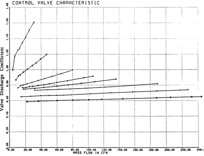
4.13(a) Measured Valve Discharge Coefficients Based on Indicated Throughflow Area
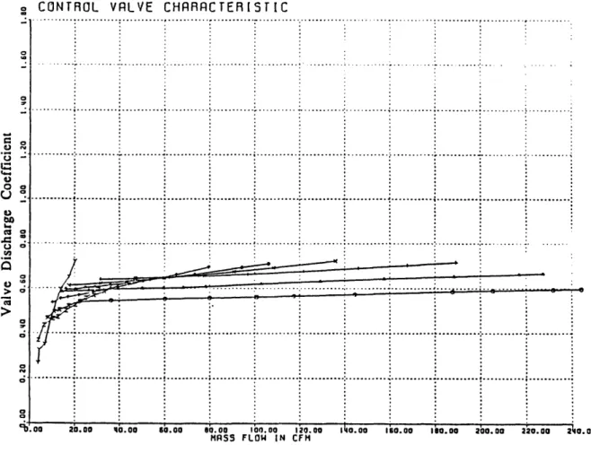
4.13(b) Measured Valve Discharge Coefficients Based on Throughflow Area with Leakage Path
4.14 Experimental "Total" Discharge Coefficient vs. Indicated Throttle Area 4.15 Motor Position Control Loop Schematic [13]
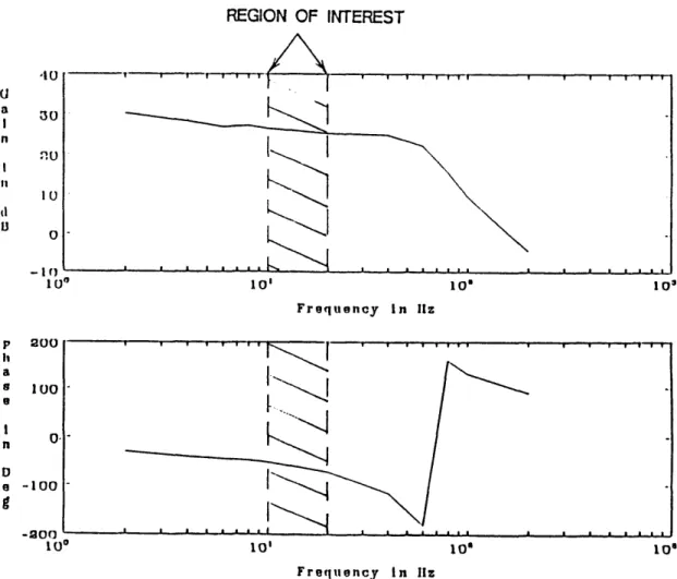
4.16 Phase Shifter and Pre-Amplifier Transfer Functions
4.17(a) Motor Position Control Loop Transfer Function, Low Level Signal
4.17(b) Motor Position Control Loop Transfer Function, High Level Signal 4.18 Overall Control Loop Transfer Function, from Phase Shifter to RVDT
4.19(a) Overall Control Loop Transfer Function Including Pressure Transducer,
Test Setup Schematic
4.19(b) Overall Control Loop Transfer Function Including Pressure Transducer, Measured Magnitude
4.19(c) Overall Control Loop Transfer Function Including Pressure Transducer, Measured Phase
4.20 Schematic of Data Acquisition Inputs and Outputs to the Controller
5.1(a) Measured Compressor Map in Small B Configuration, Pressure Ratio vs. SCFM
5.1(b) Measured Compressor Map in Small B Configuration, Psi vs. Phi 5.1(c) Measured Compressor Map in Small B Configuration, Head Coefficient
vs. Phi
5.2 Surge Line Shift with Controller, Small B Configuration
5.3 Control Effect at 90,000 RPM on Nondimensional Pressure Rise vs. Mass Flow 5.4 Compressor Adiabatic Efficiency Under Control at 90,000 RPM
5.5 Measured Compressor Map in Large B Configuration Showing Control Range
5.6 Control Effect at the Same B Parameter, Different Speed
5.7(a) Nondimensional Compressor Characteristic at 90,000 RPM Showing Measured Points
5.7(b) Nondimensional Perturbations at 90,000 RPM
5.8 Uncontrolled Mild Surge Cycles
5.9 Uncontrolled Deep Surge Cycles
5.10(a) Nondimensional Compressor Characteristic at 90,000 RPM Showing Measured Control Points
5.10(b) Nondimensional Perturbations at 90,000 RPM Under Control
5.11 Power Spectral Density of Valve Motion Under Control at Point A'
5.12 Controlled Nondimensional Pressure Rise and Mass Flow Perturbations
5.13 Nondimensional Valve Area, Plenum Pressure, and Mass Flow Perturbations
with Control in Deep Surge 5.14 Deep Surge Cycles with Control
5.16(a) Nondimensional Perturbations in Valve Area, Plenum Pressure, and Mass Flow During Controller Off-On Transient
5.16(b) Instability Cycles During Controller Off-On Transient
5.17 Nondimensional Perturbations in Valve Area, Plenum Pressure, and Mass Flow During Controller On-Off Transient
5.18 B Dependence of Surge Initiation
5.19 B Dependence of Controller Instability Frequency
5.20 Measured Compressor Transfer Function
5.21(a) Measured Compressor Map in Close-Coupled Configuration, Pressure Ratio vs. SCFM
5.21(b) Measured Compressor Map in Close-Coupled Configuration, Psi vs. Phi 5.21(c) Measured Compressor Map in Close-Coupled Configuration, Head
Coefficient vs. Phi
5.22 Comparison of Measured Controller Gain to Predicted Gain
5.23 Comparison of Measured Stability Boundary to Predicted Stability Boundary 5.24 Comparison of Measured Resonant Frequency Variation with Controller
Phase to Predicted Variation.
B.1 Phase Shifter Circuit Diagram [8] B.2 Pre-Amplifier Circuit Diagram [13]
B.3 Motor Controller Circuit Diagram [13]
B.4 Amplifier Circuit Functional Diagram, Servodynamics Corporation
C. 1 Compressor Scroll Geometry [22]
D. 1 Comparison of Surge Cycles with Actual Smoothed Data and Sine Fit Deep Surge
D.2 Comparison of Surge Cycles with Actual Smoothed Data and Sine Fit Mild Surge
NOMENCLATURE
Symbols
a -- speed of sound
-- coefficients of cubic compressor characteristic
-- coefficient of system characteristic equation
A -- cross-sectional area
-- system matrix
Aexit -- cross-sectional area of compressor exit duct
Ain -- annular impeller inlet area
A open -- wide open control valve area
AT -- throttle area
A, -- control valve area
b -- coefficient of parabolic valve characteristic
-- coefficient of system characteristic equation
b' -- "total" discharge coefficient: pressure drop in psid/(flow rate in SCFM)2
B -- stability parameter
c -- coefficient of system characteristic equation
cd -- discharge coefficient
C -- slope of valve pressure drop vs. mean valve area
Cx -- axial velocity
f -- frequency
H -- Hodgson number
L -- characteristic length
Lc -- effective compressor duct length
m -- mass flow
M -- Mach number
Nmech-- mechanical rotational speed
P -- pressure R -- radius
-- gas constant
Rex -- flat plate Reynolds number based on distance from leading edge s -- roots of system characteristic equation
t -- time
T -- slope of pressure rise (or drop) vs. mean mass flow
-- temperature U -- rotor tip speed
Vc -- compressor volume: AinLc
Vp -- plenum volume
x -- distance from leading edge in flat plate theory
zA -- complex constant for throttle control
z -- complex constant for volume control
a -- ratio of valve area to wide open valve area
f3
-- perturbation growth ratey -- specific heat ratio
8d -- boundary layer displacement thickness from flat plate theory
11 -- adiabatic compressor efficiency -- nondimensional plenum volume
-- compressor total-to-static pressure ratio p -- density
-- total temperature ratio -- nondimensional mass flow
N -- nondimensional pressure rise
x'h -- isentropic head rise coefficient w -- Helmholtz frequency of -- forcing frequency On -- natural frequency Subscripts c -- compressor
ref -- reference conditions, sea-level
t -- total
v -- control valve
0 -- ambient
-- control at zero gain -- plenum -- exit Operators 8( ) A( ) --dt --dt --(^) --(~) --perturbation quantity differential derivative partial derivative nondimensional quantity reduced quantity static I
CHAPTER 1
Introduction and Background
1.1 Introduction
Surge in a compression system is a self-excited instability involving an interaction between the compressor and its associated ducting. It can be characterized by large amplitude oscillations of annulus averaged mass flow and plenum pressure rise. For the type of centrifugal compressors under study these essentially one-dimensional surge cycles may take one of two forms.1 In mild surge the mass flow and plenum pressure fluctuate near the system Helmholtz frequency but the mass flow never reverses. In deep surge the annulus averaged mass flow does reverse and the frequency is lower. The frequency in this mode is associated with the repeated blowdown and repressurization of the plenum. The stresses created by these violent oscillations can cause structural damage to a gas turbine engine [11], as well as severely degrade performance, so the compressor is generally operated in a manner to avoid surge.
In the past, avoiding surge has meant defining a margin of safety between the so-called surge line and the closest allowable operating point. For centrifugal compressors, however, the maximum efficiency can occur near the peak of the pressure rise vs. mass flow characteristic near the surge line. In addition, the
1 Both forms of surge should be distinguished from rotating stall, a local
instability in which disturbances propagate around the circumference of the compressor while the annulus averaged mass flow remains constant.
stable range of a compressor performance map must be sufficiently large that surge is not encountered during engine operation over expected throttle positions and wheel speed ranges. The active control techniques described in this thesis can extend this range of stable operation above the natural surge line (Figure (1.1)). The new "controlled" surge line could thus open up the usable operating region, allowing greater freedom in compressor operation and design.
The essential components of the compression system consist of a compressor which supplies energy to the system, a plenum which acts as a capacitance, and a throttle which dissipates energy. In the most basic model the compressor is treated as an actuator disk, with the kinetic energy of the system considered to occur in the compressor and throttle ducts and all the potential energy contained in the "springiness" of the fluid in the plenum. This mass-spring-damper analogy of the system is shown in Figure (1.2). While it does not consider the detailed fluid mechanics within the compressor that lead to surge, this lumped parameter model does show the global features of the surge cycle behavior [7,19].
By linearizing the equations of this model for small perturbations around a
mean operating point, one can determine the stability of the system [14]. Many such analyses have been carried out, including [1,4,5,7,19,20], and one central conclusion is that while either static or dynamic criteria may be violated to drive the system to instability, it is usually the dynamic criterion which is the more critical. Violation of the dynamic criterion corresponds to negative damping. In terms of the compressor pressure rise vs. mass flow characteristic, this condition can only occur when the characteristic is positively sloped (Figure (1.3)). In such a situation, if the system experiences a small perturbation, the compressor can supply more energy than the throttle dissipates so that these perturbations
grow. The balance between the energy supplied and dissipated is set by the
system dynamic behavior. Growth of the perturbations is terminated by
nonlinearities, producing a surge limit cycle (Figure (1.4)).
The dynamic behavior of the system depends on geometrical parameters as
well as fluid properties. A non-dimensional stability parameter has been defined
in reference [7] as:
pU
2B = U 2 (1.1)
2mLc pUooLc
where wo is the system Helmholtz frequency defined as:
= a V(1.2)
A in is the impeller inlet area, Lc is the compressor duct length, Vp is the plenum
volume, and a is the sonic speed in the plenum. As implied by Eq. (1.1), B can be
viewed as a ratio of pressure forces acting on the fluid in the compressor duct to
inertial forces in the duct. As B increases, the pressure difference across the
compressor duct will have greater capability to drive the fluid and therefore
greater ability to induce surge. Consequently systems with high B factors are less
stable. Because transient behavior scales with this parameter, systems with the
same B but different geometrical parameters, assuming the same compressor characteristic, should exhibit the same dynamic response.
Surge behavior of a given system at different B parameters can vary dramatically. In this context Emmons, et al. [4] found that the onset of surge in a centrifugal compressor was speed dependent. At low speed the compressor entered a period of mild surge. As throttling continued, the compressor resumed stable operation. Further throttling produced the flow reversal and plenum blowdown associated with deep surge. At increasing speeds the stable region separating the two surge regimes gradually diminished until finally the onset of mild surge immediately triggered deep surge. Although the change in surge behavior with speedl might be attributed to either tip Mach number or B parameter variation, the experiments described below indicated that the surge characteristics are directly related to the B parameter [6]. The B parameter is thus, as will be seen, the dominant influence on system stability. In particular with reference to the objectives of this thesis, compressibility effects per se do not place a limit on the controllability of a given system.
1.2 Overall Approach to Surge Control 1.2.1 Previous Approaches to Surge Control
With the obvious impetus for increasing the operating range and maximizing the compressor efficiency, many efforts have been made to delay the onset of surge through modifications in the components thought to trigger instability. Configurations have included such modifications as impeller and vaned diffuser wall treatments [10], close coupled resistances [3], improved diffuser geometry [16,18], among many others. These have shown some extension of stable operating range, but extension is often accompanied by an undesirable reduction in compressor total pressure rise and adiabatic efficiency. Attempts have also been made to broaden the range of safe operation by narrowing the
surge margin while keeping the same surge line. Toyama, et al. [21] studied the time-resolved behavior of a centrifugal compression system operating close to surge and revealed that oscillations in mass flow exist even in this so-called stable region. If these perturbations grow past a certain threshold amplitude, even for a single oscillation, surge will be triggered [2].
Many open-loop control schemes have also been devised to detect imminent surge and to take corrective action to back off from that operating point. The actuator would be an external device, such as bleed ports or a throttle, with minimum complexity and computational requirements. However, large actuator forces are required, and by backing off from surge these control strategies trade performance for stability.
1.2.2 Active Surge Control
The control approach taken here is fundamentally different than previous surge suppression schemes. This control philosophy seeks to effect changes in the system dynamic behavior in applying the principles of feedback control to a compression system. The basic theoretical model was given by Epstein, et. al. [5]. They discussed a scheme for surge control in which either (or both) the plenum wall and the exit throttle would be driven in response to sensed perturbations in the plenum pressure (Figure (1.5)). The control laws were taken as:
=
(1.3)
Ar • A B= (1.4)
A Z
where 4 is the nondimensional wall position (proportional to plenum volume), AT is the throttle valve area, and dyt is the nondimensional pressure perturbation. The complex constants z4 and zA give the gain and phase of the plenum wall and throttle area perturbations, respectively, to the plenum pressure perturbations. Calculations carried out using this model predicted not only that significant shifts in the surge point could be effected but also that controller power requirements scaled with the square of the disturbance amplitude and were thus much less than steady state machine power [1].2
In a complementary effort to this work (also based on the treatment in [5]), active control, using Eq. (1.3) as the feedback loop has recently been demonstrated on a turbocharger similar to the one used in the present investigation [9]. A loudspeaker mounted as one wall of the plenum acted as the
movable control element. Steady state pressures on either side of the loudspeaker were equalized in order to expose it only to pressure transients. With proportional feedback, the compression system was made to operate stably beyond the natural surge boundary (Figure (1.6)). Suppression of existing surge cycles was also found, and the controlled system operating in a normally stable region was determined to withstand larger pressure impulses without triggering surge.
1.3 Scope of Present Active Control Experiment
2 Strictly speaking, the controller power is also a function of the B parameter, which in turn depends on the compressor's operating point.
The goal of the present experiment was to demonstrate active surge suppression of a centrifugal compressor using throttle control at realistic pressure ratios. For simplicity the control law was taken to be simple proportional feedback as in Eq. (1.4). Initial calculations by Chen [1] predicted substantial surge suppression with this type of controller. Parametric studies were carried out using a lumped-parameter system model, and the results served both to guide the experimental investigations and to interpret the results. Two modes of active throttle control were considered in the model:
1) Control valve located at the plenum exit
2) Control valve close-coupled to the compressor exit
In case 1, which will be referred to as the plenum exit mode, the throttle would dissipate the entire compressor pressure rise through the mean valve area.3 Small perturbations about this equilibrium position would provide the
control action. The plenum pressure would then equal the compressor output. This is the situation that will be described in detail in this thesis.
Case 2, called the compressor exit mode, inserts the control valve between the compressor exit and the plenum. A fixed valve at the plenum exit dissipates the mean energy input from the compressor/control valve combination. For the control valve area to fluctuate about a mean, a certain pressure drop across the controller would have to be tolerated. This loss in usable pressure rise is offset by the possibility for greater stabilization since the controller would more directly
3 Here, the "throttle" may actually be a combination of the control valve in series with a standard valve whose area is fixed. See Section 2.2 for a more thorough discussion of the plenum exit mode throttling.
influence the inertance of the system. Adaptation of this type of throttle control to an aircraft engine would require placing the control element in the compressor's diffuser.
Using the lumped-parameter model, analytical studies were carried out to predict the expected shift in the surge point with various control inputs at any desired operating point. The results for the compressor exit mode, although encouraging, suggested! that further analysis would have to be carried out to fully exploit this configuration and thus was beyond the scope of the present effort. For the plenum exit mode, however, the controller effect could be readily quantified by the theory; thus the experiments and analysis reported herein are based on the use of plenum exit control. Low speed tests were first performed on a small turbocharger as a proof-of-concept. Success of the control scheme with this apparatus led to the construction and use of a high speed test facility. Both steady-state and time-resolved data were taken to characterize system performance under control. The control scheme was tested over a range of B parameters to assess the dependence of control effectiveness on B and to distinguish B effects from tip Mach number effects.
The following questions were examined during the course of the experiments:
* Does this type of active throttle control successfully suppress system surge oscillations?
* What will the: system performance be in a controlled region of operation? * Will the controller adversely affect operation in normally stable
* Does the linear model accurately represent the system and the controller?
* Is the B parameter the dominant influence on system controllability? * Can the results obtained in this experiment be generalized for other
CHAPTER 2
Active Throttle Control Modelling
2.1 Introduction
The schematic illustration given in Figure (2.1) shows the pumping system with the throttle controller in the plenum exit configuration. The dynamics of the system may be characterized using a lumped parameter representation to produce a set of coupled system equations linking unsteady mass flow and pressure rise. Linearization about a mean operating point produces the system matrix which characterizes the overall stability. The following assumptions are made in deriving the system equations:
1) Quasi-steady compressor behavior
2) Uniform pressure throughout the plenum
3) Isentropic fluid behavior in the plenum 4) Incompressible flow in the ducts
5) Negligible inertance in the throttle
6) Quasi-steady flow through the throttle
7) Constant ambient conditions at the inlet and exit of the system
Steps leading to the system equations are well known. For reference they are outlined in Section 2.2 and given in more detail in Appendix A. The compressor mass flow and the plenum pressure rise are the two state variables. This characteristic equation for the system is second order, as the simple
proportional control law contained no added dynamics which would create a higher order system.
This second order model was used to perform parametric studies of the controlled compression system. Control was evaluated over various operating points from the following information: the steady-state mass flow and pressure rise, the compressor and throttle characteristic slopes, the mean control valve area, the B parameter, and the controller complex gain. Stability under control was first investigated using root locus plots for a constant phase of the complex controller gain. Preliminary requirements for control effort for surge suppression were determined this way as a function of the steady-state operating point and the value of B. Next the stable operating region in the controller gain-phase plane was delineated for a given operating point, and the dependence of this region on B and compressor slope were examined. Since the compressor slope was found to influence stability, an investigation was carried out to quantify this effect as a function of the controller gain and system B parameter at a set operating point. Finally, the system behavior was examined over a range of control gain and phase to predict the effect of the controller in both stable and unstable operating regimes.
2.2 Model of the Compression System
The following equations show how the conservation equations applied to the lumped-parameter model result in a second order characteristic equation for the system. A more detailed derivation is given in Appendix A. Referring to Figure (2.1), conservation of momentum in the compressor duct gives:
Lc d't 1
Po - P = A dt APc (2.1)
where Lc is the effective length of the compressor duct, including blade passages
and volute, and Ain in the annular impeller inlet area. APt,c is the total pressure
rise across the compressor. Similarly, conservation of momentum in the exit duct, assuming negligible throttle inertance, leads to:
P - Po= AP0 , (2.2)
where APt,v is the total pressure drop across the control valve. It is assumed that P2 = P0. Mass conservation in the plenum, utilizing the isentropic relation,
requires that:
V dP
V= p dPt1 (2.3)
1
Vp is the plenum volume and al is the speed of sound in the plenum. Eqs.
(2.1) to (2.3) are linearized about a mean operating point and combined to give:
Le d6rhl
A.
= Te 8rhl - 8P1 (2.4)
Vp d =rP l 1 8P + C, SA, (2.5)
1dt
with 8 representing perturbation quantities and Av representing the control valve area. All slopes are calculated at the mean operating conditions:
Tc = slope of compressor pressure rise vs. mass flow characteristic
TV = slope of control valve pressure drop vs. mass flow characteristic
Cv = slope of control valve pressure drop vs. mean valve area characteristic A, = mean valve area
Each term in Eqs. (2.4) and (2.5) is then nondimensionalized by geometrical dimensions and flow properties. The two state variables, pressure rise and mass flow, become: AP IPo U PoU A -- pressure rise -- mass flow (2.6) (2.7)
where p0 is the ambient density and U is the impeller tip speed. The time scale in the derivative terms becomes:
A
t = (Ot -- time (2.8)
Thus time is normalized by the system Helmholtz frequency. In addition to these variables, the nondimensional system parameters are:
2=
T
A d (2.9) S= T,, =Vv
(2.10) A =V CVV U (2.11) *=const=m , Av = A. (2.12)A.
n
With the definition of the B parameter:
B = U VP (2.13)
2a L An 2oLe
Eqs. (2.4) and (2.5) can be written in nondimensional form as:
dt
=-6~-g
B s8
(2.14)
Pt 2 2
d88 1 81 v 8•av (2.15)
-tj 2B 2Bt + 2B•('
The system described by Eqs. (2.14) and (2.15) is still open loop. Thus a
control law for the valve area perturbations must be included. In this case, the
control law is taken as proportional:
The constant zA is complex, and described the gain and phase relations between the pressure perturbations and the valve motion. Inserting this control law into Eq. (2.15), the closed loop equations are thus:
d&0= 8_ - 8 V (2.17)
& 2 2
dSV 1 1B 1 X-• - ZA
d
2B
_L-
2B
-
2
B
S]v
(2.18)
t
In matrix form Eqs. (:2.17) and (2.18) become:
[
=
[A]
[']
(2.19)
where A is the system matrix. Setting the determinant of [A-sI] equal to zero,
where s is the complex system frequency, produces the characteristic equation
for the two system poles:
'1'B 1
2 2B
S
2 2B
sc
4
+ 1 = 0 (2.20)tV
Each of the nondimensional slopes must now be calculated. In steady-state the pressure rise from the compressor must equal the pressure drop through the control valve, so that 'Vc = 'v. If the compressor characteristic is assumed to be a
a30 3 + a2 2 + a1O + a0 = b(av)42 (2.21)
Thus the Tc is also readily calculated. The coefficients of the cubic were
taken from Fink's experimental curve fit [6] and are assumed to be representative of a general class of centrifugal compressors:
a3 = -13.5
a2 = .98 al = 1.59 ao = 1.38
Assuming that the control valve behavior is quasi-steady, the constant b is determined for any valve setting. The static pressure drop across the control valve, using the equation for incompressible flow through a sharp-edged orifice for simplicity, is:
.2 Av
APV = (2.22)
2p c2 AV
Since near surge there is negligible difference between the static and total pressure upstream of the valve, the static pressure in the valve duct is thus taken
equal to the plenum pressure. The discharge coefficient, cd, is the ratio of the
actual valve area to the throat area, and for calculations using the model it is
v2 = 41- 1- _2 2= b(_V) (2.23)
The slopes of the valve characteristics are then:
tv = 2 b(kv) 0 (2.24)
v = _0(2.25)
Selecting either the mass flow or the pressure rise for a steady-state operating point, Eqs. (2.21) to (2.25) can be used to calculate all slopes. The values of B and zA then determine the stability of the system from Eq. (2.20).
2.3 System Stability Analysis
2.3.1 Positioning of System Poles
The poles obtained from Eq. (2.20) with zA = 0 show the uncontrolled stability of the system at the selected mass flow. Uncontrolled poles located in the right half plane indicate an exponential growth rate of disturbances and thus instability. The use of the controller can shift both unstable poles to the left half plane, with the imaginary axis being the boundary of neutral stability.
To shift these poles the proper magnitude and phase of the controller must be selected. Chen [1] showed that the phase which produced the lowest stable mass flow was near zero degrees, independent of B. This result can be seen in Figure
(2.2), taken from [1]. Zero phase shift between the input and output signals implies that as the plenum pressure increases, the valve area opens so that the dissipation across the valve is increased. The required excursions of the valve area are set by the magnitude of zA.
Figure (2.3) shows a typical root locus plot for the system as the magnitude of zA is increased from 0 (no control) to maximum gain at zero phase. At mildly unstable flow rates, increasing the gain initially stabilizes the system. However, the presence of a positive zero eventually drives one of the poles back across to the right half plane on the real axis to destabilize the system. There is thus a distinct range of gains which may achieve stabilization. This range varies as a function of the B parameter and the equilibrium positioning of the two throttle valves. It is desirable to achieve control with a small value of zA while
maintaining a margin of safety before destabilization can occur.
As the desired stable mass flow is reduced, the stable range for the magnitude of zA decreases and the magnitude of zA required to reach neutral
stability increases. Thus for this particular control law there is a minimum mass flow below which no amount of gain can produce stability. The reason for this will be discussed later. This minimum flow can be plotted as a function of the B parameter as in Figure (2.4).
2.3.2 Stability Boundary in the Gain-Phase Plane
Although zero degree phase difference between control input (pressure perturbations) and output (valve motion) is optimum for the greatest range of controllability, control may also be achieved to some degree at other phase
differences. The stable operating region in the gain-phase plane for 0 = .12 is shown in Figure (2.5). The inner cross-hatched region, where both poles are located in the left half plane, is the area of stable operation. Outside this region the system is unstable. It can be seen that there exists a minimum and maximum gain for stability.
The shape of this stability boundary depends on the system parameters. As B decreases for the same operating point, the system becomes more stable and the inner region encompasses a greater range of gain-phase combinations. As B increases the stable region shrinks and approaches a single point and at larger values of B there is no stable region (Figure (2.6)).
The slope of the compressor characteristic at the operating point also strongly influences the controllability. For this calculation, the compressor slope as well as the mass flow and pressure rise could be arbitrarily selected, allowing a parametric study of the effect of compressor slope on stability. The slope in Figure (2.6) corresponds to Tc = 1, the approximate value just into surge. A steeper compressor characteristic at the operating point creates more difficulty for control as will be seen in Section 2.3.3, so the stable region shrinks. Conversely, if the slope is made small enough, the system will become stable without control (zero gain), and the stable region can become essentially a function of the phase only, as in Figure (2.7) with Tc = .1.
2.3.3 Effect of Compressor Characteristic Slope
While the compressor characteristic has been fit to a third order polynomial, in practice the actual characteristic is more complex than this and
has local deviations in slope which affect stability. Thus it is useful to determine the maximum slope that the controller can tolerate before the system can no longer be stabilized. This tolerable slope will be a function of the steady-state mass flow, compressor pressure rise, B factor, and controller gain. The stability threshold is defined as the conditions in which the complex conjugate roots can just be brought to the imaginary axis at the origin for the selected gain, producing neutral stability. At any larger slope, that gain will not be able to bring the poles far enough left to a neutral stability point (Figure (2.8)). This stability condition occurs when both the real and imaginary parts of the roots are identically zero. For the real part to be zero:
c - tc='- (2.26)
B
v
In the characteristic equation as2 + bs + c = 0 (Eq. (2.20)), this corresponds to setting b to zero. Note, though, that the slope must also satisfy 4ac = 0 in order to
have zero imaginary components of the poles. This imposes the second condition
which defines the maximum tolerable compressor slope, with b set to zero:
c v AV =4 (2.27)
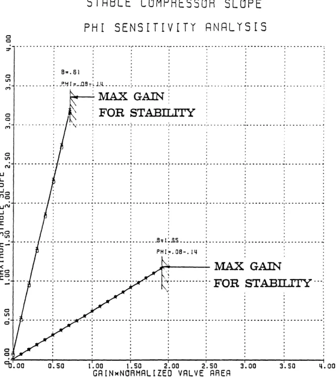
Choosing a y and 0 for a typical operating point near surge gives the nondimensional valve slopes with respect to flow coefficient and mean area. For a given B factor, the gain can be increased from zero to determine the threshold slope under those conditions at any value of zA . A sensitivity analysis is first
in V or ý. Figure (2.9) shows the results for 4 varying from 1.74 to 1.93 at a fixed value of
*
= .12. Two values for the B factor are examined: .61 and 1.65. These correspond to the experimental conditions to be discussed. The plot shows that the slope calculations are relatively insensitive to variations in the specified pressure rise. Similarly, a second plot (Figure (2.10)) shows the same analysis performed for fixed V = 1.87 with ý varying from .08 to .14. Again, mass flow variations have little effect on the tolerable slopes. Therefore the results for the selected representative point (V = 1.87 and 0 = .12) can be considered applicable to all speedlines since all surge points fall in this range. This will be seen in the data of Chapter 5.From both Figures (2.9) and (2.10), for a given B parameter, there exists a maximum compressor slope beyond which no amount of control gain can stabilize the system. Both this maximum slope and the corresponding zA to achieve stability under these conditions can be plotted as a function of B parameter.
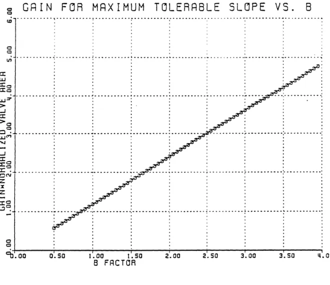
Figure (2.11) is the curve of maximum compressor slope for stability vs. B. From this plot, it becomes apparent that the controlled system (with the proper gain) can tolerate much steeper compressor characteristics at low B. The control is thus predicted to be more effective in the smaller B configurations. Figure (2.12) is the graph of required controller gain vs. B for the maximum tolerated slope. The gain is smaller at small B's, even though the system can tolerate steeper slopes than for high B parameters. This calculation highlights the B dependence of the system behavior with control.
For a general complex controller gain zA , the coefficients in the
characteristic equation (Eq. (2.20)) have both real and imaginary parts. The roots
of this equation in general are of the form:
s=
13
i(on (2.28)The real part of the poles, 5, is the growth rate of disturbances. For positive
3
any introduced perturbations will grow exponentially at eot. For negativegrowth rates, the perturbations are damped out exponentially. The imaginary
part of the roots, wn, corresponds to the natural frequency of the oscillations,
which may or may not be damped out. At zero gain this frequency is the
Helmholtz resonant frequency. If the real part of s is zero, the oscillations will be
purely sinusoidal and neutrally stable.
For a given magnitude of the controller gain, the pole positions will change as the phase of zA is varied, corresponding to a time lag between pressure
perturbations and the valve motion. Plots may be obtained for the growth rate
and natural frequency of the system at a constant gain magnitude as the phase is
swept from 0* to 360*. Figure (2.13) shows the variation in growth rate with
phase, normalized by the growth rate at zero magnitude (no control). Since the
selected operating point of
4
= .12 and y = 1.87 at B = .61 for this calculation isunstable without control, 00 is positive. Therefore, any portions of the curve
below the horizontal axis reflect a stabilization of the system by reduction in the
growth rate. Controller phases between zero and approximately 700 and between
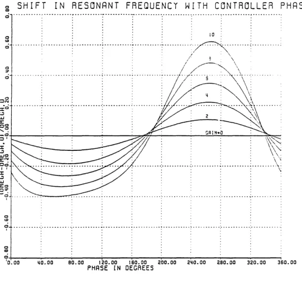
Increasing gain at zero phase moves the poles down to the real axis, where they remain at even higher gains. Thus at zero controller phase shift the natural frequency corresponding to the imaginary part of the poles is always reduced until (p - 0o)/0o = -1 corresponding to the poles lying on the real axis (Figure
(2.14)). At approximately 2000 and 3400 the resonant frequency remains virtually constant for any gain. Thus the poles are moved horizontally in the direction indicated by
f
in Figure (2.13). At 2000 phase shift the poles are pushed to the right for increasing gain, while at 3400 increasing gains tend to stabilize the poles. Finally, note that near 270* the frequency grows at larger gains while the growth rate remains the same. The poles are therefore moved vertically indicating no change in the stability of the system, only a change in the frequency of oscillation. These plots are analagous to those shown by Huang [9], even though the control law is different.2.4 Summary of Control Modelling
The central conclusions from the linearized compression system model are:
* The control scheme can stabilize the system in a nominally unstable region.
* Both the gain and the phase of the controller must be properly selected for the system parameters at a given operating point.
* There is both a minimum and maximum gain at any controllable operating point which will ensure stability.
* A controller phase of zero degrees is optimum. Some control may be achieved with nonzero phase, but the stable range of control gain is limited. A phase of 1800 can drive the system unstable even at nominally stable operating points.
* The B parameter and the slope of the compressor characteristic are the dominant influences on system stability.
* Implementing the controller affects both the perturbation growth rate and the resonant frequency of the system.
CHAPTER 3
Preliminary Results Using the Low Speed Test Facility
3.1 Low Speed Test Rig
The following section gives a brief outline of the low speed results with control. More detailed descriptions of the facility, instrumentation, and methodology will be presented in subsequent chapters which describe the high speed test rig.
The initial low speed data was obtained on a table-top test rig, consisting of a small diesel truck turbocharger manufactured by Holset and a plenum constructed from PVC plastic pipe. This main plenum, in conjunction with the compressor and its inlet ducting, resonated at its Helmholtz frequency of 22 Hz during mild surge.
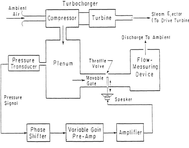
A gate valve at the plenum exit controlled the steady state throttling of the system. Downstream of this "fixed" valve was the controller: a gate mounted to the center cone of a Radio Shack 5 inch diameter loudspeaker. As a sinusoidal signal was sent to the loudspeaker, the moving coil drove the gate in an up and down motion to change the control throttle area. Air from the plenum exhausted through these valves into a second PVC pipe plenum which served as a mean mass flow measuring device.. An orifice was located at the exit of this second plenum, and the pressure drop across the orifice to ambient provided the flow measurement. The volume of this plenum was calculated so that the second plenum would be away from resonance at surge.
The main plenum was instrumented with a high response Setra pressure transducer connected to a static pressure tap. A static pressure tap was also located upstream of the second plenum orifice and connected to a 20 inch inclined alcohol manometer. A third static pressure tap was located approximately one pipe diameter from the bellmouth of the compressor inlet. This pressure drop, an auxiliary measure of the mass flow, was measured using a 20 inch Meriam manometer filled with .855 specific gravity fluid. A magnetic pickup at the impeller face provided a once per rev pulse to measure the turbocharger's rotational speed. Figure (3.1) shows a schematic of the low speed test setup and its associated instrumentation.
A closed-loop oiling system supplied 30W oil to the turbocharger bearings at 30 psig. The compressor was driven by using a steam ejector at the turbine exit with the turbine inlet open to ambient. Limitations of this drive system and the relatively low pressure and temperature ratings of the PVC restricted the maximum operating speed. A typical run was conducted at 30,000 RPM and the maximum speed at which data was taken was 60,000 RPM. 45,000 RPM was the minimum speedline on the map published by Holset for this turbocharger (Figure
(3.2)).
The signal from the high response transducer was fed through a phase shifter and pre-amplifiler, circuits for which are shown in Appendix B, and into a Harmon/Kardon model hk ultrawideband monophonic DC amplifier. The output of this amplifier drove the speaker to complete the control loop. The phase shifter has switchable ranges from 00 to 1800 and from 1800 to 3600 phase difference between input and output signals. The phase shifter also contains a high pass
filter to remove the pressure transducer DC signal, and it attenuates the incoming signal by a factor of 10. The pre-amplifier allowed the gain to be adjusted continuously from zero to approximately 100. The Harmon/Kardon amplifier boosted the signal to power levels adequate to drive the speaker.
3.2 Low Speed Test Results
To test the controller, the fixed valve was slowly closed down while maintaining a constant compressor rotational speed. The natural surge point was defined as the last observable operating point before flow reversal occurred. When surge was induced, the gain of the controller was increased from zero until the pressure fluctuations were suppressed. It was necessary to keep the controller on throughout the run because, if the controller were switched on or off, a spike in the gate motion resulted which was sufficiently energetic to induce surge. Therefore the- controller was left on at zero gain during the entire run until it was needed.
Linear theory predicts that the optimum phase difference between the plenum pressure fluctuations and the area fluctuations produced by the gate motion was near zero. The phase shifter was (empirically) adjusted to provide this phase under surge conditions. It was also noted that if the phase was adjusted to
1800 the controller would amplify small perturbations rather than suppress them.
Surge could thus be induced in a normally stable region of operation as well as intensified if the system was already in surge. The controller phase could be swept from 00 to 1800 and back again to alternately stabilize and destabilize the system.
Data taken at 30,000 RPM indicated that with simple proportional feedback, stabilization of the compressor could be achieved both at and below the natural
surge point. The controller set at 00 phase shift allowed the compressor to be
stably operated down to a flow coefficient of 50% of the flow coefficient at
uncontrolled surge, as shown in Figure (3.3). It was demonstrated that the
pressure rise vs. mass flow characteristic did not fall off to the left of the surge line, but rather followed a smooth contour. Thus the linear model could be used in the positively sloped region to predict the behavior of the system under control.
3.3 Conclusions
The preliminary data taken at low speed indicated that the proportional throttle control was a viable scheme, and the added stable operating region
provided by this method could be substantial. The success of the controller at the
low speeds suggested that control at realistic speeds would be feasible. To run at
high speed, however, a new facility would have to be constructed which could
withstand the higher temperatures and pressures. In addition a new control
valve would have to be designed because the speaker/moving gate could not overcome friction forces under high speed loading.
It was therefore proposed to build an new high speed facility which would
incorporate a fast response servomotor-actuated control valve. Sizing of the
system was done to achieve a range of realistic values for the B parameter at
110,000 RPM. A maximum B = 1.9 was selected to match the properties of an
existing aircraft engine centrifugal compressor at its design point [17]: Vp = 580
in3, Vc = LcAin = 91.7 in3, and Mtip = U/atip = 1.5. The system geometry was
simulate realistic conditions and to facilitate the sensing and actuation of the controller.
CHAPTER 4
High Speed Test Facility and Experimental Methods
4.1 Introduction
The test facility was designed to run the turbocharger at speeds near its
peak efficiency region, with 110,000 RPM selected as the design speed for the
controller. The high temperature and pressure rises associated with this speed were roughly 300*F and 15 psig. The facility was instrumented for both transient and steady state measurements, and all data acquisition was through a personal computer analog to digital interface. A throttle controller was specially designed for this application, including a rotary gate valve with its own position control loop as well as an outer system control loop. The next section gives an overall description of the facility; subsequent sections will describe the different components in more detail.
4.2 General Facility Description
The high speed facility consists primarily of four components, along with their associated support systems and instrumentation. A schematic is shown in Figure (4.1). First, the turbocharger, which is further described in Section (4.3), is driven on the turbine side by the lab oil-free compressed air line at the inlet and the steam ejector at the exit. Both lines are connected by flexible hose couplings. The compressed air system is capable of delivering 700 SCFM at 100
psig, and the line is provided with a gate valve to regulate flow along with pressure gauges on either side of the valve to monitor the delivery. The steam ejector line has a ball valve to regulate its outflow, but this is normally left wide open for maximum capacity. A bypass is provided to vent the compressed air to
atmosphere in case the vacuum is lost in the steam ejector line. This avoids overpressurizing the turbine housing.
Air enters the compressor side of the turbocharger through a bellmouth inlet, and exhausts through an exit duct to the second major component: the main plenum. The plenum is constructed of stainless steel and has two outlets. The first is through a ball valve at the bottom of the plenum. The second is through a flange mounted on the side of the plenum directly opposite the inlet tube. Only one exit is used at a time, depending on the control valve configuration. The duct from the compressor exit to the plenum extends through the inner diameter of the plenum to within several inches of the exhaust flange on the opposite side. The control valve was designed to mount either directly onto the end of this duct pipe or on the outside of the exhaust flange. In the first configuration (the compressor exit mode), the air delivered from the compressor must pass through the control valve before expanding into the plenum. The exhaust flange is capped off so that the outflow from the plenum is entirely through the ball valve at the bottom of the plenum. In the second configuration (the plenum exit mode), the air empties directly from the compressor exit duct into the plenum before passing out through the exhaust flange and subsequently the control valve. In this configuration the ball valve at the bottom is shut off so that all outflow is through the control valve. Another ball valve downstream of the control valve in the plenum exit mode allows steady state throttling in series with the control valve, if desired.
Both main plenum exit ducts connect to the final major component: the
second plenum. Also constructed from stainless steel pipe, this plenum serves as a
steady state mass flow measuring device. It contains flow straighteners to assure
a uniform exit profile and an orifice plate at the exit across which to measure the
pressure drop associated with the given flow rate. The flow exits the second
plenum through this orifice to atmosphere. These components are mounted in a
Unistrut stand, and the turbocharger is shielded in the radial direction by both a .375 inch thick aluminum plate and a layer of chain mail.
4.3 Turbocharger and Connecting Systems 4.3.1 Turbocharger Description
The turbocharger used in these experiments is a Holset model H1D
developed for diesel engines between 80 and 180 horsepower. The compressor has
an inlet duct inner diameter of 2.047 inches (5.2 cm). The impeller has an
annular inlet area of 1.938 inches2 (12.5 cm2) with a hub to tip radius ratio of .37,
and an exit tip diameter of 2.165 inches (5.5 cm). There are 6 blades, 6 splitter
blades, no inlet guide vanes, and a vaneless diffuser. The compressor exit duct is
1.732 inches (4.4 cm) inner diameter. A detailed exterior drawing and exploded
assembly drawing of the turbocharger are given in Figures (4.2) to (4.4).
The compressor is designed to operate up to a maximum total pressure ratio
of 3.1 at 140,000 RPM. At the selected design speed of 110,000 RPM for this
experiment, the maximum expected pressure ratio is 2.2. The reader is referred
again to Figure (3.2) for the compressor performance map supplied by Holset for
the impeller face; the output pulses are converted to Hertz by an HP 5316A Universal Counter.
4.3.2 Inlet Duct andl Instrumentation
4.3.2.1 Short Inlet Duct (Large B Configuration)
Two inlet ducts of different lengths were used to vary the B parameter as desired. The shorter duct was used for the large B configuration. This short inlet duct is constructed from PVC plastic and consists of a bellmouth inlet and an 8.9 inch (22.6 cm) long pipe of 2.04 inches (5.2 cm) inner diameter. The duct is instrumented with a two static pressure taps located at 00 and 270* measured clockwise from the top when viewing the duct from the bellmouth. Both taps are located 4.9 inches (12.4 cm) from the bellmouth inlet face and 4.0 inches (10.2 cm) upstream of the impeller face. A Type K unshielded thermocouple is inserted to
the center axis of the duct at 0° approximately .5 inches (1.3 cm) upstream from
the pressure taps to measure the inlet flow total temperature.
Inlet flow measurements with the short duct were obtained using a pressure signal from a transducer connected to one of the static pressure taps. The transducer is a Druck model PDCR 811 silicon strain gauge bridge transducer. Its operating pressure range is 0 to 2.5 psig with a full scale output of 25 millivolts at 10 volts excitation. The transducer output was amplified to approximately 10 volts full scale by an Analog Devices model 2B31L high performance strain gauge signal conditioner. This signal conditioning module provided programmable signal amplification and three-pole filtering as well as transducer excitation. The low-pass filter cutoff frequency was set at 500 Hz. The transducer and signal

![Figure 4.15 Motor Position Control Loop Schematic [13]](https://thumb-eu.123doks.com/thumbv2/123doknet/13843071.444114/130.918.142.806.256.515/figure-motor-position-control-loop-schematic.webp)