ASSESSMENT OF THE MODELING
ABILITIES OF NEURAL NETWORKS
by
Alvin Ramsey
Submitted to the Department of
Mechanical Engineering in Partial Fulfillment of the Requirements for the
Degree of
Master of Science in Mechanical Engineering
at the
Massachusetts Institute of Technology
January 1994
© Massachusetts Institute of Technology 1994 All rights reserved
Signature of Author ..lDpartment
/t
/ I Certified by -~~ '4ro essor 1 I , .l l
V~rto
of Mechanical Engineering January 1994 I ---George Chryssolouris Thesis Supervisor Accepted by...- ... - '-- Professor Ain A. Sonin
i A)-:S 1'!!
3NSr
Graduate CommitteeOF TFrHR A
-DEDICATION
To my mother ( o o3 )
and
to my brother ( Bro, on my word,
ASSESSMENT OF THE MODELING
ABILITIES OF NEURAL NETWORKS
by
Alvin Ramsey
Submitted to the Department of Mechanical Engineering on January 1994 in partial fulfillment of the requirements for the Degree of Master of Science in
Mechanical Engineering
ABSTRACT
The treatment of manufacturing problems, whether in process control, process optimization, or system design and planning, can be helped by input-output models, namely, relationships between input and output variables. Artificial neural networks present an opportunity to "learn" empirically established relationships and apply them subsequently in order to solve a particular problem. In light of the increasing amount of applications of neural networks, the objective of this thesis is to evaluate the ability of neural networks to generate accurate models for manufacturing applications. Various neural network models has been tested on a number of "test bed" problems which represent the problems typically encountered in manufacturing processes and systems to assess the reliability of neural network models and to determine the efficacy of their modeling
capabilities.
The first type of problem tested on neural networks is the presence of noise in experimental data. A method to estimate the confidence intervals of neural network models has been developed to assess their reliability, and the proposed method has succeeded for a number of the models of the test problems in estimating the reliability of the neural network models,
and greater accuracy may be achieved with higher-order calculations of confidence intervals
which would entail increased computational burden and a higher requirement of precision for the parametric values of the neural network model.
The second type of problem tested on neural networks is the high level of nonlinearity typically present in an input-output relationship due to the complex phenomena associated within the process or system. The relative efficacy of neural net modeling is evaluated by comparing results from the neural network models of the test bed problems with results from models generated by other common modeling methods: linear regression, the Group Method of Data Handling (GMDH), and the Multivariate Adaptive Regression Splines (MARS) method. The relative efficacy of neural networks has been concluded to be relatively equal to the empirical modeling methods of GMDH and MARS, but all these
modeling methods are likely to give a more accurate model than linear regression.
Thesis Supervisor: Professor George Chryssolouris
ACKNOWLEDGMENTS
Many deserves thanks and recognition for helping me develop the work performed for the Laboratory for Manufacturing and Productivity at MIT. I would like to thank my advisor, Professor George Chryssolouris, for his guidance, support, and opportunity to work in his research group. I must also thank Dr. Moshin Lee, Milan Nedeljkovic, Chukwuemeka (Chux) Amobi, and German Soto for their contributions to the work presented in this thesis; they are among the "buddies" of the lab. I like to thank the rest of the buddies: Subramaniam (the original Buddy), Andrew Yablon, Andrew Heitner, Sean Arnold, Eric Hopkins, Wolfram Weber, Johannes Weis, Giovanni Perrone, Dirk Loeberman, Ulrich Hermann, Helen Azrin, Tina Chen, and Steve Marnock.
And I finally would like to thank my mother, Kun Cha Ramsey, and my brother, Dan Ramsey, for their continuous support.
TABLE OF CONTENTS
LIST OF FIGURES ... 7
LIST OF TABLES ... 9
1. INTRODUCTION ... 10
2. NEURAL NETWORKS FOR EMPIRICAL MODELING ... 15
2.1. Empirical vs. Analytical Modeling ... 15
2.2. Neural Network Background ... 16
2.2.1. The Pursuit of Pattern Recognition ... 17
2.2.2. Backpropagation Neural Networks ... 19
2.2.3 Other Neural Network Architectures ... 22
3. NEURAL NETWORKS IN MANUFACTURING . ... 24
3.1. Areas of Applicability ... 24
3.1.1. Process Control, Diagnostics and Optimization ... 24
3.1.2. System Design and Planning ... ... 28
3.2. Current Applications of Neural Networks in Manufacturing ... 30
4. CONFIDENCE INTERVAL PREDICTION FOR NEURAL
NETWORKS
...
37
4.1. Confidence Intervals for Parameterized Models ... ... 37
4.1.1. Selection of the Variance-Covariance Matrix ... 40
4.2. Derivation of Confidence Intervals for Models Derived from Noisy Data ... 41
4.3. Derivation of Confidence Intervals for Neural Networks ... 43
5. APPLICATION OF CONFIDENCE INTERVAL PREDICTION FOR NEURAL NETWORKS ... ... 47
5.1. Test Problem: Multivariate Test Functions . ... 47
5.1.2. Neural Network Modeling of the Multivariate Test Functions ... 48
5.1.3. Neural Network Reliability ... ... 52
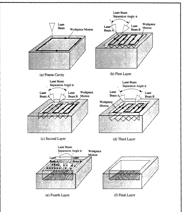
5.2. Test Problem: Laser Machining ... 53
5.2.2. Neural Network Modeling of Laser Through-Cutting ... 56
5.2.2. Neural Network Modeling of Laser Grooving ... 57
5.2.3. Neural Network Reliability ... ... 59
5.3. Test Problem: The Manufacturing of an Automobile Steering Column ... 59
5.3.1. An Evaluation Framework for Manufacturing Systems ... 60
5.3.2. The Manufacturing of an Automobile Steering Column ... 62
5.3.3. Neural Network Modeling of the Manufacturing of the Steering Column ... 70
5.3.4. Neural Network Reliability ... ... 71
6. RELATIVE PERFORMANCE OF NEURAL NETWORKS ... 73
6.1. Linear Regression ... 73
6.2. Group Method of Data Handling ... 74
6.3. Multivariate Adaptive Regression Splines ... ... 78
6.3.1. Recursive Partitioning Regression . ... 79
6.3.2. Adaptive Regression Splines ... ... 80
6.4. Results of the Various Modeling Approach to the Test Bed Problems ... 81
6.4.1. Modeling of the Multivariate Test Functions ... 82
6.4.2. Modeling of Laser Machining ... .... ... ... 85
6.4.2.1. Laser Through-Cutting ... 85
6.4.2.2.
Laser
Grooving
...
...
.. ... 86
6.4.3. Modeling of the Manufacturing of an Automobile Steering Column ... 87
6.4.4. Overall Assessment of the Relative Modeling Efficacy of Neural Networks ... 89
7. CONCLUSION ... 900... 7.1. Use of Confidence Intervals to Assess Neural Network Reliability ... 90
7.2. Relative Efficacy of Neural Network Models ... 91
7.3. Summary ... 92
LIST OF FIGURES
Figure Figure Figure Figure Figure Figure 2.1: 2.2: 2.3: 2.4: 4-1: 5-1: Figure 5-2: Figure 5-3: Figure 5-4: Figure 5-5: Figure 5-6: Figure 5-7: Figure 5-8: Figure 5-9: Figure Figure Figure 5-10: 5-11: 5-12: Figure.5-13: Figure 5-14: Figure 5-15:Example of a linearly separable pattern ... 1... 18
The exclusive OR problem ... 1... 19
An example of a feedforward neural network ... ... 20
A 1-1-1 neural network with linear input and output nodes ... 22
A 1-1-1 neural network with linear input and output nodes ... 43
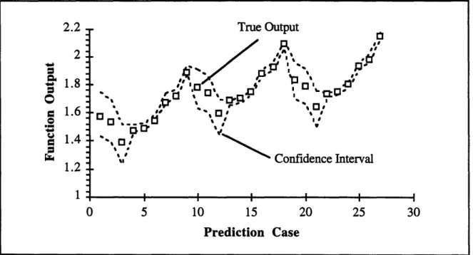
806% confidence intervals for the neural network model of function 1 ... 49
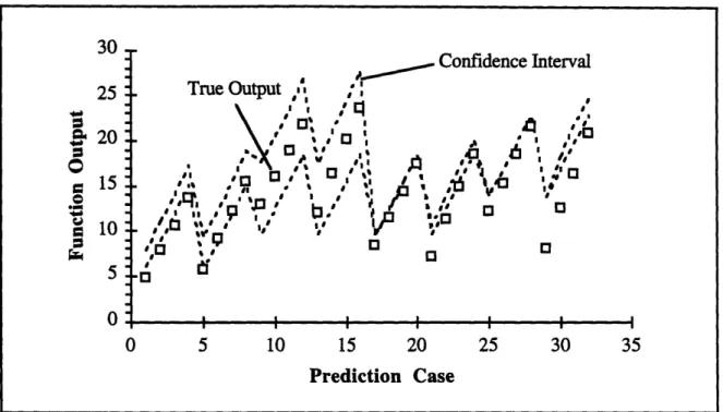
800% confidence intervals for the neural network model of function 1 containing noise ... 49
806% confidence intervals for the neural network model of
function
2 ...
...
...
...51
80% confidence intervals for the neural network model of function 2 containing noise ... 51
Laser through cutting ... ...54
Using three-dimensional laser grooving for ring removal ... 55
Using three-dimensional laser grooving for milling ... ... 56
80% Confidence intervals for the neural network model of laser cutting ... ... ... 58... 58
80% Confidence intervals for the neural network model of laser grooving ... 59
Configuration of a manufacturing system ... 61
Summary of total life cycle costs ... 62
Schematic of the automobile steering column (hazard switch and tilt lever are not shown). ... 64
Convention for setting buffers. ... 69
80% confidence intervals for the neural network model predictions ... 70
80c% confidence intervals for the neural network model predictions trained from noisy data ... 71
The second generation output y as a function of the input
parameters xi, xj, xk, and xl ... 76
A complete GMDH model, showing the relationship between the input variables and the output y ... ... 76
Steps to develop the GMDH algorithm ... ... ...78
The MARS forward algorithm... 81
Comparison of results of the different models of Equation (5-1) ... 83...83
Comparison of results of the different models of Equation (5-1) containing noise ... 83
Comparison of results of the different models of Equation (5-2) ... 84
Comparison of results of the different models of Equation (5-2) containing noise ... ... 85
Comparison of results of modeling laser through-cutting ... 86
Comparison of results of modeling laser grooving ... ... 87
Comparison of results of modeling the manufacturing systems ... 88
Comparison of results of modeling the manufacturing systems with noisy data ... 88
Figure 6-1: Figure 6-2: Figure Figure Figure 6-3: 6-4: 6-5: Figure 6-6: Figure 6-7: Figure 6-8: Figure Figure Figure Figure 6-9: 6-10: 6-11: 6-12:
LIST OF TABLES
Table 5-1: Summary of the predictions which lie within the 80% confidence intervals and accuracy of fit for the models
to the training data ... ... ... 52... 52
Table 5-2: Available resource types and required tools for processing the tasks ... 65
Table 5-3: Costs of resources ... 66
Table 5-4: Additional information for calculating the efficiency ... 66
Table 5-5: Task data per model ... ... ... 67...67
Table 5-6: Tardiness cost rates and inventory carrying costs ... 67
Table 5-7: Summary of the predictions which lie within the 80%
confidence
intervals
...
...
... 71
CHAPTER 1
INTRODUCTION
A large variety of manufacturing processes are used in industrial practice for transforming material's shape, form, and properties. In the metalworking industry, there are more than 200 well established processes used for such purposes [Chryssolouris, 1992]. Modeling of manufacturing processes refer to the creation of the set of relationships that relate input to the process and its outputs. Such descriptions of manufacturing processes are very
useful in terms of optimizing the process as well as in terms of controlling it. Very often in
industry, the lack of an adequate process model leads to extensive trial and error experimentation, suboptimal processes, and waste of material, labor, and energy.
Manufacturing problems, whether in process control, process optimization, or system design and planning, can be solved only with the help of appropriate models, namely, some sort of a relationship between input and output variables. Such a relationship can be
constructed either analytically, on the basis of analysis of the interactions between the input
variables, or empirically, on the basis of experimental/historical data. For manufacturing problems, the analytical route is often difficult to take because the relevant input-output relationship may be a product of many complex and interacting phenomena. For this reason, over the past years, researchers active in the field of manufacturing have pursued a variety of empirical approaches to manufacturing modeling. The main drawback of these approaches is that they have relied on regression techniques, which require an a priori knowledge of the general algebraic form of the input-output relationship. While such knowledge may be available for particular manufacturing problems, it is very difficult to generalize to other problems.
The analytical route in solving manufacturing problems in process optimization, system design and planning, and process control is often difficult to take because the relevant input-output relationship may be a product of many complex and interacting phenomena. The advent of neural networks presents an opportunity to overcome this difficulty for manufacturing problems.
Modeling of many manufacturing processes often involves an extensive analysis of a physical behavior of the process to derive a mathematical model. Creating a precise and accurate model of the manufacturing process often results in a model which requires a sizeable amount of computation. Simplifying a model to reduce the computational size sacrifices the accuracy of the model. When developing a model for a manufacturing process, accuracy conflicts with workability. A modeling technique for manufacturing processes which can compromise the characteristics of an accurate and a manageable model is needed. A possible approach involves the use of artificial neural networks, which is a
computational tool used in artificial intelligence.
There are two specific classes of problems in manufacturing where neural networks can be
applied:
* The first class of problems involves process diagnostics, process control, and process optimization. Most control schemes for manufacturing processes use a single sensor to monitor a machine or a process. In many cases, this approach is inadequate primarily due to inaccurate sensor information and the lack of a single process model
which can sufficiently reflect the complexity of the process.
· The second class of problems involves manufacturing system design and planning. The design of a manufacturing system can be viewed as
the mapping of the system's performance requirements onto a description of a system which will achieve the required performance.
Presently, there are only few, highly specialized methods which support
such a mapping process, and due its the complexity, global optimization
cannot be obtained effectively by trial-and-error methods. System designing normally compromise between quality of the solution and design effort.
Current applications include the development of neural network technology for manufacturing applications, particularly related to process diagnostics, control, and
optimization, as well as to system planning and design. A new approach to process control
and optimization is to synthesize the state variable estimates determined by the different sensors and corresponding process models using neural networks. For system design and planning, neural networks can be used to provide an efficient method of supporting the optimization of a manufacturing system design in a "closed loop" by learning from selected "experimental" values (can be obtained by simulation) which show the interdependencies between decision variables and performance measures. Neural networks can therefore be
seen as catalysts for greater CIM capability.
In light of the increasing amount of possible applications of neural networks, the objective of this thesis is to evaluate the ability of neural networks to generate accurate models of physical systems typically encountered in manufacturing. By determining the reliability of neural network models and by comparing the efficacy of neural networks with other methods of empirical modeling as criterions, an assessment of the modeling abilities of neural networks can be formed.
Various neural network models will be tested on a number of "test bed" problems which represent the problems typically encountered in manufacturing processes and systems to determine the efficacy of their modeling capabilities. The problems chosen for the test bed
are the following:
* two arbitrary multivariate functions
· laser through-cutting and laser grooving
· the manufacturing system design of an automobile steering column.
The first type of problem to be tested on neural networks is the presence of noise in experimental data. Systems have error associated with it due to the dependence of the
output on uncontrollable or unobservable quantities, and the quality of the model developed
from data containing such errors will be compromised to a certain degree. A method to estimate the confidence intervals of neural network models will be developed in order to assess their reliability. For a desired degree of confidence (i.e., for a given probability), a
confidence region can be calculated for a parameterized model. Treating the neural network
as a parameterized model, the confidence intervals can be estimated with this approach.
The second type of problem to be tested on neural networks is the high level of nonlinearity
typically present in an input-output relationship due to the complex phenomena associated within the process or system. The relative efficacy of neural network modeling will be determined by comparing results from the neural network models of the test bed problems with results from models generated by other common empirical modeling approaches: linear regression., the Group Method of Data Handling (GMDH), and the Multivariate Adaptive Regression Splines (MARS) method. The GMDH is a modeling technique that groups the input variables in a form of a polynomial regression equation to predict the
which combines recursive partitioning (the disjointing of the solution space for the model
into different subregions) and spline fitting.
By exploring these two types of problems applied to the test bed problems mentioned, an assessment of the modeling abilities of neural networks can be formed. Following the introduction, Chapter 2 will provide an overview of neural networks. Chapter 3 will cover current applications of neural networks in manufacturing. Chapter 4 will explain the proposed method of estimating confidence intervals for neural networks. Chapter 5 will
provide the results in estimating confidence intervals on neural network models. Chapter 6
will provide the results in comparing the relative efficacy of neural networks. Finally, the
CHAPTER 2
NEURAL NETWORKS FOR EMPIRICAL MODELING
Throughout various industries, such as the manufacturing and chemical industries, artificial
neural networks have been successfully used as empirical models of processes and systems. This chapter will begin by discussing the advantages and disadvantages of empirical modeling versus analytical modeling. An introduction to artificial neural networks for empirical modeling follows, then the chapter will conclude by overviewing
the current uses of artificial neural networks for industrial applications.
2.1. Empirical vs. Analytical Modeling
Analytical modeling of physical systems is the development of a mathematical expression for the system based on knowledge of the physical phenomenons occurring within the system. In general, development of an analytical model of a system entails simplification of the true behavior to make possible the arrival of a manageable and tractable solution,
where often the simplification is a gross assumption which can produce enormous errors in
the model. After making simplifications and assumptions of the system to arrive to an analytical model representing the physical system, there is still no guarantee that the analytical approach to obtain a model can be used. Although the advent of high speed processors for computers make numerical methods for solving highly complex and nonlinear functions possible, the amount of time required to solve such functions may still be too much for on-line use of models, such as those used for on-line plant monitoring and control. Another reason that analytical models may not be useful is that the simplifications and assumptions required to develop the model may cause gross errors in the predictions, thus making the model useless.
Empirical modeling of physical systems is the development of a model based on experimental observations and either interpolating or extrapolating the behavior of the system outside of the conditions given in the prior observations. Empirical modeling does not necessarily depend on a knowledge of the physical phenomenons that determines the behavior of the system, which can make empirical modeling the better (or sometimes the only) option in modeling. Empirical modeling requires the proper amount of "adequately" distributed observations of the physical behavior of the system, which is not always
possible to obtain. If the cost of obtaining each experimental observation is relatively large,
then the adequate amount of observations may be too costly to obtain. Also, some a priori knowledge of the physical phenomenons which determines the behavior of the system is
required in order to determine the parameters necessary to include in the model because the
inclusion of parameters which has no bearing on the behavior of the system can produce an invalid model.
When trying to obtain a model to predict a behavior of a system, the analytical approach would be the ideal approach, but if the cost and effort causes this approach to be either impractical or impossible, the empirical approach would be either the better or only choice. The benefits, along with the shortcomings, of the two approaches must be weighed when
selecting the modeling approach.
2.2. Neural Network Background
According to Hecht-Nielsen, neurocomputing is the technological discipline concerned with
parallel distributed information processing systems that develop information processing capabilities in response to exposure to an information environment [Hecht-Nielsen, 1990].
Neural networks are the primary information processing structures of interest in
neurocomputing. The field of neural networks emerged from the developments of the neurocomputers, and today, development and implementation of neural networks span
across the boundaries of neurocomputers and cross into numerous disciplines for many different applications. The evolution of neural networks can be traced back to approximately half a century, which reveals the amount of history behind the relatively new field of neural networks.
2.2.1. The Pursuit of Pattern Recognition
The work which lead to the 1943 paper "A Logical Calculus of the Ideas Immanent in Nervous Activity" by McCulloch and Pitts has been credited by many to be the beginning of neurocomputing [McCulloch and Pitts]. This work inspired the concept of a "brain-like" computer, but the concept was purely academic and there were no direct practical applications suggested. The developments of the network which uses the Adaptive Linear Element (ADALINE) by Widrow and the perceptron network by Rosenblatt in the late 1950's produced some of the first useful networks [Widrow][Rosenblatt].
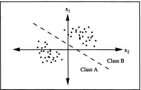
Rosenblatt's primary interest was pattern recognition. He invented the perceptron, which is a neural network that had the ability to classify linearly separable patterns. Figure 2.1 illustrates two linearly separable patterns (classes A and B). The patterns are a function of the two inputs xl and x2, and because a straight line is able to distinguish the class of the outputs of xl and x2, the produced pattern is said to be linearly separable.
X1 0 0. 0 * · * 0so0 0 *·· 00 0 * o .@ . _%> X2 N% >Class B Class A
Figure 2.1: Example of a linearly separable pattern.
The perceptron did not have the ability to identify patterns which were not linearly separable, and this weakness was pointed out by Minsky and Papert [Minsky]. The famous example used by Minsky and Papert was the exclusive OR (XOR) problem. The XOR is a two input function with binary inputs which gives a binary output when only one of the inputs are on, either (1, 0) or (0, 1). If both are on (1, 1) or off (0, 0), an output would not be given. Figure 2.2 illustrates how the XOR problem is not linearly separable.
No line can separate the O class and the X class.
Work done by Rumelhart, Hinton, and Williams [Rumelhart] in 1986 demonstrated how a
network can develop a mapping which separates the two classes. The network architecture
contained hidden processing units, or nodes, which allowed nonlinear input-output mapping. By solving the XOR problem, the possibilities of neural networks to learn the
xl
Figure 2.2: The exclusive OR problem.
2.2.2. Backpropagation Neural Networks
According to Hecht-Nielsen [Hecht-Nielsen, 1990], a neural network is a parallel, distributed information processing structure consisting of processing elements (which can possess a local memory and can carry out localized information processing operations) interconnected via unidirectional signal channels called connections. Each processing element has a single output connection that branches ("fans out") into as many collateral
connections as desired; each carries the same signal - the processing element output signal.
The processing element output signal can be of any mathematical type desired. The information processing that goes on within each processing element can be defined arbitrarily with the restriction that it must be completely local; that is, it must depend only on the current values of the input signals arriving at the processing element via impinging
connections and on values stored in the processing element's local memory.
Although the definition of a neural network given is to some extent restrictive, the possible architectures for a neural network vary widely. A commonly used network architecture is the feedforward neural network. The structure of the feedforward neural network is a
i k
.4
0
l
connection of nodes arranged in hierarchical layers. The first layer contains the nodes which accept the input signals and send these signals to the nodes in the next layer through the connections (also known as links). The links from the nodes in each layer are connect
to the nodes in the following layer up to the final layer, where the input signals are sent in a
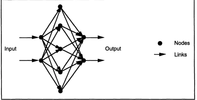
feedforward manner from the input layer to the output layer. Weight values are associated with each link which can be "corrected" to allow learning for the network. Figure 2.3 gives an illustrative example of a feedforward neural network. The unidirectional flow of the signals from the input to the output nodes classify this network structure as a feedforward neural network, but network structures classified as recurrent neural networks permit signals to flow to nodes within the same layer and to nodes in a previous layer in addition to the forward direction of flow.
Input
0
NodesOutput
Links
Figure 2.3: An example of a feedforward neural network.
Learning (also called training) is the process of conforming a neural network to map an input-output relation, where for a feedforward network, the conformation is the correction to the weight values to generate the correct input-output relationship. A common learning
algorithm for feedforward networks is the error-backpropagation algorithm, which iteratively corrects the values of the weights by propagating an error signal backwards from the output layer to the input layer. Feedforward networks trained by the
error-backpropagation algorithm are also known as error-backpropagation networks.
The outputs from a neural network are a conglomeration of nested nodal functions, and the sigmoidal function is a common choice for the nodal function. The mapping accuracy can be increased by introducing bias values to each nodes, which can also be viewed as a constant input to a node in addition to the inputs from the nodes in the previous layer. Equation (2.1) gives the sigmoidal function for a typical neural network with biases, and Equation (2.2) gives the neural network function for the simple 1-1-1 structure shown in Figure 2.4, where the input and output nodes implement linear functions and the middle node implements the sigmoidal function. The node in the second layer illustrates the sigmoidal function.
I + exp(-w-x+ b) (2.1)
Y = W2
1 I )+b 2
Layer 1 Layer 2 Layer 3
Figure 2.4: A 1-1-1 neural network with linear input and output nodes.
2.2.3. Other Neural Network Architectures
As opposed to supervised learning for multilayer perceptrons, the self-organizing network corrects itself by reading in only the input. This network has several links connecting the input and the output layer, but unlike the perceptron, there are recurrent links which connect the output nodes, or units, which composes the final layer. The input data is read, and the network determines the link with the least distance (the difference between the weight of the link and of the input value) and assigns the the region of the output node with the least distance to the input node. The trained network consists of an input-output layer, where the nodes of the output layer have been properly associated with its respective input nodes. In essence, the self-organized network is a heuristic lookup table, which is optimal for pattern identification used in speech and vision recognition, but is not as efficient for
function mapping as the multilayer perceptron [Hecht-Nielsen, 1990][Lippmann].
The counterpropagation network, devised by Robert Hecht-Nielsen, is a synthesis of the self-organizing network and the Grossberg learning network, which is a network consisting of multiple input-output nodes with weighted links that are adjusted by the Grossberg Learning Law [Hecht-Nielsen, 1990]. An assessment of this network given by
y
b /
2
its creator reveals that the network is optimal for real-time analysis and implements an algorithm similarly used for pattern classification for mapping functions, but a direct comparison to a multilayer perceptron reveals its weakness in generalization, due to its
CHAPTER 3
NEURAL NETWORKS IN MANUFACTURING
In this chapter, a discussion of the industrial applications for neural networks is given. The chapter will begin by addressing the areas of applicability in manufacturing for neural networks and will conclude by overviewing the current applications of neural networks in manufacturing.
3.1. Areas of Applicability
There are two specific classes of problems in manufacturing where neural networks can be applied. The first class of problems involves process diagnostics, process control, and process optimization, and the second class of problems involves manufacturing system design and planning. This section will discuss the applicability of neural networks in these two classes.
3.1.1. Process Control, Diagnostics and Optimization
Most control schemes for manufacturing processes use a single sensor to monitor the process. In many cases, this approach is inadequate primarily due to inaccurate sensor information and the lack of a single process model which can sufficiently reflect the
complexity of the process. As an alternative to the typical approach to process monitoring,
a multiple sensor approach which is similar to the method a human uses to monitor a manufacturing process can be implemented with neural networks. In such an approach, the measurement of process variables is performed by several sensing devices which in turn feed their signals into different process models which contain mathematical expressions based on the physics of the process.
Synthesis of sensor information can provide a number of benefits for process monitoring as opposed to the current state of the art approach of using a single sensor. This is
especially so for processes and systems that are difficult to model and monitor.
A considerable amount of work regarding the control of the manufacturing equipment and processes has been done over the past two to three decades. A major effort has been
focussed on applying the scientific principles of control theory to manufacturing processes.
Despite the high quality of work in this area, it appears that in reality the vast majority of manufacturing processes remain uncontrolled or empirically controlled due to the lack of two necessary elements for applying control theory principles to the control of manufacturing processes. The first element corresponds to sensing devices that will be
robust and reliable enough to provide the necessary signals from the manufacturing process
and/or equipment. The second element corresponds to comprehensive process models that
will reflect the complexity of the manufacturing process.
Numerically controlled machine tools generally use predetermined parameters such as feed
and speed as well as an open-loop control system, which has as inputs the machining parameters normally determined off-line during the process planning stage. These parameters are often determined with the aid of tables, machineability standards, and experience. Due to the fact that these parameters are determined well before the actual manufacturing process occurs, there is no way that automatic adaptation to the actual process can be achieved. Since factors disrupting the process are, for the most part, unpredictable, the choice of machining parameters must be made in such a manner that production is executed without breakdowns, even under the worst possible circumstances. Consequently, the capabilities of the machine are not fully utilized, and the manufacturing process is not efficient. Whenever adaptation to the actual situation or requirements of the
Adaptive control schemes for the machining process have been researched over the past twenty years. In Adaptive Control Constraint (ACC), the goal of the controller is generally to adjust the machine tool's setting parameters in order to maintain a measured quantity, such as the cutting force, at a specified value. ACC controllers are primarily based on closed-loop control theory. In its most basic form, this scheme has a single input and single output and employs fixed proportional and integral control gains. For the machining process, the input may be the feed rate or cutting speed and the output may be the cutting force. More complex schemes adjust the controller gains on-line in order to improve the control performance. Regardless of the complexity of the scheme, the goal is usually to drive a measured or estimated state or set of states to a desired set point. The general drawback of any ACC system is that maintaining a variable such as the cutting force at a
given set point will generally not optimize the process. Indeed, the significant optimization
objectives for machining are generally a function of the tool wear and wear rate as well as the process input parameters, rather than direct functions of measured process variables such as the cutting force or tool temperature. Functions relating these objectives with a measured quantity, such as the cutting force, would undoubtedly be very complex and nonlinear, since the cutting process is highly nonlinear. The optimization objectives may not even be a monotonically increasing or decreasing function of the process input parameters. This characteristic is in sharp contrast with standard transfer functions used in linear control design, where provided the system is stable, the quasi-static output of the plant is assumed to be a linear function of the input. In addition, linear control design is primarily effective for time-invariant systems, while the machining process is a complex time-varying system. Furthermore, linear control theory was primarily developed to maintain an objective at a specified set point; however, the goal of a process optimization scheme is not to maintain an objective at a preset value, but rather to obtain the maximum (or minimum) of the objective over the feasible range of process input parameters. For
these reasons, classical and modern control theory can be rendered inadequate for
optimizing not only the machining process but manufacturing processes in general.
Adaptive Control Optimization (ACO) schemes have been researched in an effort to optimize the machining process. The major obstacles to successful in-process optimization of machining operations have been the lack of sensing devices that can reliably monitor the process and the lack of a single process model which can comprehensively reflect the complexity of the machining process. With a few exceptions, most machining control schemes use a single sensor to monitor the process and therefore consider a single process model. Past research has shown that accurate process models are difficult to build and are generally unreliable for machining control over a wide variety of operating conditions. In contrast, if information from a variety of sensors and sensor-based models is integrated, the maximum amount of information would be used for making control decisions and thus the quality of the decisions would likely be better than decisions based on information from a single sensor. Ideally, different sensor-based models should provide the same estimates for the machining parameters. However, these estimates would generally include a significant amount of random noise. Utilizing several simultaneous sensor-based estimates can be considered analogous to taking several samples from a random distribution. Statistically, as more samples are taken, the confidence interval for the mean becomes narrower. In the same way, as more sensor-based model estimates are considered, the estimates for the machining parameters become more certain; the uncertainty due to randomness in the estimates is reduced. In addition, if one sensor fails during the process, a controller utilizing multiple sensors could probably continue to operate, while a controller
3.1.2. System Design and Planning
Particularly in the metal working industry, parts usually spend 5 percent to 15 percent of their time on the machinery and the rest of the time they move around on the factory floor waiting for machines, transportation, etc. This leads one to believe that decisions that are made regarding the design and operation of a production system can be vastly improved if one can establish a framework for decisions in this environment and optimize it from a total performance point of view.
A number of approaches have been proposed in the literature for the design of manufacturing systems. Usually, the overall manufacturing system design problem is decomposed into sub-problems of manageable complexity, meaning that only a single type of decision variable and a single type of performance measure is considered for each sub-problem.
* One sub-problem is the resource requirements problem. For this
problem, the task is to determine the appropriate quantity of each type of
production resource (for example, machines or pallets) in a manufacturing system.
* The resource layout problem is the problem of locating a set of
resources in a constrained floor space.
* In material flow problems, the objective is to determine the
configuration of a material handling system.
* The buffer capacity problem is concerned with the allocation of work in
These sub-problems are usually treated separately. This neglects the inter-relationships that exist between the different sub-problems (e.g., the required buffer capacity at a work center
in a manufacturing system depends on the number of machines in that work center).
Solution of this problem requires knowledge of the relationship between the performance measures and the decision variables. This relationship is highly nonlinear and difficult to establish for a number of reasons:
* Manufacturing systems are large-scale systems with many interacting components.
* The parameters which are responsible for the behavior a manufacturing system (e.g., processing times), are often uncertain and must be
characterized by distributions rather than constant values.
Existing methods address the difficulty of manufacturing system design by simplifying the problem definition. Common strategies for doing so are:
* Restrict the structure of the material handling system. Many approaches, for example, apply only to transfer lines, which have
purely serial material flow.
* Restrict the scheduling policies of the manufacturing system to simple rules which are easier to characterize mathematically (e.g., first come, first served).
* Consider only one fixed type of decision variable (e.g., buffer capacity) and one fixed performance measure (e.g., production rate) that can be easily expressed in terms of the decision variables.
Most control schemes for manufacturing processes use a single sensor to monitor the process. In many cases, this approach is inadequate primarily due to inaccurate sensor information and the lack of a single process model which can sufficiently reflect the
complexity of the process. As an alternative to the typical approach to process monitoring,
a multiple sensor approach which is similar to the method a human uses to monitor a manufacturing process, can be implemented with neural networks. In such a approach, the measurement of process variables is performed by several sensing devices which in turn feed their signals into different process models which contain mathematical expressions based on the physics of the process.
In manufacturing, the primary decision-making tools for system design remain simulation and analytical modeling. Each tool has a major weakness when it comes to the design of complex manufacturing systems: simulation suffers from excessive computational expense, while analytical modeling can be applied only to a very restricted subset of systems (e.g., systems such as transfer lines with purely serial material flow or systems with constant work in process). The approach using neural networks can accommodate manufacturing system design problems in which the performance requirements involve multiple types of performance measures (e.g., production rate and average work in process), and in which design solutions involve multiple types of decision variables (e.g., machine quantities and machine layout and buffer capacities).
3.2. Current Applications of Neural Networks in Manufacturing
Neural networks have been used for many types of manufacturing application. In general, input variables which affect the output of a manufacturing process or system are known, but the input-output relationship is either difficult to obtain or simply not known. Neural networks have served as a heuristic mapping function for various input-output
relationships. In this section, an overview of industrial applications of neural networks is given.
Neural networks have modelled the Electric Discharge Machining (EDM) process [Indurkhya, Rajurkar]. EDM is a process by which high strength temperature resistant alloys are machined by a very hot spark emanating from the tool to the workpiece across a dielectric fluid medium. Presently, the relationships between the controllable inputs and output parameters of the EDM process have not been accurately modelled due to their complex and random behavior. A 9-9-2 backpropagation neural network has been developed as the structure, where the nine inputs correspond to the machining depth, tool radius, orbital radius, radial step, vertical step, offset depth, pulse on time, pulse off time, and discharge current, which determines the two output parameters material removal rate and surface roughness. The neural network model proved to be closer to the actual experimental results when compared to multiple regression.
Neural networks have also been implemented to model the grinding operation. Standard automated control was not possible due to the fact that there are so many factors which affect the grinding process. Thus, the standard approach to control the grinding process was the employment of a skilled operator who relies on considerable experience to dynamically adjust the conditions to achieve the desired quality. A hybrid neural network have been implemented for the decision-making model of the process [Sakakura, Inasaki]. The hybrid model consists of a feedforward neural network and a Brain-State in a Box (BSB) network. The feedforward net serves as the input-output model of the grinding process, and the BSB net, which functions as a classifier similar to the associative memory of humans, serves to recall the most suitable combination of the input parameters for the desired surface roughness.
Neural networks have been used to model arc welding. The arc welding process is a nonlinear problem, which makes this process difficult to model. Full automation of this process has not yet been achieved due to the lack of knowledge of some of the physics in arc welding. A backpropagation neural network has been used to model the arc welding process as a multivariable system [Anderson, et al]. The outputs of the arc weld model were the bead width and bead penetration, which help to define the characteristics of the finished weld. The inputs of the model were the workpiece thickness, travel speed, arc current, and arc length, and the model gave prediction errors on the order of 5% or less. Some of the current works in this topic includes the implementation of a neural network
model for on-line control of the arc weld process.
Quality control of the injection molding operation has been implemented using a backpropagation neural network [Smith]. The input parameters of the model based on the equipment set-up were the temperatures of the four barrel zones along with the gate, head, and die zones. The input parameters based on the runs were the screw speed, DC power,
the line speed, the quench temperature, and the head pressure. Other independent variables
used for the model were the die and tip diameters, the air pressure, and the time of each sample since the line went up. A total of 16 input parameters were used to determine the two output parameters, which were the mean and variance of the injection molded piece. Results found were that neural networks perform comparably with statistical techniques in goodness of output for process and quality control. The neural network performed comparatively better when modeling quality/process control data which exhibits a nonlinear behavior.
The predicting of wire bond quality for microcircuits has been aided with neural networks [Wang, et al]. Wire bonding is the process by which a gold wire, where the thickness is in the order of 0.001 in., is "thermosonically" welded to to a gold or metal oxide pad in the
microcircuit. The costly testing of wire bond quality is traditionally implemented by the wire pulling test, and neural networks would serve as a low-cost approach to process control. The results show that the neural network can be used as an accurate and inexpensive alternative for predicting wire bond quality.
Wave soldering has been another process which neural networks attempted to model [Malave, et al]. The preheat temperatures and the conveyor speed are two of the machine parameters determine the bond quality, where a total of 26 input parameters affect the machine parameters. The neural network was not able to converge to a working model of the system, but the inability of the neural network to converge has been traced to faulty data. The data were collected randomly; no design of experiments were implemented to ensure a proper representation of the physical system.
CMAC (Cerebella Model Articulation Controller) has been integrated with neural networks for fault predictions in machinery during the manufacturing process [Lee, Tsai]. Through statistical process control (SPC), future values and estimations of machine performance are
calculated from the derived performance model, but these are only superficial models of the
system. Through the aide of a CMAC, a network can be created with the ability to detect faults by monitoring the output patterns from sensors and actuators. Thus by analyzing the timing sequence, abnormal conditions in the machinery become detectable. The CMAC model is a table-look up technique that provides an algorithm for random mapping of a large memory space to a smaller, practical space. From the mapping, nearby states tend to occupy overlapping memory locations and distance states tend to occupy independent memory locations. This scheme provides a form of linearization between nearby input vectors. The CMAC is not a method to process inputs into accurate outputs, but rather a model for real-time control that a biological organism appears to follow, i.e., in problem
for a response with the conditions at hand; after that, the situation is reassessed for the next action. The important point is that the organism has the capability to generate outputs
continuously and that each new output moves the organism in the correct direction closer to
the goals. CMAC offers the advantage of rapid convergence, and integrated with neural networks, allows the classification of failure based on pattern recognition by comparing the
input with that of a healthy subsystem to provide an indication of distress conditions.
Neural networks have been used as predictive models, but neural networks are also appropriate for the control and optimization of plant dynamics. In supervisory optimization, the optimizer (an expert) would make suggestions to the operator on how to
change the operating parameters of the plant so as to maximize efficiency and yet maintain a
smoothly running plant. When asked, it sometimes might be difficult for the expert to explain his reasons for altering certain parameters on the plant. This kind of expertise comes from experience and is quite difficult to incorporate into classical models or rule-based systems, but is readily learned from historical data by a neural network [Keeler]. The neural networks can provide several useful; types of information for the plant engineer,
including:
a) Sensitivity analysis
b) Setpoint recommendations for process improvement
c) Process understanding
d) Real-time supervisory control
e) Sensor validation - the neural networks can learn the normal behavior of sensors in a system and can be used to validate sensor readings or alarm for sensors that are not functioning properly.
f) Predictive maintenance - the neural networks can be used to predict component failure so as to schedule maintenance before the failure occurs.
As an adjunct technology to neural networks, fuzzy control is useful for implementing default rules for data poor regions. In addition, fuzzy rules are useful at the data analysis stage for screening data, at the modeling stage for describing behavior outside the data region, for incorporation of constraints, and for generation of fuzzy rules describing plant behavior and optimization procedures. Thus, fuzzy rule systems are ideal for bridging the gap between the adaptive neural network systems and hard rule-based expert systems.
The steps taken for the application of neural network technology to plant dynamics are:
1) Extract data from the historical database and store files,
2) Examine the data graphically and screen out any bad data points or outliers.
3) Estimate the time-delays of the plant dynamics ( by, e.g. asking the
plant engineers)
4) Train a neural network model to predict the future behavior of interesting variables such as yield, impurities, etc..
5) Test accuracy of model versus new data.
Neural networks have also been implemented for identifying on-line tool breakage in the metal cutting process [Guillot, El Ouafi]. A 20-5-1 structured perceptron neural network was used for tool condition identification using time-domain force signal during milling operations, where the dynamometer (or accelerometer or acoustic emission sensor) is acquired and preprocessed according to a desired technique. In this case, the
preprocessing technique of choice is a "signal first derivative" technique in which the signal
derivative is calculated and thus allowing us to view more distinctly the tool breakage signal
from the magnitude of the signal peaks. During testing, the network managed to easily identify the tool breakage patterns learned from training as well as other breakage patterns exhibited considerable differences. The network proved efficient in correctly assessing a broad range of tool conditions using a small set of patterns.
CHAPTER 4
CONFIDENCE INTERVAL PREDICTION FOR
NEURAL NETWORKS
The purpose of this chapter is to derive an estimate of a neural network's accuracy as an empirical modeling tool. In general, a model of a physical system has error associated with its predictions due to the dependence of the physical system's output on uncontrollable or unobservable quantities. Neural network models have been used as a predictor for different physical systems in control and optimization applications [Chryssolouris, 1990], and a method to quantify the confidence intervals of the predictions from neural network models is desired.
For a desired degree of confidence (namely, for a given probability), a confidence interval
is a prediction of the range of the output of a model where the actual value exists. With an
assumption of a normal distribution of the errors, confidence intervals can be calculated for neural networks.
The chapter begins by giving the background of a method of calculating confidence intervals for arbitrary parameterized models. The analysis is extended to include the calculation of confidence intervals for models obtained from corrupted or noisy data. The
analysis continues with the derivation of confidence intervals for neural networks.
4.1. Confidence Intervals for Parameterized Models
For a given system with output y, the model for the system is given to bef(x; 08*), where x is the set of inputs and 0* represents the true values of the set of parameters for the function which models the system [Seber]. The error e associated with the function in
modeling the system is assumed to be independently and identically distributed with variance c2, where the distribution has the form N(O, a2). With n observations, where i =
1, 2, ..., n, the system is represented by Equation (4.1).
Yi =f(xi;0*)
+ i
, i= 1,2,...,n
(4.1)
The least-squares estimate of 8* is
a,
which is obtained by minimizing the error function given in Equation (4.2) (for neural networks, the error backpropagation algorithm is a common method for minimizing the error function). The predicted output from the modelis yi, as shown in Equation (4.3).
s(O) = [- i - xi;o)]
i=l (4.2)
Yi =f(xi; 0) (4.3)
If the model gives a good prediction of the actual system behavior, then 8 is close to the true value of the set of parameters 8* and a Taylor expansion to the first order can be used to approximate fxi; 8) in terms offTxi; 08*) (Equation (4.4)).
Axi ;,)
=
i
);0')+
o
(-
*)
(4.4)wherefT (axi;01
)
aAxi; ')aAxi;0)
De, a 02
a
OPBy using Equation (4.1) and (4.4), Equation (4.5) gives the difference between the true value y of the system and the predicted value y, and Equation (4.6) gives the expected
value of the difference. The subscript value of 0 is given to denote the set of points other than that used for the least-squares estimation of 0*.
Yo
-Yo
Yo
-xo;) - fo
-
)= o-
-fo(0-
)
(4.5)
E-
4yo-~oN Ete
- E[EO] --
0
) =0O
0
-f4Ei-0)Nl o
(4.6)
Because of the statistical independence between 0 and so, the variance can be expressed as Equation (4.7).
var[yo - o] varlo] + vaf. ( -
0-)]
(47)For an error eo with a normal distribution with a mean of 0 and a variance of a2 (N(O,
o2In)), the distribution of 0 - 0 can be approximated to have the distribution Np(O, a2F.(6)T F.(8)). The Jacobian matrix F.(8) has the form shown in Equation (4.8), where the single period has been placed to keep in accord with the notations used from the
reference [Seber] which denotes that the matrix has first order differential terms.
F.()
af(x,)
a
a191- aO2(af
1(xl, ae 0) I af1(x1, 0) aV af2(x2, 0)ai ^l
afn(xn,0)
f(n,0)
ael a^2 iafi (x, e0)eaf
(2,
0)
)
aop af2(X, 0) V aop Oafn(x., O) aop (4.8)var[yo- Yo] - 2 + a2f0oFTF.) (fo
YO ~a2P~IFTFS'r, (4.9)
The matrix has the dimensions n by p, where n is the number of samples used to obtain 0, and p is the number of parameters Oi which composes 0. Hence, Equation (4.10) gives the unbiased estimator of c2, and using this equation, the Student t-distribution is given in Equation (4.11). Equation (4.12) gives the confidence interval 100*(1 - a) for the
predicted value y.
s2 _lIY- x,)l 2
n-p
(4.10)
Yo Yo - Yo - Yo Y - Yo
tn
-nIp
varyo-Yo
zs+s2FF.)(
fo s(l +
f(FTF.)1fo)
(4.11)
+ )/ (4.12)
Other confidence intervals are available which uses a different(4.12)methods for estimating
Other methods for estimating confidence intervals are available which uses a different approach to determine the variance-covariance matrix used in Equation (4-12). The proposed method differs from the existing methods for neural network confidence interval
derivation because it does not require information about the second derivatives of the neural
network output, and because it accounts for the accuracy of the data with which the neural network model is trained.
4.1.1. Selection of the Variance-Covariance Matrix
From a Monte Carlo study of constructing confidence intervals for parameterized models estimated by nonlinear least squares [Donaldson, Schnabel], three variants of determining the variance-covariance matrix V of the estimated parameters were studied. The three
approaches were given to be the following, where s2 is the estimated residual variance, J() represents the Jacobian matrix or the function with respect to the parameters 9,and
H(0) represents the Hessian matrix:
~a = s2(J(8)TJ(8))-I
fip = s2H(9)-1
X = s2H(8)-1(J(9)TJ(g))H()- 1
Results from the Monte Carlo study revealed that the Va estimation of the
variance-covariance matrix gave the best results with minimal efforts, since determining the Jacobian
matrix J(8) required ony first-order differentiation, while determining the Hessian matrix
H(8) required additional differentiation up to the second order, which is a less stable matrix
to invert compared to the Jacobian. Thus, the Pa estimation was employed, but with a
A A
more detailed and with a higher degree of effort, V and VX may be employed.
4.2. Derivation of Confidence Intervals for Models Derived from Noisy Data
The purpose of this section is to derive an estimate of a neural network's accuracy based on
the accuracy of the data that it is trained with. Discrepancy between the true output of the system and the observed output of the system may exist, due to inaccuracies in measurement of the output. Such an estimate may be used to predict the domain of the input over which a neural network model will adequately model the output of the system.
Equation (4.13) gives the equation which represents the system, and Equation (4.14) gives the equation which represents the observed output of the system. The error value 1
(-N(O, a12)) is the difference between the true output value and the neural network output, arising from the limitations from the model to capture the unobservable and uncontrollable error. The error value e2 (-N(O, 022)) is the difference between observed values and the true values, arising from inaccuracy of the observation. The error value e (-N(O, a02 + '22) = N(O, a)) given in Equation (4.15) is the sum of the errors due to the modeling
inaccuracy and the observation inaccuracy.
y =f(x; 0*) + E1 (4.13)
Yobs = Y + E2 (4.14)
Yobs =fJx; 0*) + 1 + E2 =f(x; 0*) + e (4.15)
Following the analysis in the previous section, the variance of [yo - o] is given in Equation
(4.16). Thus, by using s 2, which is the unbiased estimator for 12 given in Equation (4.17), the confidence interval for a parametric model derived from noisy data is given in Equation (4.18). When the noise level is zero, Equation (4.18) collapses into Equation (4.12).
A A
var[y - yo] var[y] + var[yo] (4.16)
= var[el] + var[foT.(0 - 0*)] - a12 + C2fOT(F.TF.)-lfO
=
a12 + (T12+ 22)foT(F.TF.)-lfoS2=II
Yobs
-
1xf)||
n-p
(4.17)
4.3. Derivation of Confidence Intervals for Neural Networks
Equation (4.12) states the confidence interval for a model used as a predictor for y, which was derived from noiseless data. This form of the confidence interval will be applied to a feedforward artificial neural network model being used as a predictor for y. The term t!2p can be found for a given a and the degrees of freedom n - p (where p is the number of weights and bias terms employed by the neural network), and s can be computed from Equation (4.10). The task is now to find the derivative terms in the F. and the foT matrices.
The outputs from a neural network are a conglomeration of nested sigmoidal functions. Equation (4.19) gives the sigmoidal function for a typical neural network, and for demonstrative purposes, Equation (4.20) gives the neural network function for the simple 1-1-1 structure shown in Figure 4-1, where the input and output nodes implement linear
functions and the middle node implements the sigmoidal function.
o=1
+ exp(-w-x+ b) (4.19)Figure 4-1: A 1-1-1 neural network with linear input and output nodes.
Layer 1 Layer 2 Layer 3
1 W 2
1 b
-Y W- Iw-- + b2
1 + exp(-wlx+ bl) (4.20)
The F. and foT matrices are the matrices containing the derivatives of the output y and yo with respect to the parameters Oi. Equation (4.20) gives the full sigmoidal equation of the 1-1-1 neural network shown in Figure 1. To obtain the values of the elements in the F. and foT matrices, the changes in the output y with respect to the weights (a) and the bias terms (E3) must be found.
Two terms must be defined before the analysis of computing the partial derivatives of the output y. The first term to be defined is the neti[] quantity. This term is summation of the outputs from the nodes of layer --1 entering node j in layer . The expression for netj[l3] is given in Equation (4.21), where n is the number of nodes in layer
1-1,
and bj is the bias term for node j.netj''
(i
-bjietJOp]=(, )-bl W[.5 ]o' (4.21)
The second term to be defined is the layer[13] quantity. This term characterizes the response of layer P for a given set of inputs, and this term is defined to be the summation of the
netj[] functions for layer
3.
Equation (4.22) gives the expression for layer[S], where m is the number of nodes in layer13.
layer[P] = net ]
With the terms netj[P] and layer[B] defined, the derivatives of the output y with respect to the
weights and the biases can be analyzed. Equation (4.23) expresses the derivative aa1,, where y is the specific weight value of layer a, and m denotes the total number of layers in the neural network.
ay ay anet[m] layer[m-1 alayer[a+3 1 layer[a+21 anet[a+1]
aw[an] anet[m] alayerm-1l alayer[m-2] alayer[a+2] ane[a+l] aw[a]
~~~Y
2
t
l rY
wY (4.23)
For a neural network which has an output node with a linear linear function, an[m] is simply
net[ml
1, and for an output node with a sigmoidal function is y(1 - y). The term alaye[m-l can be alayerlm-lc broken down into the form given in Equation (4.24). The derivative alaye{m-21 can be expressed in the form given in Equation (4.25), where p is the number of nodes in layer
m-alayerfa+21
1. Equation (4.26) gives the expression for an4+] ,, and Equation (4.27) gives the
anea+] ane4f+]
expression for al.. . Equation (4.28) gives the general form of anet', where e is an
arbitrary layer, X is an arbitrary node in layer { + 1, r is an arbitrary node in layer
4,
and A is the number of nodes in layer4.
anet[m] anet[m] anet[m] anet[m] = anet[m] =-layr-m'1 + m' l+ -net--n e=+ ' l
alayer[m-l] anet[m-l] anerm-l] anetm] = -l (4.24)
alayer[m-1] anetm-] I=e anet.ml2])
alayerm-2] j=1 alayer[m2] j=1 i= anetim (4.25)
alayer[a+ 2] P anetja+ 2
anet[a +1l ]
[']Y =., a
wY (4.27)
anet a A
(
Aanet
a (w[*]o0) -b) b = (w[']o[4](i - o[1))anetO] ane C0 l a=l
~et' ntg; \(4.28)
For the neural net shown in Figure 4.2, the Equations (4.29) through (4.32) give the values for the derivatives of the output with respect to each of the parameters based on Equation (4.23).
ay w2x e-wI + bl
awl (1 +e- bly (4.29)
ay -W2 e-W +bl bl 1 ( + e-w + bl)2 (4.30) ay 1 aw 2 (1 + e-w +b) (4.31) y -1 a =b2 (4.32)