HAL Id: hal-02346572
https://hal-cnrs.archives-ouvertes.fr/hal-02346572
Submitted on 4 Dec 2019HAL is a multi-disciplinary open access archive for the deposit and dissemination of sci-entific research documents, whether they are pub-lished or not. The documents may come from teaching and research institutions in France or abroad, or from public or private research centers.
L’archive ouverte pluridisciplinaire HAL, est destinée au dépôt et à la diffusion de documents scientifiques de niveau recherche, publiés ou non, émanant des établissements d’enseignement et de recherche français ou étrangers, des laboratoires publics ou privés.
A predictive model based on multiple coastal
anthropogenic pressures explains the degradation status
of a marine ecosystem: Implications for management
and conservation
Florian Holon, Guilhem Marre, Valeriano Parravicini, Nicolas Mouquet,
Thomas Bockel, Pierre Descamp, Anne-Sophie Tribot, Pierre Boissery, Julie
Deter
To cite this version:
Florian Holon, Guilhem Marre, Valeriano Parravicini, Nicolas Mouquet, Thomas Bockel, et al.. A predictive model based on multiple coastal anthropogenic pressures explains the degradation status of a marine ecosystem: Implications for management and conservation. Biological Conservation, Elsevier, 2018, 222, pp.125-135. �10.1016/j.biocon.2018.04.006�. �hal-02346572�
1
Original research paper submitted to Biological conservation
A predictive model based on multiple coastal anthropogenic pressures explains the degradation status of a marine ecosystem: implications for management and conservation
Holon Florian1,2, Marre Guilhem1, Parravicini Valeriano3, Mouquet Nicolas2, Bockel Thomas1,
Descamp Pierre1, Tribot Anne-Sophie2, Boissery Pierre4 and Deter Julie1,2 1Andromède Océanologie, Carnon, France
2UMR 5554 (UM, CNRS, IRD, EPHE) –ISEM, Université Montpellier, France
3CRIOBE, USR 3278 EPHE-CNRS-UPVD, LABEX Corail, University of Perpignan, Perpignan,
France
4Agence de l’eau RMC, Marseille, France
E-mail of the corresponding author: florian.holon@andromede-ocean.com
Abstract
During the last fifty years, there has been a dramatic increase in the development of anthropogenic activities, and this is particularly threatening to marine coastal ecosystems. The management of these multiple and simultaneous anthropogenic pressures requires reliable and precise data on their distribution, as well as information (data, modelling) on their potential effects on sensitive ecosystems. Focusing on Posidonia oceanica beds, a threatened habitat-forming seagrass species endemic to the Mediterranean, we developed a statistical approach to study the complex relationship between human multiple activities and ecosystem status. We used Random Forest modelling to explain the degradation status of P. oceanica (defined herein as the shift from seagrass bed to dead matte) as a function of depth and 10 anthropogenic pressures along the French Mediterranean coast (1700 km of coastline including Corsica). Using a 50 x 50 m grid cells dataset, we obtained a particularly accurate model explaining 71.3 % of the variance, with a Pearson correlation of 0.84 between predicted and observed values. Human-made coastline, depth, coastal population, urbanization, and agriculture were the best global predictors of P. oceanica’s degradation status. Aquaculture was the least important predictor, although its local individual influence was among the highest. Non-linear relationship between predictors and seagrass beds status was detected with tipping points (i.e. thresholds) for all variables except agriculture and industrial effluents. Using these tipping points, we built a map representing the coastal seagrass beds classified into four categories according to an increasing pressure gradient and its risk of phase shift. Our approach provides important information that can be used to help managers preserve this essential and endangered ecosystem.
Keywords: Species distribution modelling; Ecological status; Human impacts; Change point;
2 1.Introduction
Ecosystems are globally threatened by anthropogenic pressures (Halpern et al., 2008; Hoekstra et al., 2005; Jackson et al., 2001; Stachowitsch, 2003; Vitousek et al., 1997). The increasing impact of humans on ecosystems is accompanied by an increasing demand on ecological services (e.g. production of edible biomass or nutrient cycling). In this context, concerns are emerging about our capacity to manage the balance between human impacts, ecosystem status and the provision of ecological services (United Nations Environment Programme, 2006). These concerns affect the vast majority of the human population, but they are particularly pressing for coastal ecosystems which concentrate high levels of marine biodiversity (Halpern et al., 2008). Therefore, the development of new predictive tools to support decision makers to maintain healthy ecosystems, despite increasing pressures, are urgently needed (Mouquet et al., 2015).
The relationship between the intensity of anthropogenic pressures and the status of ecosystems is largely acknowledged (Wilkinson, 1999). Well-known examples include the 'phase shift' (or regime shift) which implies a dramatic change from a healthy to a degraded ecosystem status after a tipping point is reached (Hughes, 1994; Scheffer et al., 2001). The existence of non-linearity in an ecosystem’s response to disturbance adds complexity and challenges for the development of predictive statistical tools. For example, diverse methods, from experiments to time series analyses have been used to study a decrease and/or an unexpected resurgence of seagrass in a non-linear way (Connell et al., 2017; Gurbisz and Kemp, 2014; Hughes et al., 2017; Lefcheck et al., 2017). However, non-linearity also opens new possibilities for ecosystem management if thresholds and tipping points are identified (Folke et al., 2004). Indeed, the same variation in pressure intensity could have either a negligible or dramatic effect on ecosystems, according to the nature of the system-pressure relationship, and the position of the ecosystem status relative to the tipping point. It also means that different ecosystem ‘‘states’’ (e.g., bare sediment, dead seagrass beds and sediment colonized by alive seagrass or submersed aquatic vegetation) can exist under the same set of environmental conditions (e.g., turbid and clear water) (Gurbisz and Kemp, 2014). Therefore, the development of tools able to quantify the nature of the
system-pressure relationship and the relative distance to tipping points is essential so that managers can understand how their decisions impact ecosystems (Graham et al., 2015).
In this study, we developed a spatially explicit statistical approach to: (i) characterize the system-pressure relationship for multiple pressures, (ii) identify tipping points and (iii) use the distance from these tipping points to classify an ecosystem according to its risk of phase shift. Seagrass ecosystems were chosen because they provide many ecosystem services such as nursery, spawning, feeding and oxygenation, and they also aid coastal protection and sediment trapping (Borum et al., 2004; Campagne et al., 2012). However, they are
threatened by many human activities such as shoreline alteration, anchoring, wastewater release and climatic changes (Orth et al., 2006, 2017a; Waycott et al., 2009). We chose the most common Mediterranean seagrass meadow (Posidonia oceanica (L.) Delile) as a model system. P. oceanica is a protected plant (Pergent et al., 2010) which forms extensive meadows from the surface to depths of 40 m (depending on water transparency and temperature). Over the last 100 years, a global decline with losses exceeding 25 %
3
worldwide has been observed for most species of seagrass (Waycott et al., 2009), including
P. oceanica, whose loss of area has been evaluated to be 10 % (Boudouresque et al., 2012;
Marbà et al., 2014). A recent study led along the French South-Eastern coast specified that 73 % of the shallow seagrass limits had declined over the last 85 years, with a loss of 13 % of the initial shallow meadow areas (spatial extent between 0 and 15 m deep) (Holon et al., 2015). Lost areas were mainly found along human-made coastlines such as harbours (Holon et al., 2015). Coastal infrastructures were also recently recognized as a major threat to the P.
oceanica food web (Giakoumi et al., 2015).
Based on an extensive collection of high resolution field data, we propose a framework to quantify the role of multiple anthropogenic pressures in shaping the status of coastal ecosystems, such information can then be used to map their risk of degradation. We used a fine resolution (scale 1:10000) spatial dataset covering the entire French Mediterranean coastline (1700 km), combining the distribution of P. oceanica and 10 anthropogenic pressures in a statistical modelling framework. Our approach comprised four main steps: (1) mapping human pressures and their intensities for three different grid cell sizes using a geographic information system (GIS), (2) mapping living and dead P. oceanica beds, (3) modelling and predicting the relationships between the distribution of human pressures and the degradation status of P. oceanica (4) use of the best model to build maps highlighting priority areas for management, according to the tipping point values (identified by step 3) of the 10 anthropogenic pressures.
2.Materials and Methods
2.1. Study area and seagrass bed maps
Our study considers the French Mediterranean coastline (1700 km including Corsica) between 0 m and 40 m deep, i.e. the bathymetric range of P. oceanica in France (Boudouresque et al., 2012). Two ecosystem states were taken into account: living P.
oceanica seagrass beds and dead matte covering (what remains of the plant after its death),
which account for 70641 ha and 5693 ha of seabed, respectively (Holon, 2015). Maps of these marine habitats and bathymetric data were obtained during previous work and are freely available after free registration at http://www.medtrix.fr (DONIA expert project, see Holon et al., 2015a,b for details concerning data and map building). Briefly, after compiling a bibliographic synthesis, we gathered and homogenized data from 1:10000 habitat maps; these data were collected by different organizations and programmes (see
acknowledgements). Campaigns were led between 2005 and 2014 using classical methods: aerial or satellite photography, side-scan sonar survey, sonar survey and validation through direct observations (“ground-truth points”) based on classical dives and/or towed dives. A final 1:10000 continuous habitat map was realized, comprising 11 habitat classes including P.
oceanica seagrass and dead matte. For this study, all habitats other than P. oceanica and its
dead matte were removed. To find the scale that allowed for the best model, the original vector map was rasterized using three different grid cell sizes: 20 x 20 m, 50 x 50 m and 100 x 100 m. For each cell size, the degradation status of P. oceanica meadows was calculated as the percentage of dead matte cover (interpreted as a decline rate, see Moreno et al. (2001)); the higher the percentage of dead matte cover, the higher the degradation status.
4
We considered 10 relevant pressures for which data were available (Holon et al., 2015b): (1) agriculture (land cover), (2) aquaculture (total area of the farms), (3) coastal erosion (land cover), (4) industrial effluents (chemical oxygen demand), (5) human-made coastline (big harbours / harbours / artificial beaches, ports of refuge / pontoons, groynes, landfills and seawall areas), (6) boat anchoring (number and size of boats observed during summer), (7) fishing (traditional and recreational fishing areas estimated from the observation of buoy nets, pleasure fishermen and fishing boats i.e. passive fishing), (8) coastal population (size and density considering the inhabitants / residents), (9) urban effluents (capacity and output) and (10) urbanization (land cover). It is thought that these pressures impact the seagrass by modifying water clarity and/or current, and/or by causing direct physical damage (Boudouresque et al, 2012). Coastal populations often include consumers which can lead to an increased demand on resources (water, energy, raw material) and natural areas for recreational activities, and can also increase the emission of various pollutants in the water, soil and air (Savage et al., 2010). By definition, human-made coastline, coastal population and urbanization were somewhat correlated (Spearman correlation coefficient 0.57 – 0.62), but not enough (<0.8) to discard any of them. Moreover, Random Forests, i.e. the method that we used, are unaffected by multicollinearity. All other predictors were poorly correlated (Spearman correlation coefficient < 0.27). Details concerning data and map building have previously been described in Holon et al. (2015b). Briefly, data concerning the origin and intensity of these pressures came from published databases: MEDAM, CORINE land cover, INSEE and MEDOBS data, but were also provided by Agence de l’Eau RMC and IFREMER. Satellite-aerial pictures and unpublished data from Andromède océanologie were also analysed. Models of the spatial extent of the pressures were built using ArcGIS 10 (ESRI, Redlands, California, USA), with a 20 m distance matrix. We applied a pressure curve (type 𝑦 = 𝑎. exp(−𝑏𝑥)) considering the distance (but not the current) to the source with a negative exponential shape ranging between 100 % (origin) and 0 % (no more impact) to each type of pressure. We also included bathymetry to model the spread of each pressure (Holon et al., 2015b). Please note that for a given pressure, grid cells with equivalent pressure values could correspond to different types of origin and intensity, for example for human-made coastline, the pressure at a large distance (15 km) from a large harbour may correspond in value to the pressure estimated at a short distance (1 km) from a pontoon (details described in Holon et al, 2015b). All pressure layers were then log[X+1]-transformed and rescaled between 0 and 100 to allow direct comparisons (0 = no pressure = the minimal value observed in our data and 1 = the maximal value of pressure observed in our data). The maps are freely available from http://www.medtrix.fr (IMPACT project) after free
registration. Two additional layers with larger grid cells (50 x 50 m and 100 x 100 m) were also built.
2.3. Link between the degradation status of P. oceanica and predictive variables
The degradation status of P. oceanica (percentage of dead matte cover) was modelled according to depth and each anthropogenic pressure using Random Forests (also denoted in
5
the literature as “RF” and “randomForest”) as previously described by Liaw and Wiener (2002) and Prasad et al. (2006) (Breiman, 2001; Cutler et al., 2007). Random Forests is a machine learning method that builds a set of classification or regression trees. Numerous trees are built using a random sample of the observed data and a random set of predictive variables each time, to decide the best split at each tree node. Trees are grown to maximum size without pruning, and the aggregation of trees is performed by averaging (Breiman, 2001; Cutler et al., 2007). The estimation of response values is performed using the withheld ‘out-of-bag’ observations (Prasad et al., 2006; Cutler et al., 2007). The explained model’s variance is assessed on the accuracy of the prediction of ‘out-of-bag’ data. Random Forests have been found to be ideally suited to ecological data as they do not require linear relationships, they effectively model variable interactions, can handle missing data and correlated variables, are more stable than traditional regression trees to minor changes in input data and have high predictive power (Breiman, 2001; Prasad et al., 2006; Cutler et al., 2007; Catherine et al., 2010; Parravicini et al., 2012; Breiman et al., 2013). The choice of RF building parameters was optimized using the R “caret” package (Kuhn, 2008): Random Forests were built using 1000 trees so to stabilize the ‘out-of-bag’ error and allow for random testing of seven potential splitting variables at each node.
2.3.1. Choice of scale
For each scale studied (20 x 20 m, 50 x 50 m and 100 x 100 m grid cell sizes) a model was built and the predictive capacities of the three models were compared using the percentage of explained variance and the Pearson correlation between training (prediction forest built on 80 % (random subsample of cells) of the dataset) and testing (the remaining 20 % of the data) datasets. Thereafter, the scale (grid size) producing the highest explained variance and correlation was used.
2.3.2. Estimation of the relative influence of the predictive variables on the degradation status of P. oceanica
In RF, the importance of a predictive variable is quantified by comparing the accuracy of the model’s predictions using the original variable with the accuracy of the same model using a randomly permuted variable (Siroky, 2009). Two output metrics are generally used. The first, (IncMSE), is a normalized comparison of the mean square error of the model’s predictions with predictions generated using randomly permuted predictor values from the ‘out-of-bag’ data (Cutler et al., 2007). The second, (IncNodePurity), is the average total decrease in node impurity attributed to splitting on each measured variable using the residual sum of squares; it provides an indication of node prediction accuracy attributed to each variable. The relative importance of each quantitative predictive variable (depth and 10 anthropogenic pressures) on the degradation status of P. oceanica was assessed using both metrics.
2.3.3. Detection of tipping points
To characterize the shape of the system-pressure relationship, we produced partial
dependence plots and studied the effect of each individual predictor. Random Forest partial dependence plots allowed us to visualize the influence of each individual predictor on the response variable, while considering the average effects of all interactions with all the other predictors. This was achieved by applying the model to a new dataset for each unique value of the predictor of interest, with all other predictors held constant across other
6
the average of the predictions over the entire dataset (Jones and Linder, 2015). Single tipping points (i.e. the point at which the statistical properties of a sequence of observations abruptly change) were detected using the “Changepoint” R package (Killick and Eckley, 2013), using the default method (“Amoc” at most one change). Briefly, with this method, the data are divided into two segments and the values of the parameters associated with each segment (in this case the mean) are estimated to detect a potential change between
segments (likelihood ratio test). Every point is a priori a candidate change point and if there is evidence of a change, the candidate point providing the strongest evidence becomes the detected change point.
2.3.4. Map building
For each grid cell, the relative distance to tipping points was scaled between 0 and 2 (tipping point value being equal to 1). To aid both visualization and management decisions, the results were presented according to four equal categories: [0 to 0.5] being largely below tipping point, [0.5 to 1] being below tipping point, [1 to 1.5] being above tipping point and [1.5 to 2] being largely above tipping point. An additional map combining all predictive variables according to their tipping point and their effect on predicted degradation status was also built with raster mosaic equal to the weighted sum of the transformed values for all variables. The weights were defined as proportional to the range of prediction for each partial plot (maximum – minimum), as it considered the global effect of each predictor on P. oceanica bed status, and gave more importance to predictors that had a stronger effect, even locally (aquaculture for instance as shown by Delgado et al. (1999)). For a given predictor p among n predictors, the weight was calculated using the following equation:
𝑊𝑒𝑖𝑔ℎ𝑡𝑝 = 𝑟𝑎𝑛𝑔𝑒(𝑝𝑟𝑒𝑑𝑖𝑐𝑡𝑒𝑑 𝑑𝑒𝑔𝑟𝑎𝑑𝑎𝑡𝑖𝑜𝑛𝑝) ∑𝑛𝑖=1𝑟𝑎𝑛𝑔𝑒(𝑝𝑟𝑒𝑑𝑖𝑐𝑡𝑒𝑑 𝑑𝑒𝑔𝑟𝑎𝑑𝑎𝑡𝑖𝑜𝑛𝑖)
This final map shows the influence of the combined pressures on the seabed (seagrass beds and dead matte) according to four equal categories between the minimal and maximal values. Managers could use the information provided by this map to decide which areas to protect, prioritizing areas in the first category (with the lowest values), then the areas in the second and then the third categories. The lowest category (very low) contained well-preserved seagrass beds with a small risk of phase shift. The second category (low) contained seagrass beds that were approaching the tipping point, and for which management efforts would be required to avoid reaching this tipping point. The third category (high) included seagrass beds with a high risk of phase shift, and for which management efforts were either urgently required or too late. The final category (very high) consisted of highly degraded seagrass beds, and for which a return to living seagrass beds would be a very long and perhaps impossible process.
All statistical analyses were performed using R 3.0.2. (R Development Core Team, 2014). An overview of the processing steps used in this study is shown in Figure 1.
#Figure 1 here#
7 3.1. Optimal scale
The models obtained with the 20 x 20 m and 50 x 50 m datasets showed similar predictive performances (with percentages of explained variance of 69 % and 71.3 %, respectively and Pearson correlation values of 0.83 and 0.84, respectively). In contrast, the model obtained with the 100 x 100 m dataset (90060 cells) clearly showed a lower predictive capacity (60.7 % explained variance, with a Pearson correlation value of 0.77). The comparison between the predictive capacities of the models obtained with each of the three datasets led us to perform the rest of the analyses using the 50 x 50 m grid cells dataset (351955 cells).
3.2. Relative influence of the predictive variables on the degradation status of P. oceanica
Three anthropogenic pressures occupied the highest numbers of cells: urbanization (87 % of all cells), coastal population (72 %) and agriculture (50 %) (Fig. 2). In contrast, aquaculture (1.6 % of the cells) and industrial effluents (5.5 % of the cells) only occupied a few cells (Fig. 2).
#Figure 2 here#
IncMSE and IncNodePurity, the metrics that we used to assess the relative importance of each quantitative predictive variable, identified human-made coastline, depth, coastal population, urbanization and agriculture among the most influential variables (Fig. 3). Boat anchoring, industrial effluents and aquaculture were the least influential variables of the model (Fig. 3). Individual partial dependence plots showed how the predicted degradation status of P.
oceanica varied as a function of the different individual variables (Fig. 4 and S1), considering
the influence of all the other predictors included in the model. From the partial dependence plots, depth, human-made coastline, boat anchoring and aquaculture showed the highest values of percentage of dead matte cover (prediction > 20 % on the y axis, Fig. 4 and S1) meaning a high local influence when the pressure is present. Globally, all the pressure variables increased the degradation status of P. oceanica beds (the higher the pressure value, the higher the dead matte cover) (Fig. 4). As an example, the partial dependence plot for urbanization (Fig. 4D) showed that the average dead matte cover remained relatively stable until an urbanization pressure value of 69 % (distance of 800 m from a cell totally covered by urbanization), whereupon the dead matte cover increased dramatically. This would suggest that limits need to be set for future urbanization projects to ensure they are a distance of at least 800 m away from P. oceanica beds, to avoid their degradation. The most interesting information gleaned from partial dependence plots were the shape of the predictors-response variable relationships, exploited in the analysis of tipping points below.
#Figure 3 here#
3.3. Tipping points
Tipping points were detected for all variables except for agriculture and industrial effluents (Fig. 4 and S1, Table 1). The percentage of dead matte clearly increased at depths beyond 20 m (Fig. 4B). A tipping point of 28 % was estimated for boat anchoring corresponding to 56 boats (<15 m) per grid cell (50 x 50 m) per summer, meaning that the percentage of dead matte cover started to increase beyond 2.2 fifteen-meter boats per 100 m² per summer (Fig. S1I, Table 1). Similarly, coastal population and human-made coastline influenced the
percentage of dead matte cover up to distances of 3.9 km (for a population density > 2000 inhabitants/km²) and 2.5 km (for a harbour), respectively (Figs. 4C and 4A, Table 1). Smaller
8
tipping point distances were observed for urbanization (800 m), urban effluents (940 m for a 40 000-100 000 population equivalent discard), coastal erosion (570 m), aquaculture (320 m) and fishing (100 m) (Figs. S1D, S1H, S1G, S1K and S1F, Table 1).
#Figure 4 here#
#Table 1 here#
Maps built for each pressure showed that along the mainland, all the meadows and dead matte located near the coast surpassed the tipping point value for coastal population, except for very small areas including islands (detailed maps are freely available on
http://www.medtrix.fr (“IMPACT” project) after free registration, see Fig. 5 for an example).
#Figure 5#
Weights used to combine the pressures according to their relative influence on predicted degradation were: 32.4 % for human-made coastline, 13.3 % for coastal population, 9.6 % for urbanization, 11.8 % for agriculture, 5.3 % for fishing, 7.4 % for erosion, 5.6 % for urban effluents, 20.4 % for anchoring, 10.3 % for industrial effluents and 10.3 % for aquaculture. The weighted sum of all pressures was then classified into four equally spaced categories (0-0.34, 0.34-0.69, 0.69-1.03 and 1.03-1.38) to help decision makers protect the most vulnerable areas from reaching tipping points. Combining all the pressures, most of the meadows and dead mattes located near the coastline corresponded to the categories “high” or “very high” (see Fig. 6 and detailed maps available at www.medtrix.fr, “IMPACT” project). In contrast, offshore areas showed lower scores especially where meadows and dead matte occupied the largest areas (Fig. 6). Preserved areas (category “very low”) covering the entire bathymetric gradient from the coastline to offshore were rare (Fig. 6).
#Figure 6#
4. Discussion
4.1. An effective framework to detect and map the influence of multiple pressures
The objectives of our study were to quantify the influence of multiple anthropogenic pressures on the degradation of a coastal ecosystem, and to build an efficient predictive model and use such information to highlight which areas managers should prioritize according to the identified tipping points. We found that 50 x 50 m grid cells were sufficient to obtain a model with very good performance (71.3 % of the variance explained). The model had an excellent predictive capacity with a Pearson correlation of 0.84 between predicted and observed values. Our approach showed that most pressures exhibited a complex non-linear effect on the degradation of the studied ecosystem (tipping points were detected for eight pressures), thus justifying our selection of a Random Forest modelling approach.
The map we built based on these results provides useful information for managers. The main objective of the European Union’s (EU's) Marine Strategy Framework Directive (MSFD, 2008/56/EC) is to ensure marine resources within EU waters are kept in a sustainable state by achieving Good Environmental Status (GES). Our study proposes a simple methodology to help achieve GES targets that could be easily reproduced for other ecosystems, given enough
9
available data. Note, however, that tipping points related to different pressures may be combined in a synthetic index differently from the way used here. Here, we have chosen to consider the global effect (rank shown in Fig. 3) of each predictor and to give more importance to predictors that have a stronger effect (in individual partial dependence plots), even if they are localized (occupying only a small percentage of cells, aquaculture for instance as shown by Delgado et al. (1999)).
4.2 Variables acting on the degradation status of P. oceanica
This work allowed us to rank the pressures acting on seagrass beds. These pressures influence the degradation status of P. oceanica by decreasing water clarity, increasing
sediment deposit, modifying water current and/or by direct physical damage (Boudouresque et al, 2012).
Depth was a particularly important variable to be considered in our model because it can show how the death of seagrass beds is vertically distributed: the percentage of dead matte cover abruptly increases below 20 m. Depth was one of the most influential variables of the model because i) the intensity of the pressures were modelled with a decreasing shape according to increasing depths (Holon et al., 2015b), and ii) for ecological reasons. Indeed, depth acts on P.
oceanica presence and vitality through its role in the penetration of light into the water
column, water temperature, water column mixing and the sedimentation process (Boudouresque et al., 2009, 2012).
Among the anthropogenic pressures, human-made coastline was the most influential predictor: it figured among the most important variables of the model, it was very frequent (almost continuous (in presence) but at a varying intensity along the coastline) and was individually associated with a strong prediction of the degradation status. A relatively scarce pressure like aquaculture had a weak influence in the global model (because of its rare presence along the coastline), but was very important locally to predict the degradation status (its presence was associated with high local dead matte percentages, prediction > 20 % - Fig. S1k) as already suggested for P. oceanica by Delgado et al. (1999) and for other seagrass species by Orth et al. (2017a). These findings confirm results from previous studies of both this region (Micheli et al., 2013) and elsewhere (Andersen et al., 2015; Ban et al., 2010).
A ‘500 m safety distance’ from potential sources of impact is generally assumed for seagrass meadows (Cabaço et al., 2008; Pergent-Martini et al., 2006; Tuya et al., 2013), but our work shows this is insufficient. Actually, except for aquaculture (320 m for aquatic farms < 3977 m²) and fishing (100 m, an expected short distance given the types of fishing estimated i.e. passive fishing), all the tipping distances we found were over 500 m (i.e. a strong impact). Human-made coastline influenced the degradation status of P. oceanica up to a distance of 2.5 km (for a harbour), this distance was 3.9 km for coastal population (from a population density > 2000 inhabitants/km²), 800 m for urbanization and 940 m for urban effluents (from a 40000 – 100000 population equivalent discard). Harbours are already known to be the most damaging human-made coastal infrastructures: destroyed meadows have been found up to a distance of 5 km from a harbour (2.9 ± 5.2 m² destroyed for 1 m²; built over 5 km), with a strong increase in impact over the first kilometre (Holon et al., 2015a). All man-made
10
coastal structures impact seagrass status, but pontoons were found to have the least impact (Holon et al., 2015a; Patrick et al., 2016).
4.3. Building a decision support tool
At the interface between economic development and biological conservation, managers need to know where and on which ecosystems they should urgently act. Our approach extends previous models on the effects of multiple stressors on an ecosystem (Bianchi et al., 2012; Parravicini et al., 2012; Stelzenmüller et al., 2010; Vacchi et al., 2014), and the
identification of tipping points represents an objective way to identify and rank ecological priorities and concerns. Specifically, four main benefits for managers can be highlighted: i) the differentiation of pressures acting linearly or through a quantitative tipping point allows managers to differentiate their actions and target values to fall under the tipping points, ii) fine-scale detailed maps available for French managers at www.medtrix.fr allow them to observe locally the spatial influence of each pressure and their combined effect, iii) zonation (i.e. the classification of sea beds into categories depending on the degradation risk)
facilitates decision making concerning monitoring and sampling aspects and helps to
precisely (using a grid cell size of 20 x 20 m) know where to act and iv) individual maps show which pressures should be targeted as a priority. Moreover, our combined map detailing how P. oceanica beds and dead matte covering are influenced by the combination of all 10 pressures, displays four categories (Fig 5b) and can thus help managers decide the actions to be taken depending on category and location.
For instance, we showed that areas classified as “very low” occupying the entire depth gradient (shallow to deeper parts) of the ecosystem are scarce along the mainland coastline. We believe they deserve to be protected or be favoured for well-reasoned planning. For areas classified as being under a low level of influence from all pressures, managers must concentrate efforts to prevent seagrass beds from reaching tipping points; priority pressures can be identified via the individual maps. On the other hand, where the influence of the all pressures is very high, limitation efforts are almost certainly useless because the dead matte cover may already have reached 100 % (seagrass entirely dead) and recovery will be difficult. It is more efficient to focus on avoiding reaching the tipping point in areas classified as “very low” or “low”, rather than repairing dead seagrass beds in areas classified as “high” or “very high”.
Areas in the “high” category can also be targeted for mitigation measures to avoid sliding into the “very high” category. Simultaneously, restorative actions (or experiments) may also be undertaken. Restoration of a degraded seagrass bed can be extremely difficult because reestablishment (in bare sediment or dead matte) requires more stringent conditions than those needed to maintain an already established bed. As previously shown for other submersed aquatic vegetation, resurgence requires the synergy of long-term water quality and favourable climatic conditions (i.e. a dry period that increased light availability due to less runoff), followed by positive feedback effects (facilitation) (Gurbisz and Kemp, 2014). Restoration of P. oceanica meadows would be even more challenging because the
colonization of new areas and the recolonization of lost areas, via seeds, vegetative fragments or marginal spread of the meadow are extremely slow processes (horizontal growth is on average 1-6 cm/year) (Marba et al., 1996; Marbà and Duarte, 1998; Pergent-Martini and Pasqualini, 2000; Boudouresque et al., 2012).
11
Finally, while our final map combining the different predictors is interesting in terms of regional analysis (to define areas with priority conservation issues or restoration capacities), local stakeholders and managers could also take advantage of the individual pressure maps we produced. For instance, they can be used to decide on which pressure they should act on as a priority, and what pressure value (tipping point) not to exceed. Some pressures are relatively easy to modulate (fishing, anchoring, aquaculture or effluents to a lesser extent), while others are quite unalterable (coastal population). For example, a recent cooperation between science and management to regulate seine-haul fishing has led to a reduction of between 43 and 90 % in the frequency of new scars occurring in seagrass beds (Orth et al., 2017b). Our study shows that an anchoring pressure of more than 2.2 small boats (less than 15 m in length) per 100 m² per summer needs to be reduced to avoid a drop-in seagrass bed status. Recent works have highlighted the important but underestimated impact of anchoring on seagrass beds (Deter et al., 2017; Unsworth et al., 2017), while preventive measures could be as simple as mooring prohibition, mooring buoys or access to habitat maps for sailors (Montefalcone et al., 2006; Okudan et al., 2011).
4.4. Biases and perspectives
When interpreting our results, it is important to consider the biases inherent to the datasets, including the number of pressures and the methods used to spatially model the pressures depending on the bathymetry and the distance to the origin; these have already been discussed by Holon et al. (2015). Note also, that our work focuses on anthropogenic pressures from the driver-pressure-state-impact-response framework (Digout and UNEP/GRID-Arendal, 2005) so to make manager’s decisions and actions easier, and has not taken into consideration certain states (measurable changes in water quality such as turbidity). However, these states directly act on and impact the plants; their inclusion could be useful to complete our work in a more mechanistic way (e.g. large-scale data concerning the prevalence of pathogens, density of invasive species, rubbish density or chemical contents). In addition, some dead mattes may have a natural (non-human) origin (Boudouresque et al., 2009; Vacchi et al., 2010), but this is assumed to be rare considering the very high stability of seagrass bed limits where exerted anthropogenic pressures are weak (Holon et al., 2015). Finally, quantitative values of tipping points may vary a little according to the method used (Killick, 2016) and deserve to be validated or even adjusted through another study. The literature concerning the statistical analysis of tipping points is huge (Mantua, 2004; Scheffer et al., 2009) and will certainly increase in the future as non-linear effects are detected in real ecosystems (Andersen et al., 2009; Gurbisz and Kemp, 2014; Connell et al., 2017; Hughes et al., 2017; Lefcheck et al., 2017). As a direct perspective, our model could be used to predict the degradation status of P.
oceanica along other coastlines. It could also be applied to other habitats as soon as maps
with information concerning specific habitat status and pressure data become available. Seabeds have not been mapped for numerous regions in the world, and many coastlines lack data concerning multiple pressures (inventory, spatial localization, distance of dilution). These regions could benefit if habitat maps become more common. Moreover, our predictive model could also be used to build scenarios depending on expected changes in pressure data (e.g. increasing coastal population) or to predict (after a refining step) the impact of a new infrastructure (e.g. harbour expansion) within a bay. Similarly, even if our model already has a good predictive capacity (71.3 % of the variance explained), it could still benefit from the inclusion of environmental variables. For example, wind levels, freshwater effluents (river outputs and floods) or the sea surface temperature could help to better predict seagrass bed
12
loss and differentiate natural and anthropogenic causes. For example, the model could be combined with the IPCC (Intergovernmental Panel on Climate Change, https://www.ipcc.ch/index.htm) climate change projections and used to predict their impacts on P. oceanica meadows. Some of these environmental variables are already impacting P.
oceanica and other seagrass species and are expected to increase in the future (Boudouresque
et al., 2009; Duarte, 2002; Jordà et al., 2012; Pergent et al., 2014, 2015; Lefcheck et al., 2017; Orth et al., 2017a).
5. Conclusion
This study proposes a new approach to consider the role of human pressures on the degradation status of coastal ecosystems. By using maps of marine habitats and anthropogenic pressures our approach can model and predict the relationships between human pressures and degradation status. We selected our best model to build maps highlighting priority areas for management. Using 50 x 50 m grid cells, our model shows excellent performance to predict the degradation status of an important marine ecosystem:
P. oceanica meadows. Moreover, our study provides useful tools for stakeholders and
managers including pressure tipping points and prioritization maps. These could be used to facilitate decision making concerning impact assessment and actions addressing specific threats and conservation. The method developed here could be applied to other marine ecosystems.
6. Acknowledgments
Data used to build the 1 :10000 habitat map were collected by Andromède Océanologie, Agence de l'Eau RMC, Conservatoire du Littoral, DREAL PACA; Egis Eau, ERAMM, GIS Posidonie, IFREMER, Institut océanographique Paul Ricard, Nice Côte d'Azur, TPM, Programme CARTHAM—Agence des Aires Marines Protégées, ASCONIT Consultants, COMEX-SA, EVEMAR, IN VIVO, Sintinelle, Stareso, Programme MEDBENTH, Université de Corse (EQEL), Ville de St Cyr-sur-mer, Ville de Cannes, Ville de Marseille, Ville de St Raphaël and Ville de St Tropez. This study beneficiated from financing from the French Water Agency (Agence de l’eau Rhône-Méditerranée-Corse). Florian Holon received a PhD grant (2013-2016) funded by LabEx CeMEB and Andromède Océanologie.Anne-Sophie Tribot received a PhD grant (2014-2017) funded by Fondation de France. We thank three anonymous reviewers for their relevant comments. We are grateful to Amanda Bates (Biological conservation) and Chloe Ianson (Angloscribe) who contributed to improve the quality of the manuscript thanks to their efficient editing work.
13 7.Bibliographic references
Andersen, J.H., Halpern, B.S., Korpinen, S., Murray, C., Reker, J., 2015. Baltic Sea biodiversity status vs. cumulative human pressures. Estuarine, Coastal and Shelf Science 161, 88–92.
doi:10.1016/j.ecss.2015.05.002
Ban, N.C., Alidina, H.M., Ardron, J. a., 2010. Cumulative impact mapping: Advances, relevance and limitations to marine management and conservation, using Canada’s Pacific waters as a case study. Marine Policy 34, 876–886. doi:10.1016/j.marpol.2010.01.010
Bianchi, C., Parravicini, V., Montefalcone, M., Rovere, A., Morri, C., 2012. The Challenge of Managing Marine Biodiversity: A Practical Toolkit for a Cartographic, Territorial Approach. Diversity 4, 419–452. doi:10.3390/d4040419
Borum, J., Duarte, C.-M., Krause-Jensen, D., Greve, T.M., 2004. European seagrasses: an introduction to monitoring and management (The M & MS Project). Copenhagen.
Boudouresque, C.F., Bernard, G., Bonhomme, P., Charbonnel, E., Diviacco, G., Meinesz, A., Pergent, G., Pergent-Martini, C., Ruitton, S., Tunesi, L., 2012. Protection and conservation of Posidonia oceanica meadows.
Boudouresque, C.F., Bernard, G., Pergent, G., Shili, A., Verlaque, M., 2009. Regression of
Mediterranean seagrasses caused by natural processes and anthropogenic disturbances and stress: a critical review. Botanica Marina 52, 395–418. doi:10.1515/BOT.2009.057
Breiman, L., 2001. Random forests. Machine Learning 45, 5–32. doi:10.1023/A:1010933404324 Breiman, T., Cutler, A., Classification, D., 2013. Package ‘ randomForest .’
Cabaço, S., Machás, R., Vieira, V., Santos, R., 2008. Impacts of urban wastewater discharge on seagrass meadows (Zostera noltii). Estuarine, Coastal and Shelf Science 78, 1–13. doi:10.1016/j.ecss.2007.11.005
Campagne, C.-S., Salles, J.-M., Boissery, P., Deter, J., 2015. The seagrass Posidonia oceanica: ecosystem services identification and economic evaluation of goods and benefits. Marine Pollution Bulletin. 97(1-2): 391-400.
Catherine, A., Mouillot, D., Escoffier, N., Bernard, C., Troussellier, M., 2010. Cost effective prediction of the eutrophication status of lakes and reservoirs. Freshwater Biology 55, 2425–2435. doi:10.1111/j.1365-2427.2010.02452.x
Connell, S.D., Fernandes, M., Burnell, O.W., Doubleday, Z.A., Griffin, K.J., Irving, A.D., Leung, J.Y.S., Owen, S., Russell, B.D., Falkenberg, L.J., 2017. Testing for thresholds of ecosystem collapse in seagrass meadows: Threshold Effect. Conservation Biology 31, 1196–1201.
doi:10.1111/cobi.12951
Cutler, D.R., Edwards, T.C., Beard, K.H., Cutler, A., Hess, K.T., Gibson, J., Lawler, J.J., 2007. Random forests for classification in ecology. Ecology 88, 2783–2792. doi:10.1890/07-0539.1
Delgado, O., Ruiz, I., Perez, M., Romero, R., Ballesteros, E., 1999. Effects of fish farming on seagrass (Posidonia oceanica) in a Mediterranean bay: Seagrass decline after organic loading cessation. Oceanologica Acta 22, 109–117.
Deter, J., Lozupone, X., Inacio, A., Boissery, P., Holon, F., 2017. Boat anchoring pressure on coastal seabed: Quantification and bias estimation using AIS data. Marine Pollution Bulletin. doi:10.1016/j.marpolbul.2017.08.065
Digout, D., UNEP/GRID-Arendal, 2005. DPSIR framework for state of environment reporting. Vital Water Graphics.
Duarte, C.M., 2002. The future of seagrass meadows. Environmental Conservation 29, 2002. doi:10.1017/S0376892902000127
Folke, C., Carpenter, S., Walker, B., Scheffer, M., Elmqvist, T., Gunderson, L., Holling, C.S., 2004. Regime Shifts, Resilience, and Biodiversity in Ecosystem Management. Annual Review of Ecology, Evolution, and Systematics 35, 557–581.
14
Giakoumi, S., Halpern, B.S., Michel, L.N., Gobert, S., Sini, M., Boudouresque, C.-F., Gambi, M.-C., Katsanevakis, S., Lejeune, P., Montefalcone, M., Pergent, G., Pergent-Martini, C., Sanchez-Jerez, P., Velimirov, B., Vizzini, S., Abadie, A., Coll, M., Guidetti, P., Micheli, F., Possingham, H.P., 2015. Towards a framework for assessment and management of cumulative human impacts on marine food webs. Conservation Biology 29, n/a-n/a. doi:10.1111/cobi.12468 Graham, N. a. J., Jennings, S., MacNeil, M.A., Mouillot, D., Wilson, S.K., 2015. Predicting
climate-driven regime shifts versus rebound potential in coral reefs. Nature 518, 94–97. doi:10.1038/nature14140
Gurbisz, C., Kemp, W.M., 2014. Unexpected resurgence of a large submersed plant bed in upper Chesapeake Bay: Analysis of time series data. Limnology and Oceanography 59, 482–494. Halpern, B.S., Walbridge, S., Selkoe, K. a, Kappel, C. V, Micheli, F., D’Agrosa, C., Bruno, J.F., Casey,
K.S., Ebert, C., Fox, H.E., Fujita, R., Heinemann, D., Lenihan, H.S., Madin, E.M.P., Perry, M.T., Selig, E.R., Spalding, M., Steneck, R., Watson, R., 2008. A global map of human impact on marine ecosystems. Science (New York, N.Y.) 319, 948–952. doi:10.1126/science.1149345 Hoekstra, J.M., Boucher, T.M., Ricketts, T.H., Roberts, C., 2005. Confronting a biome crisis: Global
disparities of habitat loss and protection. Ecology Letters 8, 23–29. doi:10.1111/j.1461-0248.2004.00686.x
Holon, F., 2015. Interactions entre écosystèmes marins et pressions anthropiques. Applications au suivi et à la gestion des eaux côtières de la mer Méditerranée. PhD thesis. University of Montpellier, France.
Holon, F., Boissery, P., Guilbert, a., Freschet, E., Deter, J., 2015a. The impact of 85 years of coastal development on shallow seagrass beds (Posidonia oceanica L. (Delile)) in South Eastern France: A slow but steady loss without recovery. Estuarine, Coastal and Shelf Science 1–9. doi:10.1016/j.ecss.2015.05.017
Holon, F., Mouquet, N., Boissery, P., Bouchoucha, M., Delaruelle, G., Tribot, A.-S., Deter, J., 2015b. Fine-Scale Cartography of Human Impacts along French Mediterranean Coasts: A Relevant Map for the Management of Marine Ecosystems. Plos One 10, e0135473.
doi:10.1371/journal.pone.0135473
Hughes, B.B., Lummis, S.C., Anderson, S.C., Kroeker, K.J., 2017. Unexpected resilience of a seagrass system exposed to global stressors. Global Change Biology. doi:10.1111/gcb.13854
Hughes, P.T., 1994. Catastrophes, phase shifts, and large-scale degradation of a caribbean coral reef. Science 265, 1547–1551.
Jackson, J.B., Kirby, M.X., Berger, W.H., Bjorndal, K. a, Botsford, L.W., Bourque, B.J., Bradbury, R.H., Cooke, R., Erlandson, J., Estes, J. a, Hughes, T.P., Kidwell, S., Lange, C.B., Lenihan, H.S., Pandolfi, J.M., Peterson, C.H., Steneck, R.S., Tegner, M.J., Warner, R.R., 2001. Historical overfishing and the recent collapse of coastal ecosystems. Science (New York, N.Y.) 293, 629– 637. doi:10.1126/science.1059199
Jones, Z., Linder, F., 2015. Exploratory Data Analysis using Random Forests, in: 73rd Annual MPSA Conference. Presented at the 73rd annual MPSA conference.
Jordà, G., Marbà, N., Duarte, C.M., 2012. Mediterranean seagrass vulnerable to regional climate warming. Nature Climate Change 2, 821–824. doi:10.1038/nclimate1533
Killick, R., Eckley, I., 2013. changepoint: An R Package for changepoint analysis. Lancaster University 1–15.
Kuhn, M., 2008. Building Predictive Models in R Using the caret Package. Journal Of Statistical Software 28, 1–26. doi:10.1053/j.sodo.2009.03.002
Lefcheck, J.S., Wilcox, D.J., Murphy, R.R., Marion, S.R., Orth, R.J., 2017. Multiple stressors threaten the imperiled coastal foundation species eelgrass ( Zostera marina ) in Chesapeake Bay, USA. Global Change Biology 23, 3474–3483. doi:10.1111/gcb.13623
Liaw, A., Wiener, M., 2002. Classification and Regression by randomForest. Glass 2, 18–22. Marbà, N., Díaz-Almela, E., Duarte, C.M., 2014. Mediterranean seagrass (Posidonia oceanica) loss
between 1842 and 2009. Biological Conservation 176, 183–190. doi:10.1016/j.biocon.2014.05.024
15
Marbà, N., Duarte, C.M., 1998. Rhizome elongation and seagrass clonal growth. Marine Ecology Progress Series. doi:10.3354/meps174269
Marba, N., Duarte, C.M., Cebrian, J., Margarita, G., Olesen, B., Sand-Jensen, K., 1996. Growth and population dynamics of Posidonia oceanica on the Spanish Mediterranean coast : elucidating seagrrass decline. Marine Ecology Progress Series 137, 203–213.
Micheli, F., Halpern, B.S., Walbridge, S., Ciriaco, S., Ferretti, F., Fraschetti, S., Lewison, R., Nykjaer, L., Rosenberg, A. a, 2013. Cumulative human impacts on mediterranean and black sea marine ecosystems: assessing current pressures and opportunities. PloS one 8, e79889.
doi:10.1371/journal.pone.0079889
Montefalcone, M., Lasagna, R., Bianchi, C.N., Morri, C., Albertelli, G., 2006. Anchoring damage on Posidonia oceanica meadow cover: A case study in Prelo cove (Ligurian Sea, NW
Mediterranean). Chemistry and Ecology 22, S207–S217. doi:10.1080/02757540600571976 Moreno, D., Aguilera, P. a., Castro, H., 2001. Assessment of the conservation status of seagrass
(Posidonia oceanica) meadows: Implications for monitoring strategy and the decision-making process. Biological Conservation 102, 325–332. doi:10.1016/S0006-3207(01)00080-5
Mouquet, N., Lagadeuc, Y., Devictor, V., Doyen, L., Duputié, A., Eveillard, D., Faure, D., Garnier, E., Gimenez, O., Huneman, P., Jabot, F., Jarne, P., Joly, D., Julliard, R., Kéfi, S., Kergoat, G.J., Lavorel, S., Le Gall, L., Meslin, L., Morand, S., Morin, X., Morlon, H., Pinay, G., Pradel, R., Schurr, F.M., Thuiller, W., Loreau, M., 2015. Predictive ecology in a changing world. Journal of Applied Ecology 52, 1293–1310. doi:10.1111/1365-2664.12482
Okudan, E.S., Demir, V., Kalkan, E., Karhan, S.Ü., 2011. Anchoring Damage on Seagrass Meadows (Posidonia oceanica ( L .) Delile ) in Fethiye-Göcek Specially Protected Area (Eastern Mediterranean Sea , Turkey) Journal of Coastal Research 417–420. doi:10.2112/SI61-001.1 Orth, R.J., Carruthers, T.J., Dennison, W.C., Duarte, C.M., Fourqurean, J.W., Heck, K.L., Hughes, A.R.,
Kendrick, G.A., Kenworthy, W.J., Olyarnik, S., others, 2006. A global crisis for seagrass ecosystems. AIBS Bulletin 56, 987–996.
Orth, R.J., Dennison, W.C., Lefcheck, J.S., Gurbisz, C., Hannam, M., Keisman, J., Landry, J.B., Moore, K.A., Murphy, R.R., Patrick, C.J., Testa, J., Weller, D.E., Wilcox, D.J., 2017a. Submersed Aquatic Vegetation in Chesapeake Bay: Sentinel Species in a Changing World. BioScience 67, 698– 712. doi:10.1093/biosci/bix058
Orth, R.J., Lefcheck, J.S., Wilcox, D.J., 2017b. Boat Propeller Scarring of Seagrass Beds in Lower Chesapeake Bay, USA: Patterns, Causes, Recovery, and Management. Estuaries and Coasts 40, 1666–1676. doi:10.1007/s12237-017-0239-9
Parravicini, V., Rovere, A., Vassallo, P., Micheli, F., Montefalcone, M., Morri, C., Paoli, C., Albertelli, G., Fabiano, M., Bianchi, C.N., 2012. Understanding relationships between conflicting human uses and coastal ecosystems status: A geospatial modeling approach. Ecological Indicators 19, 253–263. doi:10.1016/j.ecolind.2011.07.027
Patrick, C. J., Weller, D. E., Ryder, M. 2016. The relationship between shoreline armoring and
adjacent submerged aquatic vegetation in Chesapeake Bay and nearby Atlantic Coastal Bays. Estuaries and Coasts, 39(1), 158-170
Pergent, G., Bazairi, H., Bianchi, C.N., Boudouresque, C.F., Buia, M.C., Calvo, S., Clabaut, P., Harmelin-Vivien, M., Angel Mateo, M., Montefalcone, M., Morri, C., Orfanidis, S., Pergent-Martini, C., Semroud, R., Serrano, O., Thibaut, T., Tomasello, a., Verlaque, M., 2014. Climate change and Mediterranean seagrass meadows: A synopsis for environmental managers. Mediterranean Marine Science 15, 462–473. doi:10.12681/mms.621
Pergent, G., Pergent-Martini, C., Bein, A., Dedeken, M., Oberti, P., Orsini, A., Santucci, J.-F., Short, F., 2015. Dynamic of Posidonia oceanica seagrass meadows in the northwestern Mediterranean: Could climate change be to blame? Comptes Rendus Biologies 338, 484–493.
doi:10.1016/j.crvi.2015.04.011
Pergent, G., Semroud, R., Djellouli, A., Langar, H., Duarte, C., 2010. Posidonia oceanica [WWW Document]. The IUCN Red List of Threatened Species. Version 2015.2. URL
16
Pergent-Martini, C., Boudouresque, C.F., Pasqualini, V., Pergent, G., 2006. Impact of fish farming facilities on Posidonia oceanica meadows: A review. Marine Ecology 27, 310–319. doi:10.1111/j.1439-0485.2006.00122.x
Pergent-Martini, C., Pasqualini, V., 2000. Seagrass population dynamics before and after the setting up of a wastewater treatment plant. Fourth International Seagrass Biology Workshop 7, 405– 408.
Prasad, A.M., Iverson, L.R., Liaw, A., 2006. Newer classification and regression tree techniques: Bagging and random forests for ecological prediction. Ecosystems 9, 181–199.
doi:10.1007/s10021-005-0054-1
R Development Core Team, 2014. R: A language and environment for statistical computing. R Foundation for Statistical Computing, Vienna, Austria. 900051. doi:ISBN 3-900051-07-0 Savage, C., Leavitt, P.R., Elmgren, R., 2010. Effects of land use, urbanization, and climate
variability on coastal eutrophication in the Baltic Sea. Limnology and Oceanography 55, 1033–1046. doi:10.4319/lo.2010.55.3.1033
Scheffer, M., Carpenter, S., Foley, J. a, Folke, C., Walker, B., 2001. Catastrophic shifts in ecosystems. Nature 413, 591–6. doi:10.1038/35098000
Siroky, D.S., 2009. Navigating Random Forests and related advances in algorithmic modeling. Statistics Surveys 3, 147–163. doi:10.1214/07-SS033
Stachowitsch, M., 2003. Research on intact marine ecosystems: A lost era. Marine Pollution Bulletin 46, 801–805. doi:10.1016/S0025-326X(03)00109-7
Stelzenmüller, V., Lee, J., South, A., Rogers, S.I., 2010. Quantifying cumulative impacts of human pressures on the marine environment: A geospatial modelling framework. Marine Ecology Progress Series 398, 19–32. doi:10.3354/meps08345
Tuya, F., Ribeiro-Leite, L., Arto-Cuesta, N., Coca, J., Haroun, R., Espino, F., 2013. Decadal changes in the structure of Cymodocea nodosa seagrass meadows: Natural vs. human influences. Estuarine, Coastal and Shelf Science 137, 41–49. doi:10.1016/j.ecss.2013.11.026
UNEP, 2006. Marine and coastal ecosystems and human well-being: a synthesis report based on the findings of the Millennium Ecosystem Assessment. UNEP.
Unsworth, R.K.F., Williams, B., Jones, B.L., Cullen-Unsworth, L.C., 2017. Rocking the Boat: Damage to Eelgrass by Swinging Boat Moorings. Frontiers in Plant Science 8.
doi:10.3389/fpls.2017.01309
Vacchi, M., Montefalcone, M., Parravicini, V., Rovere, A., Vassallo, P., Ferrari, M., Morri, C., Bianchi, C.N., 2014. Spatial models to support the management of coastal marine ecosystems : a short review of best practices in Liguria , Italy. Mediterranean Marine Science 172–180. Vitousek, P.M., Mooney, H. a, Lubchenco, J., Melillo, J.M., 1997. Human Domination of Earth ’ s
Ecosystems. Science 278, 494–499. doi:10.1126/science.277.5325.494
Waycott, M., Duarte, C.M., Carruthers, T.J., Orth, R.J., Dennison, W.C., Olyarnik, S., Calladine, A., Fourqueran, J.W., Heck, K.L., Hughes, A.R., others, 2009. Accelerating loss of seagrasses across the globe threatens coastal ecosystems. Proceedings of the National Academy of Sciences 106, 12377–12381.
Wilkinson, D.M., 1999. The disturbing history of intermediate disturbance. Oikos 84, 145–147. doi:10.2307/3546874
17 8.Figure captions
Figure 1. Overview of the processing steps followed in this study. Explanations are provided
19
Figure 2. Proportion of 50 x 50 m cells (in percentage) occupied by the different predictors
20
Figure 3. Importance of each of the 11 predictors: ((1) agriculture (land cover), (2) aquaculture
(total area of the farms), (3) coastal erosion (land cover), (4) industrial effluents (chemical oxygen demand), (5) human-made coastline (big harbours / harbours / artificial beaches, ports of refuge / pontoons, groynes, landfills and seawall areas), (6) boat anchoring (number and size of boats observed during summer), (7) fishing (traditional and recreational fishing areas), (8) coastal population (size and density considering the inhabitants / residents), (9) urban effluents (capacity and output), (10) urbanization (land cover) and (11) depth) in the model, in terms of mean square errors (IncMSE) and node prediction accuracy (IncNodePurity). The higher the value of IncMSE and IncNodePurity, the greater the importance of the variable for the percentage of dead matte cover.
21
Figure 4. Partial dependence plots of the predicted degradation status of P. oceanica (in
percentage) as a function of the four most important predictors (based on IncNodePurity, Fig. 3) through the Random Forest model. Note that to improve visualization, the Y axis scale is adapted to each variable. The X axis scale is given in scaled values (percentage of the maximum value, see Table 1 for the corresponding usable units). Single tipping points (i.e. the point at which the mean percent of dead matte cover changes) were detected for each plot. The predictive variables are: (A) human-made coastline (big harbours / harbours / artificial beaches, ports of refuge / pontoons, groynes, landfills and seawall areas), (B) depth (in metres), (C) coastal population (size and density considering the inhabitants / residents) and (D) urbanization (land cover). Plots concerning the other predictor variables are shown in Fig. S1.
Figure 5. Examples of detailed maps classifying P. oceanica beds and dead matte depending
on how they are influenced by (a) the 10 individual pressures (agriculture, human-made coastline, coastal population, urbanization, fishing, coastal erosion, urban effluents, boat anchoring, industrial effluents and aquaculture) according to their tipping point values and
(b) the combination of the 10 pressures (raster mosaic equal to the weighted sum of the
transformed values for all variables; weights defined proportionally to the range of prediction for each partial plot). Tipping point values ranged between 0 and 2 for each variable; prediction ranged between 5.3 % for fishing and 32.4 % for human-made coastline, and weighted sums ranged between 0 and 1.38. Four equally spaced categories (very low, low, high and very high) are used to help managers and stakeholders to make decisions according to the risk of tipping (risk of phase shift). The Gulf of Cannes is used as an example. All the detailed maps are available: www.medtrix.fr (“IMPACT project”).
23
Figure 6. Map classifying P. oceanica meadows and dead matte depending on how they are
influenced by a combination of the 10 pressures (agriculture, human-made coastline, coastal population, urbanization, fishing, coastal erosion, urban effluents, boat anchoring, industrial effluents and aquaculture) according to their tipping point values (raster mosaic equal to the weighted sum of the transformed values for all variables; weights defined proportional to the range of prediction for each partial plot). Administrative French departments are indicated in grey and main cities in black. All the detailed maps are available at www.medtrix.fr (“IMPACT” project). Three zooms are presented (A, B and C).
24
Table 1. Corresponding pressure values (0%, 100 % and tipping point values) in percentage (0
% = minimal pressure value observed in our data, 100 % = maximal pressure value observed) and usable units (distance in km to the source of the pressure, or number of boats per summer per 100 m²) for the 10 anthropogenic pressures. The corresponding values cited as examples in the results section are presented in bold. Values in italics and parentheses correspond to pressure values of 50 % and concern pressures for which a linear effect was detected (no tipping point). COD = chemical oxygen demand
Pressure Category 0 % Tipping
point (%) 100 % Human-made
coastline (distance in km)
Very large harbours (Marseille and Toulon) 15 3.72 0
Harbours 10 2.48 0
Ports of refuge, artificial beaches 3 0.74 0
Pontoons, groynes and landfills 1 0.25 0
Coastal population (distance in km) ≤ 80 inhabitants / km² 1 0.19 0 ]80-300] inhabitants / km² 3 0.58 0 ]300-2 000] inhabitants / km² 5 0.97 0 > 2 000 inhabitants / km² 20 3.87 0 Urbanization
(distance in km) For a cell totally urbanized 10 0.80 0
Agriculture
(distance in km) For a cell totally covered by agriculture 10 (1.50) 0
Fishing (distance in km) - 1 0.10 0 Coastal erosion (distance in km) Aggradation 5 0.94 0 Erosion 3 0.57 0 Urban effluents (distance in km)
< 10 000 population equivalent discard 1 0.19 0
]10 000-40 000] 3 0.57 0
]40 000-100 000] 5 0.94 0
> 100 000 population equivalent discard 10 1.88 0 Boat anchoring
(number of boats per summer per 100 m²) 0 2.2 8 Industrial effluents (distance in km) COD < 100 mg/l 5 (0.75) 0 COD = [100-1000 mg/l] 10 (1.50) 0 COD > 1000 mg/l 20 (3.00) 0 Aquaculture (distance in km) Small farms < 3977 m² 0.5 0.16 0 Large farms > 3977 m² 1 0.32 0
25
Supplementary file.
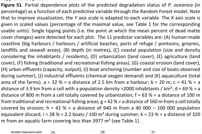
Figure S1. Partial dependence plots of the predicted degradation status of P. oceanica (in
percentage) as a function of each predictive variable through the Random Forest model. Note that to improve visualization, the Y axis scale is adapted to each variable. The X axis scale is given in scaled values (percentage of the maximal value, see Table 1 for the corresponding usable units). Single tipping points (i.e. the point at which the mean percent of dead matte cover changes) were detected for each plot. The 11 predictor variables are: (A) human-made coastline (big harbours / harbours / artificial beaches, ports of refuge / pontoons, groynes, landfills and seawall areas), (B) depth (in metres), (C) coastal population (size and density considering the inhabitants / residents), (D) urbanization (land cover), (E) agriculture (land cover), (F) fishing (traditional and recreational fishing areas), (G) coastal erosion (land cover), (H) urban effluents (capacity, output), (I) boat anchoring (number and size of boats observed during summer), (J) industrial effluents (chemical oxygen demand) and (K) aquaculture (total area of the farms). a = 32 % = a distance of 2.5 km from a harbour; b = 20 m; c = 41 % = a distance of 3.9 km from a cell with a population density >2000 inhabitants / km²; d = 69 % = a distance of 800 m from a cell totally covered by urbanization; f = 63 % = a distance of 100 m from traditional and recreational fishing areas; g = 42 % = a distance of 560 m from a cell totally covered by erosion; h = 42 % = a distance of 940 m from a 40 000 – 100 000 population equivalent discard; i = 28 % = 2.2 boats / 100 m² during summer; k = 23 % = a distance of 320 m from an aquatic farm covering less than 3977 m² (see Table 1).