HAL Id: hal-00787890
https://hal-enpc.archives-ouvertes.fr/hal-00787890
Submitted on 17 Apr 2018
HAL is a multi-disciplinary open access
archive for the deposit and dissemination of
sci-entific research documents, whether they are
pub-lished or not. The documents may come from
teaching and research institutions in France or
abroad, or from public or private research centers.
L’archive ouverte pluridisciplinaire HAL, est
destinée au dépôt et à la diffusion de documents
scientifiques de niveau recherche, publiés ou non,
émanant des établissements d’enseignement et de
recherche français ou étrangers, des laboratoires
publics ou privés.
Do overarching mitigation objectives dominate
transport-specific targets in the EU?
Frédéric Ghersi, Simon Mcdonnell, Olivier Sassi
To cite this version:
Frédéric Ghersi, Simon Mcdonnell, Olivier Sassi.
Do overarching mitigation objectives
dom-inate transport-specific targets in the EU?.
Energy Policy, Elsevier, 2013, 55 (3), pp.3-15.
�10.1016/j.enpol.2012.11.048�. �hal-00787890�
Do overarching mitigation objectives dominate transport-specific
targets in the EU?
Frédéric Ghersia,b Simon McDonnellc Olivier Sassia
a CNRS, CIRED, 45 bis, avenue de la Belle Gabrielle, 94736 Nogent sur Marne CEDEX, France.
b Corresponding author. Email: [email protected]. Phone: +33 1 43 94 73 73. Fax: +33 1 43 94 73 70.
c Office of Policy Research, City University of New York (CUNY), 555 West 57th Street, New York, NY 10019.
Abstract
This research investigates if the stringent 2020 and 2050 overarching CO2 mitigation objectives set out by the European Union dominate its 2010 to 2020 targets specific to the transportation arena, specifi-cally its biofuel penetration objectives and gram CO2 per kilometre emission caps. Using a dynamic re-cursive general equilibrium model, IMACLIM-R, we demonstrate that these overarching targets do not dominate the interim transportation targets when the carbon policy triggering compliance with the mit-igation objectives boils down to the theoretical least-cost option of uniform carbon pricing. Ground transportation is confirmed as quite insensitive to high carbon prices, even when such prices are ap-plied over a long term. It is tempting to conclude that pursuing the mitigatio n objectives specific to transportation will impose unnecessary costs. However, because of the second best conditions prevail-ing in actual economies, and of the risk of lock-in in carbon intensive trajectories, we conclude with the urgent need for some ambitious transport-specific policy design research agenda.
Keywords
Acknowledgments
The authors gratefully acknowledge funding by the European Commission under the TranSust.Scan Pro-ject. A. Vogt-Schilb, CIRED, provided useful comments on a preliminary version and precious support at the time of revision. Two anonymous reviewers significantly helped to improve the paper through their remarks and suggestions. The final document is the sole responsibility of the autho rs.
Introduction
The European Union developed two important and related strategies concerning transportation and sustainability in 2001. The first, the White Paper on Transport, investigated the trends in transport for the coming decade and proposed a number of policy packages (CEC, 2001a). The second, the Sustaina-ble Development Strategy (SDS), articulated, for the first time, an integrated EU policy on sustainability (CEC, 2001b). Recent reviews of both documents reaffirmed and extended the commitments o f Europe-an policymakers in these areas. The White Paper on TrEurope-ansport was central to EuropeEurope-an policymaking in this area for the period up to 2010 and received considerable attention from policymakers and re-searchers alike. It has recently been replaced by a new strategy for the period up to 2020 (CEC, 2011a). However, relatively little academic focus has centred on the potential impacts of the SDS on transporta-tion trends in the European Union. Its overriding environmental objective is to cap the increase in glob-al temperature rise to 2°C above pre-industriglob-al levels by the end of this century. In order to achieve this goal, the European Union (EU) has committed itself to stringent interim targets in carbon dioxide (CO2) emissions reductions by 2020 and 2050 respectively. The target is to reduce EU emissions by 20% com-pared to 1990 levels in the absence of any international agreement by 2020 and by 60 to 80% by 2050 (CEU, 2007). This 2050 target was subsequently raised to an 80 to 95% reduction objective in lat e 2009 through a European Council stated objective within the context of a broader international agreement (DGE, 2011). More recently, the European Commission adopted its “Energy Roadmap 2050” as a basis for developing a long-term European energy use framework that also enshrines the 80-95% target (CEC, 2011b). It is clear that the pursuit and achievement of these long term targets will, almost by necessity, impact on future trends in European transportation.
In this paper, we investigate the impact of these overarching carbon constraints on the more focused short-term transportation objectives outlined in the SDS. To do this, we project the state and trends of European transportation up to 2050 in a business-as-usual or reference scenario, and compare it to an ambitious carbon-pricing scenario that proxies for the 2020 and 2050 emissions targets, at least at their pre-2009 levels.1 The reference and carbon-constrained scenarios are projections of the global dynamic recursive computable general equilibrium model IMACLIM-R. The model has specifically been
devel-oped by CIRED to guarantee a full consistency between macroeconomic and energy balances. Our pur-pose is to develop the above scenarios with the aim of exploring whether reaching both the interim 20% and the long-term 60%-80% reduction in CO2 emissions by 2020 and 2050 through standard carbon pricing necessarily ‘dominates’, i.e. implies compliance with, other targets specifically related to the transport sphere outlined in the SDS—and develop a better understanding as to why it does or does not.
The outline of the paper is as follows: section 1 presents some key transportation trends in the Europe-an Union as it stEurope-ands, it also outlines some of the problems associated with trEurope-ansport, Europe-and investigates some of the key Europe-wide policy responses developed by policymakers. Section 2 briefly reviews the SDS, paying particular attention to its role in relation to transport. Section 3 presents an overview of the IMACLIM-R model and reports key assumptions and general results of the baseline and policy pro-jections. Section 4 focuses on transport and tests the hypothesis outlined above. Finally, section 5 con-cludes with some policy observations.
I. Transportation trends in the European Union
The growth in demand for road transportation in Europe has been rapid in recent decades. European policymakers turned towards analyzing and mitigating the negative impacts of these trends with the publication of the first White Paper on transportation in 1992. But by 2001, the numbe r of cars in the EU had trebled over 1970 levels to almost 175 million and continued to grow by about 3 million cars a year at the turn of the century (CEC, 2001a). In tandem with this, personal mobility on the continent doubled (CEC, 2006) and increased by another 7% in the period up to 2008 (CEC, 2011c). As a result, between 1995 and 2004 road transportation grew by 19% for passenger cars and by 35% for freight movements (measured by passenger-kilometres and tonne-kilometres respectively), continuing a long seen trend. Only with the economic crisis, beginning in 2008, did these trends slow (CEC, 2011c). The impact on Europe’s oil consumption and emissions of greenhouse gases is significant. Transport counts for over 30% of final energy consumption in the EU. By 2006 the road transportation sector ac-counted for 44% of total freight transport (tonne kilometres) and almost 85% of total passenger transport (passenger kilometres) (CEC, 2006). The White Paper Midterm Review (CEC, 2006) notes that the private car accounts for three-quarters of passenger transport while transport by bus and coach combined accounts for less than 10% (these latter modes have grown by a modest 5% over the last decade). As a result of such trends, private cars account for half of ener gy consumed by transport (EEA, 2012). Emissions from domestic transport contributed 21% of all CO2 emissions in Europe—one of the fastest-growing sectors; such emissions grew by 23% over the period 1990 to 2010.2 With road trans-portation heavily dependent on oil (it accounted for 67% of final European demand for oil in 2006 and
by 2008, over 95% of energy use in road transportation was made up of gasoline and diesel (CEC, 2011c)), it alone accounted for almost 85% of CO2 emissions from transport in 2006 (CEC, 2006). These trends have not changed markedly in the interim despite the economic crisis since 2008. The y raised environmental concerns that, coupled with increased concerns about security of energy and institu-tional changes within the EU, have moved transportation towards the centre of the European policy agenda over the last two decades.
The European Commission has long recognised the economic costs of excessive growth in road transport demand (cf. e.g. CEC, 1992; CEC, 1993). It often results in congestion because of the public good nature of road space (Sterner, 2003). But the costs of road transport are not restricted to users of the infrastructure. Indeed, the external costs of road traffic congestion,3 were projected to more than double from 0.5% of EU gross domestic product (GDP) in 2001 by the end of the decade (CEC, 2001a). The recently published White Paper (CEC, 2011a; CEC, 2011c) estimated that congestion costs would reach €200 billion per annum by 2050. The additional costs of road transportation also include acci-dents, road damage externalities and environmental costs. The latter costs consist of regional environ-mental effects (including barrier effects imposed by transportation infrastructure,4 acidification and noise) and air pollution (with both local and global impacts). This point is especially relevant given the increase in transport-related greenhouse gases (GHG) emissions and previously stated broader Europe-an commitments to the Kyoto Protocol Europe-and other initiatives to reduce GHG emissi ons, exemplified by programs such as the European Union Emissions Trading Scheme. Partly as a result of increasing emis-sions from road transport sources (up by 30% since 1990; CEC, 2007), many countries are now strug-gling to meet their commitments to comply with agreed Kyoto Protocol limits.5
Consequently, the focus of European policymakers in the area of transportation has widened from a primarily economic analysis, as per the first White Paper of 1992 (CEC, 1992), to encompass the other two spheres of sustainability, namely the environmental and social areas. This has been mirrored in the development of the 2001 White Paper (CEC, 2001a). This strategy , covering the period up to 2010 (with an update in 2006 that extended analysis to 2020),6 outlined a number of key objectives for transporta-tion in Europe such as providing high levels of mobility to people and businesses while protecting pas-senger safety, energy security, sustainability and efficiency(CEC, 2006).
While longer term objectives aimed at balancing these competing needs were referred to in the 2001 White Paper, specific long-term policy outcomes were beyond its scope. Accordingly, in 2008, the Commission proposed a strategy for greening transportation. The subsequent White Paper, launched in 2011 (CEC, 2011a), attempts to set out a roadmap for a single transportation area and recognises the need for analyses of longer term transportation trends and proposed goals over a time frame of 20 -40 years (CEC, 2007). Specifically, it refers to the need to reduce greenhouse gas emissions by at least 60% by 2050 with respect to 1990 levels. Without any action, it projects that CO2 emissions will be one third
higher by that time. Consequently, while the inter-relations between transport and other areas in the economic, environmental and social spheres were alluded to, it is only with the most recent white pa-per that they have begun to be analysed together. For a broader overview of European polic ymaker’s goals in regard to longer-term climate change objectives, we can continue to look towards the SDS (CEC, 2001b).
II. The European Union Sustainable Development Strategy
The initial move towards sustainability in policymaking was the foundation and reporting of the World Commission on Environment and Development—the ‘Brundtland Commission’—in 1987 (UN, 1987). Its definition of sustainability—development meeting the needs of the present without compromising the ability of future generations to meet their own needs—is the most frequently cited one. The 1992 Unit-ed Nations Conference on Environment and Development (UNCED) in Rio de Janeiro, Brazil followUnit-ed. It adopted Agenda 21 (the Rio Declaration). By 2001, European leaders also moved to incorporate sus-tainability into the policymaking lexicon. The European Council present ed A Sustainable Europe for a
Better World: A European Strategy for Sustainable Development (CEC, 2001b). First proposed by the
European Commission, it was adopted as the Sustainable Development Strategy (SDS) in 2001.
Initially a broad statement of intent recognising the relationship between long-term economic growth, social cohesion and environmental protection, the strategy was re -launched in 2006 and further re-viewed in 2009 with specific targets updated and developed.7 The renewed strategy aims to implement a coherent longterm strategy and places emphasis both on immediate problems and also on longer -term objectives. The 2009 review focused on ‘mainstreaming’ sustainable development policies into European policymaking and reiterated the updated goals. The review outlines an absolute target of a 15-30% reduction over 1990 CO2 emission levels by 2020;8 this was subsequently articulated by the Commission as a commitment to reduce emissions by 20% by 2020 in the absence of an international agreement on climate change and 30% with one (CEC, 2008). It also defines the 2°C cap on temperature increases over the century compared to pre-industrial levels. The European Council subsequently trans-lated this into an EU objective of 60% to 80% reduction over 1990 leve ls in 2050 (CEU, 2007). The over-all transportation objective is identified as ensuring that transport systems meet society’s economic, social and environmental needs whilst minimising negative transport -related externalities in these are-as. Transportation targets include decoupling economic growth and transport demand, reducing GHG emissions from transport, modal shift towards more efficient modes, and reducing CO2 emission from new light duty vehicles. Initially set at 120 grams of CO2 per kilometre (gCO2/km) by 2012, the objective was redefined in 2009 (regulation No 443/2009) to be 130gCO2/km. The former target was postponed to 2015; an additional goal of 95gCO2/km by 2020 was stated.9
Despite the flexibility in target formulation and development shown in the SDS process, neither it nor the various transport white papers explore how the achievement of the long -term climate change goal will impact on shorter-term transportation targets. While some targets have broad interpretations so as to be able to incorporate the impacts of the long-term targets, others are more specific. This juxtaposi-tion between the short-term sub-targets in EU policy-making related to transportajuxtaposi-tion and the long-term climate change objectives develops into an interesting story for re searchers. This is especially true given that the EU proposes to embark on a process that will indirectly address these interactions more closely. The 2011 White Paper (CEC, 2011a) adopts some 40 initiatives for the next decade with the aim of building a competitive and efficient transport system while dramatically reducing Europe’s depend-ence on imported energy and cutting transport carbon emissions 60% below their 1990 level by 2050. But little mention is made of the shorter-term implications of meeting these longer-term targets. We investigate this relationship and, in doing so, complement the recent White Paper by developing a poli-cy scenario aimed at exploring the impact of achieving the ultimate climate change aims of both a 20% and a 60-80% reduction in CO2 emissions by 2020 and 2050 respectively on transport sub -targets.
III. Scenario Development
The baseline and the policy scenario that allow us to test our research hypothesis are projections of the IMACLIM-R model; both the model and the scenario assumptions are outlined below.
III.1. The IMACLIM-R Model
IMACLIM-R is a hybrid recursive general equilibrium model of the world economy divided into 12 re-gions and 12 sectors (Sassi et al., 2009). The model is solved in sequential yearly time steps. The base year of the model (2001) is built on the balanced Social Accounting Matrix (SAM) of the world economy developed by the Global Trade Analysis Programme (GTAP-6 database), modified to accommodate the 2001 International Energy Agency (IEA) energy balances. This data treatment effort is done to base the IMACLIM-R model on a set of hybrid energy-economy matrixes where the production and consumption volumes of the energy sectors are expressed in genuine energy units (million tons-of-oil equivalent, MTOE).
As a general equilibrium model, IMACLIM-R provides a consistent macroeconomic framework to assess the energy-economy relationships by means of clearing factor and goods markets. Rooted in its hybrid calibration, the modelling architecture specifically aims at an easy incorporation of technological infor-mation coming from bottom-up models and experts’ judgements into the projected economic trajecto-ries: physical variables that explicitly characterise equipment, infrastructure and technologies ( e.g. the
efficiency of cars, the intensity of production in transport measured in tonne -kilometres, etc.) allow rigorously modelling how final demand and technical systems are transformed by economic incentives . The economy is thus defined both in money-metric terms and in physical quantities, with the two di-mensions linked by a price vector. This dual vision is designed to guarantee a realistic technical back-ground to the projected economy or, conversely, a realistic economic backback-ground to any projected technical system.
To fully exploit the potential of this dual representation requires abandoning the use of conventional aggregate production functions that, after Berndt and Wood (1975) and Jorgenson (1981), were admit-ted to mimic the set of available aggregate production techniques and thus the technical constraints impinging on an economy. Indeed, it is arguably impossible to find mathematical functions flexible enough to encompass different scenarios of structural changes resulting from the interplay between consumption styles, technologies and localisation patterns (Hourcade, 1993), for small as well as for large departures from the reference equilibrium. In IMACLIM-R, the absence of formal production func-tions is compensated for by a recursive structure that allows for a systematic exchange of information between:
An annual static equilibrium module with Leontief production functions (fixed equipment stocks and intensities of intermediary inputs, especially labour and energy )—but flexible utilisation rates. Solving this equilibrium at some year t provides a snapshot of the economy: information about rela-tive prices, output levels, physical flows and profit rates for each sector and allocation of invest-ments among sectors.
Dynamic modules, including demography, capital dynamics and sector-specific reduced forms of technology-rich models, most of which assess the reactions of technical systems to the previous static equilibria. These reactions are then reintroduced into the static module in the form of updat-ed input-output coefficients to calculate year t+1 equilibrium.
Between two equilibria, technical choices are fully flexible for new capital only : input-output coeffi-cients and labour productivity indexes are modified at the margin, to account for the fixed techniques embodied in existing equipment and resulting from past technical choices. This general ‘putty-clay’ as-sumption is critical to representing the inertia in technical systems and the perverse effect of volatility in economic signals.
IMACLIM-R thus generates economic trajectories by solving successive yearly static equilibria of the economy interlinked through dynamic modules. Within the static equilibrium, in each region, the de-mand for each good is derived from household consumption, government consumption, investment and intermediate uses from the production sectors. Supply is derived from domestic production or imports, as all goods and services are traded on world markets. Domestic and international markets for all
goods—excluding labour—are cleared by a unique set of relative prices that depend on the demand and supply behaviours of representative agents. The calculation of this equilibrium determines relative prices, wages, labour, quantities of goods and services, and value flows.
In this framework, the main exogenous drivers of economic growth are population and labour produc-tivity dynamics. However, international trade, particularly that of energy commodities, and imperfect markets for both labour (wage curve) and capital (constrained capital flows, varying utilisati on rates of productive capacities) can significantly impact on economic growth.
In the IMACLIM-R model transportation activities are typically modelled as complex technical systems constrained by the consistent general macroeconomic framework (cf. Appendix):
First, the transportation demand described in the static equilibrium module allows for the repre-sentation of stylised facts, such as rebound effects associated with energy efficiency improvement or the demand induction by infrastructure that impact both total mobility and the underlying modal breakdown. To that end, the mobility of households is defined as an aggregate of 4 imperfectly sub-stitutable travelling modes (air travel, public terrestrial modes, personal cars and non -motorised modes). It is one of the elements of the utility function of the representative household of each re-gion. In addition to their budget constraint, households are subject to a travelling -time constraint. Last but not least, a ‘travelling time efficiency’ (average distance co vered in an hour of time) factor for each mode is described as an increasing function of public investment in the infrastructure ded-icated to this mode. As for productive sectors, transport consumption, an intermediate input, de-pends on the crossing of specific input-output coefficients (reflecting each sector’s transportation intensity) and the level of activity in each economic sector.
Second, the transportation dynamic module allows for the altering of technical constraints that hinge on transportation demand formation in the static equilibrium: the module keeps track of and marginally modifies the fleet composition and energy efficiency of personal cars, the transport in-tensity of economic activity and, last but not least, the particulars of infrastructu re policies. The total time dedicated by households to mobility evolves in tandem with total population. The motor-isation rate is a function of per capita disposable income, according to an income-elasticity that quad-ratically declines as it increases, up to a 700 vehicles per 1000 inhabitants asymptote meant to translate a saturation effect.
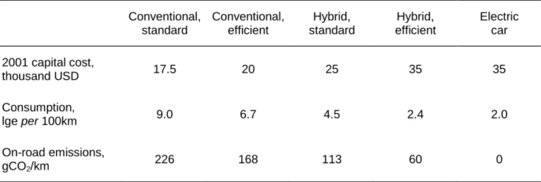
On the technology side,10 evolution of the mean energy intensity of the automobile fleet is related to final energy prices through a representation of households’ equ ipment choices among 5 representative car technologies: standard and efficient conventional cars, standard and efficient hybrid cars and elec-tric cars. Each technology is characterised by a capital cost and an energy efficiency expressed in litres of gasoline equivalent (lge) per 100 kilometres. Table 1 sums up the technology characteristics for
Eu-rope.11 Each year, car sales induced by the evolution of the equipment rate and retirement of the oldest vintage are split between the 5 technologies according to their lifecycle costs (LCC) over an undifferen-tiated 15-year usage and for the current region-specific average annual mileages. The split is dictated by a multinomial logit function to account for heterogeneous preferences and the diversity of car uses, based on a 13% private discount rate. The capital costs of each technology evolve according to a 10% learning curve,12 while the energy intensities are constant over time: the efficient versions of the con-ventional and hybrid technologies amount to efficiency asymptotes at the projecting horizon (2050); the endogenous shifts of their rates of penetration allow covering a continuum of (average) fuel effi-ciencies and g/km emissions for both technologies between the higher bound s defined by their stand-ard versions and the lower bounds defined by their efficient versions.13
Conventional, standard Conventional, efficient Hybrid, standard Hybrid, efficient Electric car 2001 capital cost, thousand USD 17.5 20 25 35 35 Consumption, lge per 100km 9.0 6.7 4.5 2.4 2.0 On-road emissions, gCO2/km 226 168 113 60 0
Table 1. European car technologies parameters
Various investment policies can be tested for their impact on average modal speeds. Throughout this paper and due to brevity concerns, however, we stick to the conservative assumption that the building of transportation infrastructure follows the evolution of modal mobility.
Road and rail freight and public passenger transportation are aggregated in one productive s ector. The evolution of this sector’s energy input coefficients therefore accounts for both energy efficiency gains and shifts between road and rail modes. This evolution is triggered by final energy price variations, based on a compact reaction function calibrated on bottom-up information from the POLES energy sec-tor model (Criqui, 2001). The evolution of the freight content of economic growth, which is represented by the transportation input-output coefficients of all the productive sectors in the economy , is an exog-enous scenario variable in this paper. However, we note that it is indeed debatable how energy prices affect a firm’s choice of localisation and production management and these parameters are likely to play a central role in cost-effective mitigation policies (Crassous et al., 2006).
Finally, fuels are produced by a petroleum products sector, undifferentiated between gasoline and die-sel. Biofuels and coal-to-liquid (CTL) fuels progressively enter the fuel mix. Biofuel penetration follows a set of worldwide supply curves provided by the IEA (IEA, 2006, pp. 283 and 288) for bio -ethanol and bio-diesel production, that are transposed as functions of the production price of conventional fuels
augmented by the carbon tax differential (the difference between the carbon tax levied on convention-al fuels and that levied on each biofuel).14 CTL penetration is based on a microeconomic representation of investment behaviour, taking into account the dynamics of oil prices and some constraint on growth also derived from IEA analysis (IEA, 2008).15
III.2. The baseline or ‘reference’ (REF) scenario
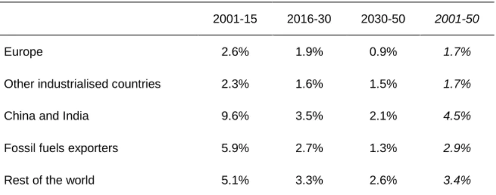
The baseline or ‘reference’ (REF) scenario depicts business-as-usual economic growth in the absence of any carbon constraint (Table 2). At the world level, it envisages a doubling of real per capita income between 2001 and 2050, and thus corresponds to the lower range of the SRES scenarios (Nakicenovic et
al., 2000), between the A2 and the B2 markers (which multiply per capita income by 1.8 and 2.5
respec-tively). Behind this aggregate picture, regional dynamics differ substantially as they are characterised by a partial catch up between industrialised and developing countries ( cf. e.g. Barro and Sala-i-Martin, 1991, 1992; Quah, 1996):16
Europe and the other industrialised countries (OIC) suffer from a demographic slowdown that is unequally compensated by sustained gains of labour productivity. Compared to OIC, Europe is as-sumed to benefit from higher labour productivity improvements over the first three deca des (the catch-up hypothesis), which results into higher growth.
China and India have their extremely high current growth rates reduced, as (i) their labour produc-tivity improvements increase to a peak, (ii) their demography stabilises, and (iii) rapidly increasing energy prices hamper their relatively energy-intensive economic activity.
Fossil fuels exporters (FFE) suffer from both stabilising demographics and a relatively low gain in labour productivity, that are imperfectly compensated by the rents they extract from increasingly tense energy markets.
In the rest of the world (ROW), increases in labour productivity slowly take over the sheer impact of demographics as the latter effect slows down.
2001-15 2016-30 2030-50 2001-50
Europe 2.6% 1.9% 0.9% 1.7%
Other industrialised countries 2.3% 1.6% 1.5% 1.7%
China and India 9.6% 3.5% 2.1% 4.5%
Fossil fuels exporters 5.9% 2.7% 1.3% 2.9%
Rest of the world 5.1% 3.3% 2.6% 3.4%
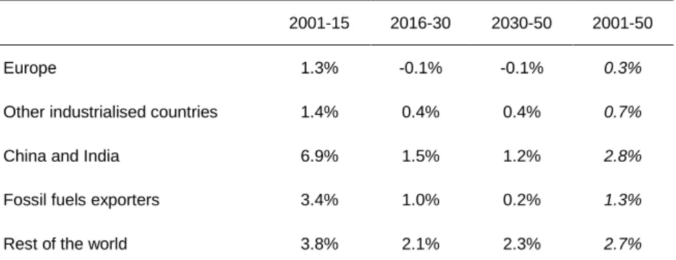
2001-15 2016-30 2030-50 2001-50
Europe 1.3% -0.1% -0.1% 0.3%
Other industrialised countries 1.4% 0.4% 0.4% 0.7%
China and India 6.9% 1.5% 1.2% 2.8%
Fossil fuels exporters 3.4% 1.0% 0.2% 1.3%
Rest of the world 3.8% 2.1% 2.3% 2.7%
Table 3. Average annual growth of CO
2emissions, REF scenario
Turning to environmental performance, the comparison of Table 2 and Table 3 reveals a significant de-coupling of growth and CO2 emissions. In the absence of carbon constraint this is mainly due to two major determinants:
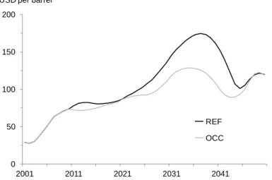
First, the physical constraints that limit the evolution of fossil fuel supply lead to a general increase of fossil energy prices along the projection. The price of coal on international markets experiences a 73% increase between 2001 and 2050, and the price of natural gas increases by almost 160% over the same period. The price of oil displays the most dramatic increase (cf. Figure 4 below): starting from $29 per barrel (hereafter /bbl) in 2001,17 it peaks at a $175/bbl maximum in 2037, when the continuingly growing global demand comes closest to the ever slower developing global production capacity.18 After 2037 it gradually decreases, reaching $120/bbl in 2050, as energy-efficient tech-nologies enter the markets and alternative liquid fuel production (mainly second generation biofu-els and synthetic fubiofu-els from coal-to-liquid production) develops. This general increase in fossil fuel prices fosters both the penetration of carbon-free energy sources (renewable and nuclear) into the primary energy mix, and the diffusion of energy-efficient equipment, which reduce the energy in-tensity of economic growth. Higher energy prices also induce structural changes in the econo mies in favour of the less energy-intensive activities.
Second, the general increase in wealth is endogenously associated with a dematerialisation of growth: as per capita income increases, economies move from a base of (energy-intensive) heavy industries to one in which services dominate. Dematerialisation is projected for the industrialised world, to a lesser extent for China and India, and in a subtly different way for fossil fuels exporters as well (a significant part of their dematerialisation occurs t hrough the increasing rents they draw from energy markets). It is much weaker for the rest of the world due to the ‘mimetic development’ assumption backing the REF scenario: developing countries are assumed to pursue the same life-style as industrialised countries as their per capita income rises: they increase the size of their homes and buy more home equipment, switch to personal cars as their dominant transportation mode, etc. —these development trends are explicitly modelled in IMACLIM -R.
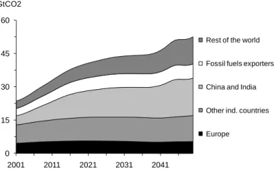
For Europe, the resulting carbon emissions profile rises to a +19% (over its 1990 level) peak in 2020, then gradually decreases to reach +13% in 2050 (Figure 1).
Figure 1. CO
2emissions in the REF scenario
III.3. The ‘overarching carbon constraint’ scenario
The ‘overarching carbon constraint’ (OCC) policy scenario departs from the REF scenario in that it en-visages the implementation of carbon prices on a global scale from 2011 on, based on:
The central assumption that Europe aims at CO2 emissions both at least 20% below their 1990 level in 2020, and with a long term objective at the lower range of its 60 to 80% target. Compliance with these constraints is attained through the simplest instrument of a uniform pricing of carbon (a generalised carbon tax).
The complementary hypothesis that the world outside Europe follows the European lead by apply-ing the European price signals downgraded by 20% for the OIC, and 80% for all other regions. With our focus on Europe and its transportation activities, the latter set of assumptions i s not essential to our demonstration. It is only proposed as a more plausible option than unilateral action by Europe, which would cause strong distortions on international markets given the levels of carbon prices implied by the constraints.
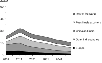
Figure 2 plots one European emission path compatible with these objectives, and the emissions of the 4 other world regions previously outlined implied by their crudely hypothesised ‘follower behaviour’.19 Global emissions reach a strikingly early 32,8 billion tonnes of CO2 (hereafter GtCO2) peak in 2012, then decrease down to 15,9 GtCO2 in 2050. European emissions, on which we focus, reach an even more early 2010 peak at 12% over their 1990 level; they then decrease to 22% below this level in 2020, and end up at 65% below this level in 2050.
0 15 30 45 60 2001 2011 2021 2031 2041 GtCO2
Rest of the world
Fossil fuels exporters
China and India
Other ind. countries
Figure 2. CO
2emissions in the OCC scenario
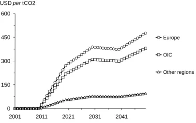
The price signals required to achieve the challenging European emission reduction objectives, together with their downgraded values prevailing in other regions of the world, are presented in Figure 3. The European trajectory can be divided in three characteristic periods:
Between 2011 and 2030 the price of carbon increases very fast (+27.2 year 2001 US dollars per tonne of CO2—hereafter $/tCO2—per year) to reach $272/tCO2 in 2020, then fast (+$11.6/tCO2 per
year) to $388/tCO2in 2030. The particular shape of this signal is related to a demanding 2020 re-duction objective (corresponding to a 33% decrease from REF emissions) that has to circumvent the high inertia of capital stocks and the myopic behaviour of economic agents.
Between 2030 and 2040 the price of carbon slightly decreases, as the technical change induced by early and ambitious climate policies diffuses, developing some emission reduction potentials at lower costs.
After 2040, the looming stringent 2050 target requires additional reductions that are more expen-sive and carbon prices again experience a fast increase (+$10.3/tCO2 per year).
0 15 30 45 60 2001 2011 2021 2031 2041 GtCO2
Rest of the world
Fossil fuels exporters
China and India
Other ind. countries
Figure 3. CO
2price trajectories in the OCC scenario
20The emission reductions triggered by those prices are related to major changes in the European energy sector. They are obtained, on the demand side, through the rapid diffusion of very -low-emission equipment in the building, transportation (see below), and industrial sectors, that allow a 59% re duc-tion in the primary energy intensity of European GDP between 2001 and 2050 —while in 2020 the re-duction is already of 19% compared to 2001. On the supply side, low -carbon and carbon-free energy technologies, such as renewables, third generation nuclear p ower, and carbon capture and storage spread widely to allow a 60% cut in the CO2 intensity of total primary energy supply between 2001 and 2050—the cut is 35% in 2020 compared to 2001.
2001-15 2016-30 2030-50 2001-50 Europe 2.4% (-0.2) 1.8% (-0.1) 1.1% (+0.1) 1.6% (-0.0)
Other industrialised countries 2.1%
(-0.2) 1.5% (-0.0) 1.6% (+0.1) 1.7% (-0.0)
China and India 9.1%
(-0.4) 3.3% (-0.1) 2.3% (+0.1) 4.4% (-0.1)
Fossil fuels exporters 4.8%
(-1.0) 2.6% (-0.1) 1.7% (+0.4) 2.8% (-0.1)
Rest of the world 4.9%
(-0.1) 3.3% (-0.0) 2.6% (-0.0) 3.4% (-0.1)
Table 4. Average annual growth of real GDP, OCC scenario
In brackets: percentage point deviation from the REF scenario (cf. Table 2).
The general macroeconomic consequences of such major mutations of the energy systems are not as dramatic as one might expect—although it must be kept in mind that a GDP growing 1.7% a year will be 5% above one growing 1.6% a year after 50 years. They depend to some extent on the characteristics of each region, but, generally speaking, economies bear the brunt of the constraint in the shorter run (Table 4Erreur ! Source du renvoi introuvable.Erreur ! Source du renvoi introuvable.), when they are
0 150 300 450 600 2001 2011 2021 2031 2041
USD per tCO2
Europe
OIC
hampered by the inertia of their energy systems; in the longer run, when the necessary adjustments have taken place, growth tends back towards its REF levels, and even overshoots it in some regions. The possibility of overshooting the baseline in such a modelling architecture as IMACLIM -R is linked to the imperfect foresight assumption it adopts for all economic agents. The REF scenario is characterised by huge tensions on the oil markets that are not well anticipated. The climate policy gives a strong signal towards decarbonisation early enough in the trajectory to induce additional technical change for energy efficient technologies that does not occur in the baseline because of the lack of an early enough antici-pation of the future tensions on oil markets. Economies thus can use more efficient technologies in the OCC scenario for a cost lower than in the REF scenario. It is indeed the case for Europe, which, after a loss of 0.2 points of annual growth between 2001 and 2015, decreasing to 0.1 point between 2016 and 2030, experiences a gain of 0.2 points of annual growt h in the 20 last years of projection.
The impact on the other industrialised countries is smaller because of both a lower carbon price, and larger low-cost reduction potentials (esp. in the US). India and China are particularly hit, as they com-bine the impacts of a carbon constraint—much downgraded but still significant for their developing carbon-intensive economies—with that of a diminution of international trade mechanically caused by a lower global growth. In a similar way but on different markets, foss il fuel exporters are strongly hit be-fore 2030, as they see both their export volumes greatly reduced, and the consequently much lower tensions on the oil and gas markets decrease their rents ( cf. the OCC vs. REF price of oil on international markets, Figure 4 below).
Figure 4. International price of oil in the REF and OCC scenarios
21Still, the OCC scenario as it stands is somewhat conservative as it does not h ypothesise climate policy-induced changes in lifestyles, location and urbanisation choices. It would be reasonable to assume that climate policies could be complemented by other public policies to induce such behavioural changes
0 50 100 150 200 2001 2011 2021 2031 2041
USD per barrel
REF OCC
(that are not very reactive to carbon prices) in a consistent way with the climate objective. The cost of stabilisation would probably be reduced with such a policy package (cf. e.g. Gusdorf et al., 2008).
IV. European road transportation: from current trends to a carbon
constrained European Union
Let us now turn to the analysis of how the 2020 and 2050 OCCs impact the CO2 emissions from ground transportation in Europe. To systematise this analysis we will successively report mobility, energy con-sumption (backed by an analysis of the private car fleet), and CO2 emissions for motorised ground transport.
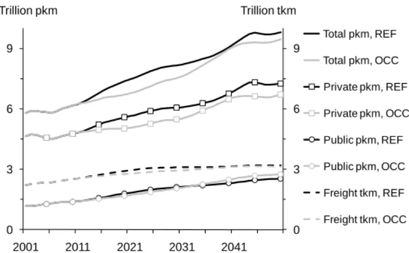
Aggregate motorised ground passenger mobility (i.e. the sum of private car, bus and rail passenger mo-bility), measured in passenger-kilometres (pkm), appears quite resistant to the high carbon prices pre-vailing in the OCC scenario (Figure 5, left-hand axis). Its impact is reminiscent of the GDP trends: a slight decrease is observed in the short- to medium-term, then some catching-up occurs beyond 2030, alt-hough pkm stay below their REF value. Within this aggregate evolution the split between public and private transportation is also relatively unchanged. It only slightly evolves in the favour of the former modes, which end up above their REF level by 2050 as they naturally benefit from a much lower carbon intensity per pkm. Notwithstanding, these results fundamentally confirm the oft -reported finding (see
e.g. Espey, 1998, or Goodwin et al., 2004, for a survey), somewhat disturbing for policy -makers, that
even high carbon prices have only a marginal impact on mobility in both quantitative and qualitative terms.
Figure 5. European motorised ground mobility
The evolution of freight tonnes-kilometres (tkm) follows a pattern similar to that of GDP, as freight transport highly depends on the overall level of activity. However, the impact of OCC on freight activity
0 3 6 9 0 3 6 9 2001 2011 2021 2031 2041 Trillion tkm Trillion pkm Total pkm, REF Total pkm, OCC Private pkm, REF Private pkm, OCC Public pkm, REF Public pkm, OCC Freight tkm, REF Freight tkm, OCC
ends up being stronger (-2.0% tkm in 2050 compared to REF) than its impact on GDP ( -1.1%). This re-flects the impact of the stringent climate policy on the structure of the economy, which turns towards sectors that are less intensive in materials and transportation.
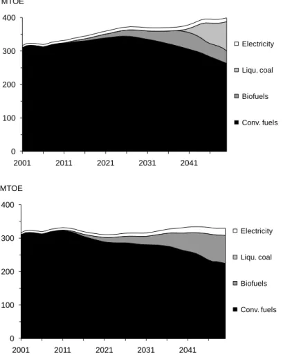
Still, ground motorised mobility appears to be relatively insensitive to high carbon prices in both its passenger and freight dimensions. This result is echoed to some extent in the related energy consump-tion. Measured in million tonnes of oil equivalent (MTOE), consumpt ion declines in the OCC scenario compared with their REF values (Figure 6), but the high carbon prices required by the OCC fail to curb down total energy consumption in absolute terms, and barely achieve its stabilisation. The split be-tween fuels is also only marginally impacted; conventional fuels retain their two -third share of total energy: high carbon prices have the counter-intuitive effect of relaxing the tensions on international oil market, thus moderating the ultimate relative impact of OCC on gaso line prices. In the remaining third, however, the massive development of coal-to-liquid technologies projected in REF is blocked by high carbon prices, in the favour of biofuels, whose 2050 production is 120% higher than in the REF scenario. Although hybrid and electric cars begin to weigh in the total fleet at the end of the projected period (17.3% market share in 2050),22 the share of electricity remains low (6.5% in 2050) as this technology benefits from a high energy efficiency.
Figure 6. End-use energy consumption of ground transportation,
REF (upper graph) vs OCC (lower graph) scenario
To investigate these trends further, we focus on technical changes that alter the energy intensity and fuel mix in the transportation sector.
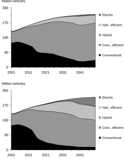
As far as private cars are concerned, the 2001-2050 reduction in energy intensity (MTOE/pkm) shifts from 20% in the REF scenario to 34% in its OCC counterpart. These higher energy efficiency improve-ments are due to market penetration of more efficient conventional cars and hy brid and electric cars (Figure 7). In the OCC scenario high carbon prices act as a signal and the fleet shares of less emitting technologies are boosted. Indeed, the share of non-conventional vehicles in 2030 increases from 10% in the REF scenario to 25% in the OCC scenario. We see further sustained growth in these technologies up to 2050 where they account for 17% of the on-road fleet in the REF scenario and 44% in the OCC sce-nario. 0 100 200 300 400 2001 2011 2021 2031 2041 MTOE Electricity Liqu. coal Biofuels Conv. fuels 0 100 200 300 400 2001 2011 2021 2031 2041 MTOE Electricity Liqu. coal Biofuels Conv. fuels
Figure 7. Share of technologies in the private car fleet,
REF (upper graph) vs OCC (lower graph) scenario
While overall mobility is not affected by the carbon pricing strategy, the composition of the fleet (in terms of fuel choice and efficiency) thus undergoes some significant changes. Interestingly, we do see some catch-up in the REF scenario towards the second half of the time period. This trend occurs be-cause of the increase in oil prices in the 2025-2040 period, which creates its own price signal to con-sumers. However, the massive carbon pricing in the OCC scenario ind uces a stronger shift towards the cleaner technologies (whereas the increases in oil prices are much more moderate due to much lower tensions on oil markets) and prevents a comeback of less efficient technologies that occurs in the REF scenario as tensions on oil market are relaxed by the increasing production of synthetic fuels.
Efficiency improvements are less important in the public transportation sector (freight and passengers) where the high carbon prices of OCC induce a modest 6.9% decrease in energy intensity compared to REF in 2050. This difference is mainly due to potentials for efficiency improvement, that are pictured by IMACLIM-R as high in the current automobile fleet (downsizing, material substitution, engine improve-ments), but more conservatively for trucks and buses, reflecting consensual vs. more debated assump-tions (IEA, 2009). 0 90 180 270 360 2001 2011 2021 2031 2041 Million vehicles Electric Hyb., efficient Hybrid Conv., efficient Conventional 0 90 180 270 360 2001 2011 2021 2031 2041 Million vehicles Electric Hyb., efficient Hybrid Conv., efficient Conventional
Turning to CO2 emissions, we find that ground transportation emissions do not follow the total emis-sions trend constrained by the OCC scenario, at least under our hyp othesis that this trend is achieved through the sole policy instrument of uniform carbon pricing. Reductions in ground transportation emissions under OCC indeed amount to 14% of REF emissions in 2020, 25% in 2050 (Figure 8). These figures are to be compared with the massive overall decreases of 34% and 69% achieved at those target dates, and ultimately tend to prove that transportation stands as an obstacle to stringent stabilisation objectives, at least when these objectives are pursued through carbon pric ing policies only.
Figure 8. Tank-to-wheel CO
2emissions of ground transportation,
REF (upper graph) vs OCC (lower graph) scenario
Finally, we analyse how these results translate in terms of the specific transportation targets set by the EU. The level of detail of IMACLIM-R allows us to test in particular two policy areas of the transport arena that are addressed in the SDS. The first policy area relates to the penetration of biofuels in the market for transport fuel, with targets set for 2010 and 202 0.23 The second relates to average emissions of CO2 per km from the new car fleet, for 2012, 2015 and 2020.24
0 300 600 900 2001 2011 2021 2031 2041 MtCO2
Buses, trucks & rail Passenger cars 0 300 600 900 2001 2011 2021 2031 2041 MtCO2
Buses, trucks & rail Passenger cars
Generally speaking, we find that all the outlined targets are missed in OCC as in REF, and missed by considerable distances (Table 5).
Target Year Objective REF scenario OCC scenario
Share of biofuels (EC 30/2003) 2010 5.75% 0.19% 0.19% Share of biofuels (CEU, 2007) 2020 10% 2.95% 4.02% LDV CO2 emis-sions, bench-test vintage average (SDS target) 2012 120 g/km 134 g/km 127 g/km LDV CO2 emis-sions, bench-test vintage average (EC 443/2009) 2015 120 g/kma 134 g/km 127 g/km LDV CO2 emis-sions, bench-test vintage average 2020 95 g/km 132 g/km 120 g/km
a The target is more precisely defined as 130g/km on average for the total sales of each carmaker (with derogative
provisions for very small producers), complemented by an extra 10g/km reduction from “additional measures”, cf. regula-tion EC 443/2009.
Table 5. Status of transport objectives under the two scenarios
Bench-test vintage averages of the REF and OCC scenarios are systematically estimated 18% below the projected on-road vintage averages (cf. endnote 13)
On biofuel penetration, in 2010 biofuel development spectacularly fails to meet its target, irrespective of the OCC, for the simple reason that the policy scenario does not diverge from the REF trajectory be-fore 2011. in 2020 the OCC scenario starts to make a visible difference, as both the price incentive has developed, and time has elapsed allowing the development of production capacities. Still, the target is far from being reached: biofuels development still only makes up 40% of the target.
The results on the average CO2 efficiency of new cars are more sensitive to the OCC scenario in the short term: as early as 2012 imposing the OCC cuts the 14 g/km compliance gap of REF in half. This higher responsiveness of fuel efficiency to pricing strategies is in part explained by the lesser inertia of mere market share shifts for already existing technologies (more efficient conventional vehicles and hybrid vehicles), compared to the development of industrial biofuel capacities. Still, by 2020 the 37 g/km excess is only cut down to 25 g/km, and the 95 g/km is miss ed by 26%.
These findings point once again at the low reactivity of the transportation sector to carbon policies that are exclusively price-based. Even in an ambitious climate scenario, in which policymakers resort to a stringent pricing of carbon with the aim of fulfilling an overarching reduction objective, there is no guarantee that interim or long term policy targets will be attained for the transportation sector. The biofuel and energy efficiency policy objectives are goals in themselves, which appear to require
addi-tional policy initiatives to be achieved. As a result, based on this evidence, we reject the hypothesis that the presence of such a long-range target will ‘dominate’ specific sectoral objectives.
Conclusion
Our research rejects the hypothesis that even stringent short- and long-term overarching CO2 mitiga-tion targets dominate (i.e. necessary imply compliance with) short-run objectives in the transportamitiga-tion arena. More specifically, our simulations demonstrate that hitting mitigation targets in the lower range of outlined overarching European objectives, i.e. constraining CO2 emissions 22% and 65% below their 1990 level in 2020 and 2050 respectively, through the implementation of uniform economy -wide car-bon prices, does not succeed in triggering significant changes in the transportation sector compatible with outlined 2010 to 2020 biofuels penetration and CO2 intensity targets. Even in the longer term, car-bon prices close to an impressive $500/tCO2 do not succeed in curbing CO2 emissions from ground transportation by more than a modest 25% decrease from their baseline trend . This is a significant step away from the 60% below 1990 levels objective of the 2011 White Paper on Transport.
In policymaking terms it is tempting to jump to the conclusio n that specific targets on transportation activities are superfluous, if anything unduly costly, as they suppose marginal prices higher than those triggering compliance to the overarching objectives. This would indeed echo the theoretical recom-mendation that an overarching constraint as carbon mitigation should not be fragmented in sectoral targets or technology choices (biofuels) following some unavoidably flawed political process, but should rather be enforced by adjusting a uniform price signal that would ‘naturally’ select the cheaper abate-ment opportunities, free of preconceptions.
For at least two reasons this recommendation can be questioned in the case of carbon mitigation. First, it only prevails in first best economic conditions (perfect markets, perfect information, perfect anticipa-tions), whereas addressing the market failures and imperfections of real economies may require ex-tended policy packages. Guivarch and Hallegatte (2011) thus demonstrate that complementing uniform carbon pricing with policies targeting the development of infrastructures, which is otherwise barred by imperfect foresight and split incentives, significantly cuts down the costs of the more ambitious mitiga-tion objectives. Similarly, the carbon-efficiency mandates quesmitiga-tioned in our research might be a rele-vant policy option to circumvent the ‘split incentive’ issues surrounding company cars . They could also be warranted to bridge the gap between the higher private discount rate governing car technology choices (13% in our modelling exercise) and the lower 3% to 5% discount rate commonly thought to apply to an aggregate ‘social welfare’ perspective. Second, even if it were possible to prove that it is economically inefficient to pursue specific transportation objectives up to 205 0, it would not mean that there is no ground to do so for objectives beyond the OCC, both more stringent and more distant in
time: the resilience of CO2 emissions from ground transportation to carbon pricing hints at a lock -in of this activity in carbon intensive trajectories, that might compromise the ability of Europe to aim at tar-gets in the higher range of their 2050 reduction objective, or even beyond, would e.g. some updated alarming information about climate sensitivity warrant it —Vogt-Schilb and al. (2012) demonstrate in-deed how technical inertia can vouch for differentiated carbon prices. This in turn highlights the urgent need for some ambitious transport-specific policy design research agenda.
References
Barro, R. J., Sala-i-Martin, X., 1991. Convergence across states and regions. Brookings Papers of Eco-nomic Activity, 22 (1), 107-182.
Barro, R. J., Sala-i-Martin, X., 1992. Convergence. Journal of Political Economy, 100 (21), 223 -51. Berndt, E., Wood, D., 1975. Technology, prices and the derived demand for energy. Review of Econom-ics and StatistEconom-ics, 57 (3), 259-68.
Bieber, A., Massot, M.-H., Orfeuil, J.-P., 1994. Prospects for daily urban mobility. Transport Reviews, 14 (4), 321-339.
Commission of the European Communities (CEC), 1992. The future development of the common transport policy. A global approach to the construction of a community framework for sustainable mo-bility. Transport White Paper. COM (92) 494 final, 2 December 1992, Bulletin of the European Commu-nities, Supplement 3/93.
Commission of the European Communities (CEC), 1993. Growth, competitiveness, employment: The challenges and ways forward into the 21st century. White Paper. COM (93) 700 final/A and B, 5 Decem-ber 1993. Bulletin of the European Communities, Supplement 6/93.
Commission of the European Communities (CEC), 2001a. European transport policy for 2010: Time to decide. Transport White Paper. COM (2001) 370 final, 12 September 2001.
Commission of the European Communities (CEC), 2001b. A sustainable Europe for a better world: A Eu-ropean Union strategy for sustainable development. COM (2001) 264 final, 15 May 2001.
Commission of the European Communities (CEC), 2002. Towards a global partnership for sustainable development. COM (2002) 82 final, 13 February 2002.
Commission of the European Communities (CEC), 2006. Keep Europe moving. Sustainable mobility for our continent. Mid-term review of the European Commission’s 2001 Transport White Paper. COM (2006) 314 final, 22 June 2006.
Commission of the European Communities (CEC), 2007. Results of the Review of the Community Strate-gy to Reduce CO2 Emissions from Passenger Cars and Light-Commercial Vehicles, COM(2007) 19 final, 7 February 2007:
http://eur-lex.europa.eu/LexUriServ/site/en/com/2007/com2007_0019en01.pdf
Commission of the European Communities (CEC), 2008. 20 20 by 2020 - Europe's Climate Change Op-portunity, COM(2008) 30 final, 23 January 2008:
http://www.energy.eu/directives/com2008_0030en01.pdf
Commission of the European Communities (CEC), 2011a. Roadmap to a single European transport area. Towards a competitive and resource efficient transport system. COM (2011) 144 final, 28 March 2011:
http://ec.europa.eu/transport/strategies/2011_white_paper_en.htm
Commission of the European Communities (CEC), 2011b. Energy roadmap 2050, COM(2011) 885 final, 15 December 2011:
http://eur-lex.europa.eu/LexUriServ/LexUriServ.do?uri=COM:2011:0885:FIN:EN:PDF
Commission of the European Communities (CEC), 2011c. Impact assessment. Accompanying document to the White Paper Roadmap to a single European transport area. Towards a competitive and resource
efficient transport system. SEC (2011) 358 final, 28 March 2011:
http://eur-lex.europa.eu/LexUriServ/LexUriServ.do?uri=SEC:2011:0358:FIN:EN:PDF
Council of the European Union (CEU), 2006. Review of the EU sustainable development strategy (EU SDS). Renewed strategy. Council of the European Union, Brussels, 26th June 2006.
http://register.consilium.europa.eu/pdf/en/06/st10/st10917.en06.pdf (accessed January, 8th, 2012). Council of the European Union (CEU), 2007. Brussels European Council 8/9 March 2007, presidency conclusions. 7224/1/07 Rev 1, 2 May 2007,
http://www.consilium.europa.eu/ueDocs/cms_Data/docs/pressData/en/ec/93135.pdf (accessed Janu-ary 12th, 2012).
Clarke, L., Edmonds, J., Krey, V., Richels, R., Rose, S., Tavoni, M., 2009. International climate policy ar-chitectures: Overview of the EMF 22 international scenarios. Energy Economics, 31, supplement 2, S64-S81.
Crassous, R., Hourcade, J.-C., Sassi, O., 2006. Endogenous structural change and climate targets. Model-ing experiments with IMACLIM-R. The Energy Journal, special issue Endogenous technological change and the economics of the atmospheric stabilization, 259–276.
Criqui, P. (2001), POLES: Prospective Outlook on Long-term Energy Systems, Institut d’économie et de politique de l’énergie, Grenoble, France,
http://www.upmf-grenoble.fr/iepe/textes/POLES8p_01.pdf (accessed January 12th, 2012).
Dargay, J., Gately, D., Sommer, M., 2007. Vehicle ownership and income growth, worldwide: 1960-2030. The Energy Journal, 28, 143-170.
Directorate-General for Energy (DGE), 2011. Energy roadmap 2050 – State of play: Background paper. 3 May 2011,
http://ec.europa.eu/energy/strategies/2011/doc/roadmap_2050/20110503_energy_roadmap_2050_st ate_of_play.pdf (accessed January 12th, 2012).
Espey, M., 1998. Gasoline demand revisited: An international meta-analysis of elasticities. Energy Eco-nomics, 20 (3), 273-95.
European Environment Agency, 2012. Energy Efficiency and Energy Consumption in the Transport Sec-tor (ENER 023). Assessment published April 2012.
http://www.eea.europa.eu/data-and-maps/indicators/energy-efficiency-and-energy-consumption-4/assessment (accessed July 12th, 2012).
Goodwin, P., Dargay, J., Hanly, M., 2004. Elasticities of road traffic and fuel consumption with respect to price and income: A review. Transport Reviews, 24 (3), 275-92.
Guivarch, C., Hallegatte, S., 2011. Existing infrastructure and the 2°C target. A letter. Climatic Change, 109 (3-4), 801–05.
Gusdorf, F., Hallegatte, S., Lahellec, A., 2008. Time and space matter: How urban transitions create ine-quality. Global Environmental Change, 18 (4), 708-19.
Hourcade, J.-C., 1993. Modelling long-run scenarios. Methodology lessons from a prospective study on a low CO2 intensive country. Energy Policy, 21 (3), 309-26.
International Energy Agency (IEA), 2004. Biofuels for transport: An international perspective. OECD/International Energy Agency, Paris, France.
International Energy Agency (IEA), 2006. Energy technology perspectives 2006. OECD/International En-ergy Agency, Paris, France.
International Energy Agency (IEA), 2008. World Energy Outlook . OECD/International Energy Agency, Paris, France.
International Energy Agency (IEA), 2009. Technology roadmap. Electric and plug-in hybrid electric vehi-cles. OECD/International Energy Agency, Paris, France.
Jorgenson, D.W., 1981. Energy prices and productivity growth. Scandinavian Journal of Economics, 83(2), 165–79.
Nakicenovic, N., Alcamo, J., Davis, G., De Vries, B., Fenhann, J., Gaffin, S., Gregory, K., Grübler, A., Jung, T.Y., Kram, T., La Rovere, E.L., Michaelis, L., Mori, S., Morita, T., Pepper, W., Pitcher, H., Price, L., Riahi, K., Roehrl, A., Rogner, H.-H., Sankovski, A., Schlesinger, M., Shukla, P.R., Smith, S., Swart, R., van Rooi-jen, S., Victor, N., Dadi, Z., 2000. IPCC special report on emissions scenarios. Cambridge University Press, Cambridge, United Kingdom and New York, NY, USA.
Quah, D., 1996. Empirics for economic growth and convergence. European Economic Review, 40 (6), 1353-75.
Rozenberg, J., Hallegatte, S., Vogt-Schilb, A., Sassi, O., Guivarch, C., Waisman, H., Hourcade, J. -C., 2010. Climate policies as a hedge against the uncertainty on future oil supply. Climatic Change, Electronic Supplementary Material.
http://www.springerlink.com/content/u45p6385t6xj8711/10584_2010_Article_9868_ESM.html (ac-cessed January 12th, 2012).
Sassi, O., Crassous, R., Hourcade, J.-C., Gitz, V., Waisman, H., Guivarch, C., 2009. IMACLIM-R: A model-ling framework to simulate sustainable development pathways. International Journal of Global Envi-ronmental Issues, 10 (1-2), 5-24:
http://www.imaclim.centre-cired.fr/IMG/pdf/Sassi_et_al_2010_ImaclimR_a_modelling_framework_to_simulate_sustainable_devel opment_pathways.pdf
Schäfer, A., Victor, D., 2000. The future mobility of the world population. Transportation Research Part A: Policy and Practice, 34(3), 171-205.
Sterner, T. (2003) Policy instruments for environmental and natural resource management . Resources for the Future, Washington, D.C.
United Nations (UN), 1987. Report of the world commission on environment and development. United Nations General Assembly Resolution 42/187, 11 December 1987.
Vilhelmson, B., 1999. Daily mobility and the use of time for different activities: The case of Sweden. GeoJournal, 48 (3), 177-185.
Vogt-Schilb, A., Meunier, G., Hallegatte, S., 2012. How inertia and limited potentials affect the timing of sectoral abatements in optimal climate policy. Policy Research Working Paper 6154, The World Bank, Sustainable Development Network, Office of the Chief Economist.
Vogt-Schilb, A., Sassi, O., Cassen, C., Hourcade, J.-C., 2009. Electric vehicles: What economic viability and climate benefits in contrasting futures? CIRED Working Paper,
http://www.centre-cired.fr/IMG/pdf/electricvehicule.pdf
Waisman, H., Rozenberg, J., Sassi, O., Hourcade, J.-C., 2012. Peak oil profiles through the lens of a gen-eral equilibrium assessment. Energy Policy, 48 (3), 744-753.
Zahavi, Y., Talvitie, A., 1980. Regularities in travel time and money expenditures. Transportation Re-search Record, 750, 13-19.
Appendix
Transport specifications in IMACLIM-R
This appendix details the transport specifications of the version of IMACLIM-R implemented during the FP7 European project TranSust.Scan, in 2009. More recent versions introduce further developments.
Passenger mobility demand
At each simulation year and in each of the 12 regions modelled (for convenience we drop time and re-gion subscripts in the following equations), households derive utility as a Stone-Geary function of con-sumption Ci of n goods above basic-need levels Ci, and a mobility service Sm:
i m m n i i i C S C U
1 (A.1)The elasticities of utility to the consumptions and mobility service, i and m, are calibrated on 2001
household budget data (m = 0.129). Sm is a Constant Elasticity of Substitution (CES) composite of
the pkm travelled in the 4 represented modal aggregates, air transport, private car, public transport (except air) and non-motorised modes, above basic needs :
1 4 1
i i i i m b D D S (A.2) ) 1 ( 1
, the elasticity of substitution between the pkm in the different modes beyond their basic needs, is set at 3.33 ( = 0.7) for all periods and regions. The bi parameters are equal to 4 for all periodsand regions—this assumption amounts to fixing a unit of measurement to Sm and does not impact on
modelling results. For lack of better hypotheses, in the REF and OCC runs reported in this paper the basic needs are nil for all modes except the private car, for which they are set at 70% of the observed 2001 pkm, then progress each year at a rate 30% that of the pkm progression.
Households maximise utility under 2 constraints. They are subject to the standard budget constraint:
elec
car car elec fuel car fuel public public air air n i i iC p D p D p p D p R
1 (A.3)with R the consumption budget; pi the consumer price of good i; pair and ppublic the consumer prices of
one pkm of those modes (reflecting the cost structure of their productions); pfuel and pelec the consumer
prices of one ton-of-oil equivalent (TOE) of liquid fuels or electricity; and the average TOE
i i D D i D car fuel car elec