Localized Afterslip at Geometrical Complexities Revealed by InSAR After the 2016 Central Italy Seismic Sequence

HAL Id: hal-03027096

https://hal.archives-ouvertes.fr/hal-03027096

HAL is a multi-disciplinary open access archive for the deposit and dissemination of sci-entific research documents, whether they are pub-lished or not. The documents may come from teaching and research institutions in France or abroad, or from public or private research centers.

L’archive ouverte pluridisciplinaire HAL, est destinée au dépôt et à la diffusion de documents scientifiques de niveau recherche, publiés ou non, émanant des établissements d’enseignement et de recherche français ou étrangers, des laboratoires publics ou privés.

Localized Afterslip at Geometrical Complexities

Revealed by InSAR After the 2016 Central Italy Seismic

Sequence

Lea Pousse-Beltran, Anne Socquet, Lucilla Benedetti, Marie-Pierre Doin,

Magali Rizza, Nicola d’Agostino

To cite this version:

Lea Pousse-Beltran, Anne Socquet, Lucilla Benedetti, Marie-Pierre Doin, Magali Rizza, et al.. Local-ized Afterslip at Geometrical Complexities Revealed by InSAR After the 2016 Central Italy Seismic Sequence. Journal of Geophysical Research : Solid Earth, American Geophysical Union, 2020, 125 (11), �10.1029/2019JB019065�. �hal-03027096�

1

Title: 2

Localized afterslip at geometrical complexities revealed by InSAR after the 2016 Central Italy

3

seismic sequence

4

Authors: 5

Léa Pousse-Beltran1_{, Anne Socquet}2_{, Lucilla Benedetti}1_{, Marie-Pierre Doin}2_{, Magali Rizza}1_, 6

Nicola D’Agostino3 7

8

1 _{Aix Marseille Université, CNRS, IRD, Collège de France, CEREGE, Aix-en-Provence, France} 9

2 _{Université Grenoble-Alpes, Université de Savoie Mont-Blanc, CNRS, IRD, IFSTTAR, ISTerre,} 10

38000 Grenoble, France 11

3 _{Istituto Nazionale di Geofisica e Vulcanologia (INGV), Centro Nazionale Terremoti, via di Vigna} 12

Murata 605, 00143, Rome, Italy 13

14 15

Email list: 16

Léa Pousse-Beltran: pousse@cerege.fr 17

Anne Socquet : anne.socquet@univ-grenoble-alpes.fr 18

Lucilla Benedetti : benedetti@cerege.fr 19

Marie-Pierre Doin : marie-pierre.doin@univ-grenoble-alpes.fr 20

Magali Rizza : rizza@cerege.fr 21

Nicola D’Agostino : nicola.dagostino@ingv.it 22

23 24

Keywords: 25 - Postseismic 26 - InSAR time-series 27

- 2016-2017 Amatrice-Norcia Seismic Sequence 28 - Geometrical complexity 29 30 Key points: 31

- We monitor pre and post-seismic deformation of the 2016 seismic sequence using two-32

year InSAR time-series 33

- Centimetre scale post-seismic surface displacements are detected after October 30, 34

2016 Mw 6.5 mainshock (Norcia earthquake) 35

- Localized shallow afterslip occurred at structural complexity that may have hindered 36

the propagation of seismic ruptures 37

38 39

Abstract :

The Mw 6.5 Norcia earthquake occurred on October 30, 2016, along the Mt Vettore 41

fault (Central Apennines, Italy), it was the largest earthquake of the 2016-2017 seismic 42

sequence that started two months earlier with the Mw 6.0 Amatrice earthquake (August, 24). 43

To detect potential slow slip during the sequence, we produced Interferometric Synthetic 44

Aperture Radar (InSAR) time-series using 12 to 6-day repeat cycles of Sentinel-1A/1B images. 45

Time-series indicates that centimetre-scale surface displacements took place during the 10 46

weeks following the Norcia earthquake. Two areas of subsidence are detected: one in the 47

Castelluccio basin (hanging wall of the Mt Vettore fault), and one in the southern extent of the 48

Norcia earthquake surface rupture, near an inherited thrust. Poroelastic and viscoelastic 49

models are unable to explain these displacements. In the Castelluccio basin, the displacement 50

reaches 13.2 ± 1.4 mm in the ascending line of sight (LOS) on January 06, 2017. South of the 51

Norcia earthquake surface rupture (a zone between the Norcia and Amatrice earthquakes), 52

the post-seismic surface displacements affect a smaller area, but reach 35.5 ± 1.7 mm in 53

ascending LOS by January 2017 and follow a logarithmic temporal decay consistent with post-54

seismic afterslip. Our analysis suggests that the structurally complex area located south of the 55

Norcia rupture (30 October) is characterized by a conditionally stable frictional regime. This 56

geometrical and frictional barrier likely halted rupture propagation during the Amatrice 57

(August 24) and Norcia (October 30) earthquakes at shallow depth (<3-4 km). 58

1 Introduction

60

Monitoring the spatial and temporal variations of the slip on a fault enables researchers 61

to better assess stress build-up on seismic asperities and slip released during seismic cycle 62

(Avouac, 2015; Bürgmann, 2018; Chen & Bürgmann, 2017; Harris, 2017). In the rate and state 63

formulation, rupture propagation can be hindered by rate-strengthening sections of a fault, 64

which tend to slip via creep rather than in seismic rupture (e.g., H. Perfettini et al., 2010; Hirose 65

et al., 2010). Such barriers are also often associated with structural complexities – such as a 66

change of strike, secondary faulting or interaction with inherited faults (e.g., King & Nabelek, 67

1985; King, 1986; Wesnousky, 1988). These structural complexities can act as a geometrical 68

barrier, and are characterized by an increased equivalent strength (Nielsen & Knopoff, 1998). 69

Locating aseismic slip on the fault and comparing these locations with those of seismic slip and 70

fault segmentation is of pivotal importance to better characterize the frictional behavior of a 71

fault system and its relation with structural complexities. 72

A notable seismic sequence occurred in the Central Apennines (Italy) in 2016-2017 73

(Chiarabba et al., 2018; Perouse et al., 2018; Cheloni et al., 2017; Huang et al., 2017; Cirella et 74

al., 2018; Civico et al., 2018; Scognamiglio et al., 2018; Ragon et al., 2019), with four main 75

events: the 24th _{August 2016 MW 6.0 Amatrice event, the 26}th _{October 2016 MW 5.9 Visso} 76

event, the 30th _{October 2016 MW 6.5 Norcia event, and the 18}th _{January 2017 MW 5.5} 77

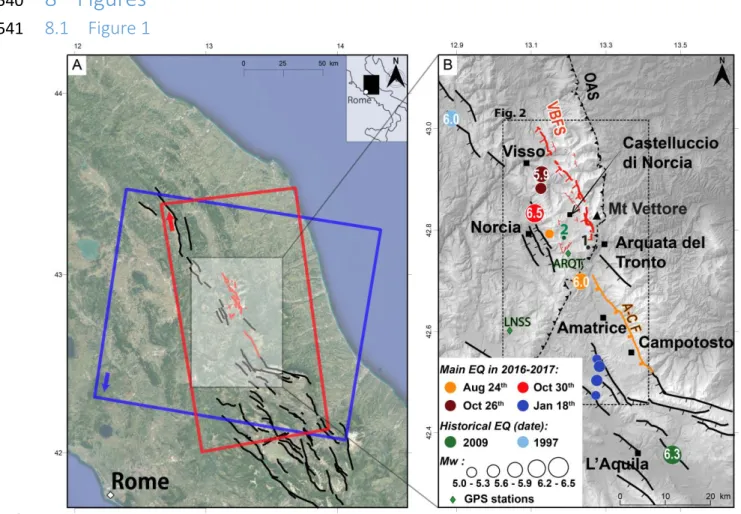
Campotosto event (Figure 1 and Table S1). This seismic sequence ruptured the complex Mt 78

Vettore fault system (in red in Figure 1) (Pizzi et al., 2017; Porreca et al., 2018; Villani, Pucci, et 79

al., 2018), and the adjacent Amatrice-Campotosto fault (in orange in Figure 1). During the 80

Norcia earthquake, the rupturing of an antithetic fault on the opposite side of the Castelluccio 81

basin seems necessary to fit geodetic data and is supported by alignments of relocated 82

aftershocks (Chiaraluce et al., 2017; Walters et al., 2018; Cheloni et al., 2019). In addition, the 83

role of an inherited west-dipping thrust called OAS (Olevano-Antrodoco-Sibillini thrust) in the 84

Norcia earthquake coseismic rupture geometry has been widely discussed. While some studies 85

suggested that only the Mt Vettore fault system was activated (Chiaraluce et al., 2017; Liu et 86

al., 2017; Papadopoulos et al., 2017; Pavlides et al., 2017; Pizzi et al., 2017; Wang et al., 2018; 87

Xu et al., 2017), others suggested that also the OAS thrust ruptured as a reactivated high-angle 88

normal fault during the event, as suggested by geodetic and seismological observations 89

(Cheloni et al., 2017; Scognamiglio et al., 2018; Walters et al., 2018). Although the reactivation 90

of the thrust is not clearly demonstrated (Cheloni et al., 2019), the OAS appears to have played 91

a role in the aftershock distribution (Chiarabba et al., 2018; Chiaraluce et al., 2017; Pizzi et al., 92

2017). The earthquakes of the 2016 sequence appear to have nucleated near crosscutting 93

structures that seem to have been loaded by previous ruptures in the sequence (Chiaraluce et 94

al., 2017; Pino et al., 2019). This seismic sequence is thus an excellent case study to better 95

understand the link between structural segmentation, aseismic slip and frictional properties 96

that might control this rupture propagation. 97

Post–seismic processes during this sequence have been observed in the seismicity (e.g., 98

Albano et al., 2018; Tung & Masterlark, 2018), but no aseismic slip has been detected with 99

geodetic data so far. Using Interferometric Synthetic Aperture Radar (InSAR) time-series from 100

Sentinel-1 data, we document a small but significant post-seismic deformation transient that 101

we find is best explained by aseismic slip on faults associated with this sequence. Surface 102

displacements are presented and analysed. We also explore simple modelling schemes that 103

provide a framework for our interpretation and discussion. 104

2 Geological setting

105

The Central Apennines were affected by an extensional phase during the Jurassic, 106

followed by a compressive phase during the Neogene (e.g., Calamita et al., 2011). The OAS 107

(Olevano-Antrodoco-Sibillini thrust) is one the main thrusts resulting from the Neogene 108

compressive phase (Calamita et al., 1994) and has been interpreted as a transpressive ramp 109

(Di Domenica et al., 2012). In the area affected by the 2016-2017 seismic sequence, the OAS 110

thrust is expressed by parallel splays associated with fault-bend folds characteristic of 111

structural ramps (Calamita et al., 2012) (Figure 1). The ongoing ENE oriented extension of 2 112

to 4 mm/yr (D’Agostino, 2014; Carafa & Bird, 2016; Devoti et al., 2017), which probably began 113

in the Early Pleistocene (e.g., Galadini & Galli, 2000), is currently accommodated through 114

normal fault systems such as the Monte Vettore fault system that hosted the 2016-2017 115

seismic sequence. 116

117

3

Surface displacements during the seismic sequence

118

3.1 InSAR processing

119

Synthetic radar interferometry (InSAR) is now systematically used to constrain 120

deformation fields (Elliott, Walters, et al., 2016) and can document centimetre to millimetre 121

scale slow aseismic ground deformation using an adapted processing chain (Hussain et al., 122

2018; Aslan et al., 2019). We used C band (5.5 cm wavelength) images from Sentinel-1A/B 123

images (Figure 1-A) spanning almost two years (July 28, 2015, to June 11, 2017) for the 124

ascending track (A117, subswath IW3). To confirm the main observations made on the 125

ascending track, we processed descending track (D22, subswaths IW2 and IW3) images from 126

October 26, 2016 to February 11, 2017. SAR images were processed in VV polarization. We 127

used the NSBAS processing chain (Doin et al., 2011, 2015) modified for Sentinel data by 128

Grandin (2015) to generate differential interferograms. The interferogram network, and 129

examples of unfiltered and uncorrected interferograms, are provided in Figures S1 and S2. The 130

Shuttle Radar Topography Mission digital elevation model (DEM) at 3 arc sec resolution (Rabus 131

et al., 2003), resampled at 45m resolution, has been used to accurately coregister the focused 132

SAR images and to correct interferograms from the topographic contribution to the 133

interferometric phase. We removed a ramp in range and in azimuth for each interferogram 134

using the methodology of Cavalié et al., (2007) included in NSBAS. We de-noised the 135

interferograms before unwrapping using collinearity, a criterion to characterize at each pixel 136

the local spatial variability of the phase (Pinel-Puysségur et al., 2012). The collinearity was used 137

to adapt the strength of the filter. We filtered for a window of 12 pixels (400m in range and 138

700m in azimuth); the filter is described in Doin et al. (2011) and is based on the collinearity 139

value which weights the complex phase in a sliding window. For the filter we had the option 140

of adapting the weighting of the phase within windows of different sizes. This size adaptation 141

depends on the collinearity within the windows. Unwrapping was performed in 2D with the 142

NSBAS chain (Grandin et al., 2012; Doin et al., 2015). After unwrapping, to account for errors 143

associated with stratified troposphere, we removed a quadratic cross-function of elevation (z) 144

and azimuth to ramps in azimuth (y) and in range (x) estimation following the function 145

ax+by+c+ez+fz × az+g × (z × az)2 _{using a least-square approach (Daout et al., 2019). Time-series} 146

were then calculated following the NSBAS method (Doin et al., 2011; Daout et al., 2016) using 147

an approach based on the Small Baseline Subset time-series Analysis (SBAS) of López-Quiroz 148

et al., (2009)’s algorithm. The smoothing of the pixel time-series is performed by minimizing 149

the Laplacian of the temporal evolution of the deformation (Cavalié et al., 2007). The final pixel 150

size is 62 m in azimuth and 37 m in range. We removed pixels with an RMS value greater than 151

0.7. For the ascending track, we build a time series spanning the 2 years (from 28/07/2015 to 152

11/06/2017 ) (Figure S1 and see missing links in the time series in Figure S3). For this complete 153

2-year time-series, we encounter problems in unwrapping the co-seismic interferograms due 154

to the large deformation with respect to the Sentinel wavelength in near field (aliasing). 155

Fringes are too close in space and cannot be unwrapped. At pixels that are incoherent in the 156

co-seismic interferogram (i.e. in near field), this causes gaps in the complete (2 yrs) time-series 157

spanning the main earthquakes (Norcia, Amatrice and Campotosto earthquakes) (Figure S3), 158

or lead to an underestimation of the coseismic displacement (brown circles in Figure 2-D). In 159

addition, we also build three time-series in between earthquakes in order to avoid possible 160

bias: before the 24th _{August (Amatrice earthquake), between 27}th _{August and 26}th _October 161

(between the Amatrice and Visso earthquake), and after the 30th _{October (Norcia earthquake).} 162

We excluded the SAR data from January 18, 2017, which produced noised interferograms. For 163

the descending track, we build two time-series: between 27th _{August and 26}th _{October (Visso} 164

earthquake), and after the 30th _{October (Norcia earthquake).} 165

3.2 Time-series results and description of the main features

166

3.2.1 Ascending Track

167

The ascending time-series built before the seismic sequence (from July 28th _{2015 to} 168

August 21th _{2016) does not show significant nor localized surface displacements along the} 169

main faults (Figure S4-A,B). After October 30th_{, the (post-Norcia) time-series shows} 170

centimetre-scale displacements going away from the satellite in the LOS direction in three 171

areas (Figure 2-B): 172

 South of Amatrice: In the area affected by the Campotosto earthquake (January 173

18th_{, 2017 Mw 5.0 -5.5 EQ) the ground surface moved away from the satellite by} 174

more than 60 mm in LOS (Figure 2-B). This coseismic displacement results in a step 175

function in the time series, and can therefore be easily separated from any gradual 176

post-seismic deformation. 177

 Near Arquata del Tronto: At the southern extremity of surface rupture of the Mw 178

6.5 October 30th _{Norcia earthquake (red faults in Figure 2), surface displacements} 179

are detected over an area of ~12 km2_{, and follow logarithmic evolution (in Figure} 180

2-D and Figure 3-A see time-series at point 1 where the cumulative post-Norcia 181

displacements in LOS on January 06, 2017 is in average ~35.5 ± 1.7 mm and reach 182

50.5 ± 2.1 mm on 30 April 2017) 183

 Castelluccio Basin: On the hanging wall of the Mt Vettore fault, slow deformation 184

affects an area of ~50 km2 _{(Figure 2), and is associated with displacements in the} 185

LOS direction that are 13.2 ± 1.4 mm in average at Point 2 on 6 January and reach 186

37.9 ± 1.3 mm on 30 April 2017 (Figure 2-D and Figure 3-A). 187

To rule out possible bias due to the Campotosto earthquakes affecting the area near 188

Castelluccio and near Arquata del Tronto, we confirmed these previous observations with a 189

shorter time-series calculated between the Norcia and Campotosto earthquakes (November 190

1st _{– January 12}th_{) (Figure 4). We prefer to use, for the rest of the manuscript, the longer} post-191

Norcia time-series (November 1st _{– June 11}th_{) that shows a better signal-noise ratio.} 192

In the post Amatrice earthquake time series (August 27 to October 26) we did not observe 193

any localized surface displacements similar to the pattern observed after October 30 (Norcia 194

earthquake) (Figure S4-B). Yet near the town of Amatrice, we observe diffuse surface 195

displacements (< ~2.5 cm) moving away from the satellite. However, this time-series is 196

constrained by only 9 scenes and 20 interferograms, which prevents from properly (i) 197

constraining a low amplitude signal and (ii) correcting for atmosphere and topography. The 198

surface displacements here have a low signal to noise ratio. The variance of the uncorrelated 199

noise is ~ 40 mm2 _{(see Supplementary Text S1 and Figure S5-A), and the standard deviation} 200

sigma of the noise is thus 6.3 mm. We take 3*sigma = 20 mm to set our limit of detection. The 201

characteristic length scale of correlated noise is 5.0 km and there is autocovariance for 202

distances smaller than ~15 km (see Figure S5-A). Observed patterns cannot be differentiated 203

from noise, analyses on SAR images from other satellites should be carried out to confirm or 204

not the post-Amatrice (August 24 earthquake) surface displacements. 205

3.2.2 Descending Track

206

To confirm the post-October 30 (Norcia earthquake) observations we processed 207

descending interferograms (Figure 2-C). We used a 3-month dataset for the descending track 208

(November 1st, 2016 to February 11, 2017). Time-series calculated for the descending track 209

also indicate slow deformation after Norcia earthquake (October, 30), that reaches on average 210

20.5 ± 2.7 mm on January 24 in the LOS direction near Arquata del Tronto (point 1). The 211

deformation reached on average 10.8 ± 1.5 mm in the Castelluccio basin (in point 2). Assuming 212

negligible north-south displacements, by combining the results from ascending and 213

descending tracks, the displacement is dominated by subsidence in this area (Figure S6). 214

In the first order, deformation observed in the descending track is compatible with 215

results inferred from the ascending track. Noise and unwrapping issues led us to mask noisy 216

areas and resulted in more blank pixels in the descending track picture which should be used 217

with caution. The relief projected in the descending LOS geometry masked a ridge (Mt Bove - 218

Mt Vettore – Mt Gorzano high massifs) (Figure S7). In addition to noise, this resulted in an 219

incoherent area and made unwrapping difficult in that area. The temporal evolution of the 220

features slightly differs from the one in the ascending track. The removal of the 7th _November 221

SAR images (affected by strong atmosphere conditions) and the poor constraint on the 19th 222

November SAR images (see the network in Figure S1) could affect the time-series in November. 223

Falcucci et al. (2018) had similar difficulties in using descending SAR images to survey the 224

January 2017 Campotosto seismic event. This might be due to the early morning acquisition 225

time, which amplifies decorrelation due to change of moisture level or thawing. 226

In addition, we produced time-series calculated between the Amatrice and Norcia 227

earthquakes. This time-series is also affected by a short-wavelength atmospheric turbulence 228

that makes it difficult to interpret (Figure S5-B-C). The variance of noise is ~21 mm2_{. The} 229

characteristic length scale of correlated noise is 5.0 km and there is autocovariance for 230

distances smaller than ~15 km (see Figure S5). Again, displacement less than 19 mm for the 231

ascending track and under 14 mm for the descending track, cannot be considered as 232

detectable signal, therefore constraining smaller surface displacements between the Amatrice 233

and Norcia events demands complementary time-series with SAR images from other satellite. 234

3.2.3 Comparison with GNSS

235

Few GNSS stations exist near the studied area (ARQT, LNSS see station locations in Figure 236

2-A). Those GNSS time-series agree with InSAR time-series sampled at the same locations 237

(Figure S8). 238

3.3 Pattern temporal evolution

239

By sampling the time-series, the temporal evolution is shown by averaging pixel 240

displacement in area. To enhance the precision of the displacement temporal evolution 241

without using time-series inversion, we temporally track a stable pattern in our unwrapped 242

interferograms (Grandin, 2009). The method is detailed in Supplementary Text S2 and is 243

illustrated by Figures S9-S10. 244

This method can only be used on areas where the displacement pattern is well defined, 245

and works well in our case to track the evolution of the area near Arquata del Tronto (pattern 246

in Figure 4 which encompasses the point 1). After the Norcia earthquake, the amplitude ratio 247

is higher, and a logarithmic decay is clearly identified there (Figure 3-B). The pattern tracking 248

shows a temporal evolution similar to the averaging surface displacement method. We are 249

therefore confident that pixel averaging adequately captures the evolution of displacement 250

that we want to describe. For the descending interferograms, the pattern is not precisely 251

trackable and its time evolution is noisy (grey curve in Figure S10-C). This could be due to a 252

poor correlation for the pattern in some interferograms. The evolution of the pattern around 253

Castelluccio Basin (pattern in Figure 4) is poorly resolved too. 254

4 Modelling 3D deformation field

255

4.1 Comparison with topography and geology

256

To interpret the displacement pattern near Arquata del Tronto we compared it with the 257

topography and the geology. There is no correlation with either the slope or the relief (Figure 258

S11), thus we can exclude a gravitational process (i.e. landslide) as an explanation for the 259

observed displacements. Concerning geology, the OAS thrusts fractured Meso-Cenozoic 260

carbonate rocks over Neogene pelagic sediments; the carbonates host some of the largest 261

aquifers in the Apennines while the Neogene sediments are thought to be an aquiclude (Figure 262

S12) (Boni et al., 2010). The OAS delimiting these two units therefore acts as an impermeable 263

boundary (Boni et al., 2010). Petitta et al., (2018) and Valigi et al., (2019) show that the 2016-264

2017 Italian seismic sequence had effects on spring discharge, water-table levels, and 265

streamflow of those aquifers. In our results, the extent of the Maiolica unit, which hosts a 266

shallow aquifer (Boni et al., 2010), corresponds well with the deformation area near Arquata 267

del Tronto (Figure S11-A-B). The long pre-seismic InSAR time-series did not show any seasonal 268

deformation in this aquifer, which means that groundwater seasonal processes can be 269

excluded (point 1 in Figure 2-D). In addition, it seems difficult to get more than 1 cm of 270

subsidence from winter rain in this area (i.e., Silverii et al., 2016). 271

4.2 Poro-elastic modelling

272

Poro-elastic effects have been studied during the 2016-2017 seismic sequence to explore 273

the aftershocks and earthquakes triggering. Tung & Masterlark (2018) suggest that fluid 274

migration caused by the Amatrice earthquake (August 24, 2016) could have triggered the Visso 275

earthquake (October 26, 2016), as well as some associated aftershocks. They inferred that this 276

poro-elastic triggering should have occurred in an intermediately fractured crust. They also 277

estimated that afterslip and viscoelastic-relaxation were quite negligible with respect to 278

poroelastic effects. Albano et al. (2018) also suggest that post-seismic fluid diffusion after the 279

Amatrice earthquake is related to aftershocks. According to their pore fluid diffusion model, 280

there could be some associated afterslip (~ 10 cm) after the Amatrice earthquake. 281

The Maiolica karst aquifer is shallow and unconfined but Roeloffs (1996) postulates that 282

every aquifer reacts as a confined aquifer to a disturbance at short timescale. Here, to compare 283

with the displacement pattern near Arquata del Tronto, we thus test a forward model of poro-284

elastic rebound using Relax software (Barbot & Fialko, 2010). We perform a simple poro-elastic 285

model with no lateral variation of diffusivity, that does not account for the spatially 286

heterogeneous distribution of local aquifers. We use the slip distribution models of the Norcia 287

and Visso mainshocks (Maubant et al., 2017), (Figure S13 and Figure 5–A). We do not take into 288

account the Amatrice earthquake since poroelastic rebound from the Amatrice earthquake 289

would likely have stabilized by the time of the Visso and Norcia earthquakes (Figure 4-f in 290

Albano et al., (2018)). We tested several diffusivities for a shallow layer (0-5 km depth), from 291

1.5 m².s proposed by the Tung and Masterlark (2018)’s aftershocks analysis to 104 _m²/s 292

(maximum diffusivity value for karst) (Roeloffs, 1996). Other parameters are described in detail 293

in Figure 5. This model predicts uplift in the Castelluccio Basin and near Arquata del Tronto 294

(Figure 5-D) where we observe subsidence (Figure 5-C). This discrepancy allows us to rule out 295

poro-elastic rebound as the main driver of observed deformation. These poroelastic models 296

are not exhaustive, we only explore simple geometrical configurations using parameter values 297

informed by the local geology, however, other karstic configurations would likely predict uplift 298

as well. 299

4.3 Viscoelastic modelling

300

Viscoelastic relaxation in the crust and in the mantle is also an important aseismic 301

process, and has been inferred to be the driver of post-seismic deformation following many 302

earthquakes (e.g., Pollitz et al., 2001; Zhao et al., 2017). To test whether viscoelastic relaxation 303

is a plausible driving mechanism for post-Norcia deformation, we used Relax to perform 304

forward modelling in a simple layered framework. Our model uses the stress perturbation 305

from the three mainshocks: the Amatrice earthquake using the slip distribution of Ragon et 306

al., (2019) added to the Visso and Norcia earthquakes using the slip distribution model of 307

Maubant et al., (2017). We set the upper, middle and lower crust thickness to the values 308

proposed in Laske et al., (2013) and Verdecchia et., al. (2018) (see Table 1). We tested a 309

viscoelastic relaxation governed by a Newtonian rheology with 𝛾̇ =𝜏

𝜂 where 𝛾̇ is the viscous

310

strain rate, τ is the deviatoric stress and η is the Newtonian viscosity. We used viscosity values 311

η inferred in studies of viscoelastic relaxation modelling using GPS measurements following 312

1997 Umbria-Marche earthquakes, or using levelling line measurements following the 1915 313

Fucino earthquake (Amoruso et al., 2005; Aoudia et al., 2003; Riva et al., 2007). These studies 314

inferred that the ductile structure of the Central Apennines consists of an elastic upper crust 315

overlaying a middle crust (1018_-1019 _{Pa s), a viscous lower crust (10}17_-1018 _{Pa s) and the upper} 316

mantle (1021 _{Pa s) (Table 1).} 317

Although those models are geometrically simple and do not take into account 318

earthquakes prior 2016, they predict at a long-wavelength uplift (>50 km) in the area where 319

we observe subsidence (Figure 6). This discrepancy in both sign and wavelength allows us to 320

rule out a simple visco-elastic relaxation as the main driver of observed deformation. Visco-321

elastic models are not exhaustive here: nonlinear viscoelastic rheologies (e.g., power law 322

creep) in lower crust (Freed & Bürgmann, 2004) could also be investigated; however finite 323

element models with creeping lower crust seem also to predict uplift in similar settings of 324

normal fault systems (e.g., Thompson & Parsons, 2016). It is worth also mentioning that the 325

observed logarithmic decay could also potentially be associated with Burgers rheology or shear 326

zone (e.g., Hetland & Zhang, 2014) and could also be investigated in future work. Although, as 327

with the poroelastic modeling, it seems unlikely that a different geometry or rheology could 328

completely reverse the sign of uplift and subsidence (for example, a different rheology would 329

only affect the temporal evolution/spatial distribution). 330

4.4 Modelling the temporal evolution of afterslip

331

The logarithmic-like temporal evolution of displacement (Figure 3-A), and the 332

disagreement between the observations and the predictions of poroelastic and viscoelastic 333

models, suggest that afterslip may have been the main driver of postseismic deformation 334

(Marone et al., 1991). Thus to characterize the temporal evolution of the deformation, we 335

fitted the deformation decay (of the raw time-series and of the pattern tracking evolution) 336

with the logarithmic function (Figure 3-A-B respectively) from the Marone et al. (1991) model 337

and Zhou et al. (2018) reformulation for rate-strengthening afterslip: 338 𝑈(𝑡) ≈ 𝛼 × ln(1 + 𝑐 × 𝑡) 339 𝑐 =𝛽 × 𝑉𝑖 𝛼 340

In which U: afterslip in time t, α: characteristic length scale, β× 𝑉_𝑖 : initial rate at the 341

beginning of the post-seismic period, with 𝛽 a scaling vector by which the sliding rate evolves 342

in response to the stress and 𝑉_𝑖 the pre-seismic slip rate. 343

At point 1 (near Arquata del Tronto), the good fit of the afterslip model suggests that the 344

main post-seismic process is likely an afterslip phenomenon. Since we found similar results for 345

c value (describing the temporal decay) using the raw pixel time series and using the pattern 346

tracking (independent for the time-series inversion), we are confident in our fitting (Table 2). 347

The first post-Norcia Sentinel image has been acquired 2.6 days after the Norcia earthquake; 348

therefore those 2.6 days of early afterslip are missing in our data. We compare the temporal 349

decay of the deformation with the cumulative moment and number of aftershocks (blue and 350

green curves in Figure S14). Although the completeness magnitude is high (ML 3 in Figure S5 351

in Chiaraluce et al., (2017)), those two curves obtained with less than 50 events are not 352

following the same trends, aftershocks do not seem to be induced by afterslip. At point 2 (near 353

Castelluccio di Norcia), the temporal decay does not fit with the afterslip law as the rate at the 354

beginning of the post-seismic period is close to zero (c value for the purple curve fit in Figure 355

3-A). Other post-seismic processes could be a complementary driver of the deformation here 356

and should be taken into account in further modelling (i.e. finite element forward model 357

accounting for afterslip superimposed with poro-elastic rebound and viscoelastic relaxation). 358

4.5 Afterslip modelling on faults

359

4.5.1 Inversion strategy and fit to the data

360

To obtain the afterslip distribution we use the Classic Slip Inversion (CSI) Python tools 361

(Elliott, Jolivet, et al., 2016; Jolivet et al., 2015) to invert for the slip. We use the constrained 362

least-squares formula of Tarantola (2005) to solve the inverse problem (see details in 363

Supplementary Text S3 and Figures S15 to S18). We chose a dip of 40° for the Mt Vettore fault 364

(as Cheloni et al., (2017) see Figure S15) and project the fault down dip from the mapped fault 365

at the surface (modeled fault geometry in yellow Figure 2-A). We discretize the fault into 88 366

rectangular patches. The smoothed cumulative surface displacement on February 11, 2017, 367

measured in both ascending and descending tracks are inverted to obtain the afterslip 368

distribution. The resolution is good for short-wavelength features at shallow depths (<5 km 369

depth) (Figure S16). As several geometries have been used to model the mainshock rupture 370

(OAS reactivation, antithetic fault), we explored three cases: (1) slip only on the Mt Vettore 371

Fault, (2) slip on the Mt Vettore Fault and on the OAS and (3) slip on the Mt Vettore Fault and 372

an antithetic fault with a geometry similar to the one proposed by Cheloni et al., (2019) and 373

Maubant et al., (2017) (dip 65°) (Figures S17 to S20). We also explored the rake: (1) dip-slip 374

only and (2) variable rake. A rigorous statistical comparison between the cases is difficult due 375

to variation in model parameters and number of degrees of freedom, as explained by Cheloni 376

et al., (2019). We thus used the RMS values to compare the different cases. Here the case that 377

reduces the residuals the most is the inversion with an antithetic fault. This case is in addition 378

consistent with geological and seismological observations (i.e. Cheloni et al., 2019). The 379

different cases were compared using the RMS (root mean square), and allows us to choose the 380

inversion with an antithetic fault (Table S2). 381

Both ascending and descending tracks are well modelled (Figure 7). It is worth noting 382

that the resolution is low at depth (Figure S16). The total geodetic moment released by the 383

afterslip model is equivalent to Mw ~5.78 (without taking into account the Campotosto 384

earthquake) which corresponds to ~8.7% of the geodetic moment released during the Norcia 385 earthquake (Mw 6.5). 386 387 4.5.2 Afterslip distribution 388

4.5.2.1 Near Arquata del Tronto

389

We obtain a maximum afterslip of ~100 mm below Arquata del Tronto at shallow depth 390

(0- 2 km depth) (Figure 7 Figure 8). The shallow part depth < 3-4 km toward the south is 391

associated with very low coseismic slip for both the Norcia and Amatrice earthquakes and is 392

located at the edge of the coseismic asperities. This is also consistent with an afterslip process: 393

the afterslip is located where the slip gradient increased the shear stress on the unruptured 394

portions. This feature has also been observed after the L’Aquila earthquake (D’Agostino et al., 395

2012). We calculate a geodetic moment released equivalent to Mw ~5.1 in this area (patches 396

above 2km depth and south of Arquata del Tronto). The cumulative moment released by the 397

seismicity (Figure S14-D) at this date corresponds to ~2.0% of the moment released by the 398

afterslip model. The deformation is thus mainly aseismic. 399

Brozzetti et al., (2019) found some surface ruptures south of the 30th _{October Norcia} 400

rupture (42°47’N in their Fig. 1-C) mapped by Villani et al., (2018). The ruptures mapped by 401

Brozzetti et al., (2019) are subtle and according to us may correspond to post-seismic 402

deformation, as was observed after the L’Aquila earthquake (D’Agostino et al., 2012). 403

4.5.2.2 Castelluccio Basin

404

We observe a maximum slip of ~ 170 mm below Castelluccio at ~5 km depth. Some 405

afterslip overlaps with the coseismic rupture area, but not in the area of maximum coseismic 406

slip (Figure 7). As also the shape of the measured time-series did not fit with the afterslip’s law 407

(Figure 3-A), a sole afterslip process is unlikely. It is possible that poroelastic and fluid flow 408

processes could be at work here since there is a large basal aquifer (Boni et al., 2010). 409

Modelling accounting for both processes could be performed, for example fully coupled 410

poroelastic finite element numerical modelling with spatially variable material properties (e.g., 411

Albano et al., 2017). 412

5 Discussion

413

5.1 Afterslip mechanism near Arquata del Tronto

414

Based on Dietrich (1979), Ruina (1983) and Marone et al., (1991) equations, we 415

estimated 𝛼 (the characteristic length scale over which the elastic stress changes by order of 416

the frictional stress) in Figure 3 and Table 2. We can now estimate the friction 417

parameter (𝑎 − 𝑏) since according to Perfettini and Avouac (2004) and Zhou et al., (2018): 418

𝛼 =(𝑎 − 𝑏) × 𝜎 𝑘 419

420

with k: the effective stiffness, and 𝜎 the effective normal stress. This relation can be applied 421

to our case since the duration of our analysis (~200 days) is much shorter than the 422

characteristic time td (Gualandi et al., 2014). Where td= 𝛼

𝑉𝑝𝑙 (>12 years) where Vpl is the local

423

plate loading rate (<2.1 mm/yr (Puliti et al., 2020)). The fit to the displacement of the time-424

series sampled in point 1 by an afterslip law (Figure 3) leads to α= 30.9±4.0 mm. To estimate 425

σ, we assume that the mean normal stress may vary from the hydrostatic to lithostatic 426

pressure, with a rock density of 2.5 kg.m-3 _{(Albano et al., 2018) and a depth of the slipping area} 427

of 3-5 km. This leads to σ = 44-124 MPa. For k =G/h with G=30 GPa (the shear modulus near 428

the surface) and h=8 km (rate-strengthening depth based on the coseismic slip models), we 429

obtain (a-b)=3 x 10-3 _{- 7.8 x 10}-4_{. More complex models (e.g. finite element model,} 430

heterogeneous (a-b) values) could be performed by future studies in order to reproduce the 431

surface displacements and to propose a more precise value of (a-b). However, our estimation 432

is in agreement with experiments on carbonates. Scuderi and Collettini (2016) found values of 433

(a − b) evolve from velocity strengthening behaviour (a − b ≈ 0.005) at fluid pressure condition 434

of sub-hydrostatic to a velocity neutral behaviour (a − b approaching 0), when the fault is at 435

near lithostatic fluid pressure. Pluymakers et al., (2016) found that wet anhydrite and dolomite 436

gouges at depths <6 km, exhibit (a-b) values ranging from 10-2 _{to 10}-4_. 437

In Arquata del Tronto, the obtained (a-b) positive value (0.0026) is in agreement with 438

a velocity-strengthening area. The obtained (a-b) value is also very low and corresponds to a 439

quasi-neutral rate-dependency of friction implying a high sensitivity to stress perturbations. 440

Potential stress perturbations needed to reach strengthening may involve either a decrease in 441

effective normal stress and / or an increase in shear stress (Scholz, 1998). Walters et al., (2018) 442

calculated the Coulomb stress change (CFF) after the Norcia earthquake. At shallow depths, 443

they found a positive CFF change below Arquata del Tronto, which might have triggered the 444

observed afterslip in this area. An increase in pore fluid pressure would have a similar effect. 445

The afterslip is located near to the Olevano-Antrodoco-Sibillini (OAS) thrust. Chiarabba et al., 446

(2018) detected a high Vp/Vs near the OAS thrust (around 3 km depth), indicating high pore 447

pressure that could have been further increased by nearby major shocks (Amatrice and Norcia 448

earthquake). This high pore pressure could have induced the observed afterslip allowing for 449

the release of the residual accumulated stress. This scenario is also supported by the fact that 450

pore fluid pressure variation is common in this area, where the inherited structures seem to 451

control the rupture pattern and could also concentrate high shear stress. Future work could 452

examine detailed Coulomb Stress modelling with high spatial resolution taking all fault 453

complexity and pore fluid effects into account. These works could be useful, despite some 454

limitations related to the resolution of the coseismic slip and by the ambiguity about which 455

faults were involved. 456

If this overlapping of coseismic slip and afterslip is real below 4-5 km depth (below 457

Arquata del Tronto) could be an artefact caused by the smoothing used to regularize the 458

inversion of the slip distribution, combined with the fact that the resolution at depth is limited. 459

If this overlapping of co-seismic and slow slip was confirmed, a simple interpretation of rate 460

and state friction cannot be proposed here. Overlaps between coseismic slip and afterslip have 461

been observed after several earthquakes. For example after 2004 MW 6 Parkfield earthquake, 462

afterslip was inferred to overlap the coseismic slip (Freed, 2007). Johnson et al., (2006) 463

proposed frictional spatial heterogeneity to explain the afterslip distribution, and proposed (a-464

b) values on the order of 10-4 _{– 10}-3_{. After the 2015 Ilapel MW 8 megathrust earthquake,} 465

Barnhart et al. (2016) also observed afterslip and coseismic slip overlapping, and advocated 466

that stress heterogeneities likely provide the primary control on the afterslip distribution. After 467

the 1978 MW 7.3 Tabas-e-Golshan earthquake, Zhou et al., (2018) also observe such 468

overlapping and found (a-b)~3.10-3_{. They proposed that the fault is creeping during the whole} 469

interseismic period and that the earthquake propagates through the rate-strengthening region 470

although they also stated that a change in frictional properties is also possible due to shear 471

heating. Thomas et al., (2017), after the 2003 MW 6.8 Chengkung earthquake estimated that 472

(a-b) varies with depth from 0.018 near the surface to less than 0.001 at depth larger than 19 473

km, to explain areas showing both seismic and aseismic behavior they advocated shear heating 474

processes. Using numerical modelling, Noda and Lapusta (2013) argued that coseismic slip 475

could propagate into velocity-strengthening regions of a fault, and that these regions can 476

appear locked or creeping during the interseismic period. They observed this behavior due to 477

rapid shear heating. For our case it is difficult to pinpoint the particular fault zone mechanism 478

here, but we can proposea switch to (a-b) positive value below 4-5 km depth, due to coseismic 479

shear heating processes (Thomas et al., 2017) requiring temperature changes of several 480

hundred degrees (e.g., Rice, 2006). This could be a potential explanation since Smeraglia et al., 481

(2017) suggested that nanostructures from the Mt Vettoreto Fault rocks were generated by 482

coseismic shear heating and grain comminution (reduction of particle sizes). 483

484

5.2 Barrier of rupture propagation

485

Near Arquata del Tronto, at shallow depth (< 3-4 km) we observe that the aseismic slip is 486

localized on an area associated with limited coseismic slip, for both the Amatrice and Norcia 487

earthquakes. The observed aseismic slip seems located in an area where coseismic ruptures 488

have not propagated during the Norcia or Amatrice earthquakes. This slowly slipping zone is 489

located near a structural complexity (inherited thrust OAS), that Chiaraluce et al., (2017), Pizzi 490

et al., (2017) and Puliti et al. (2020) interpreted as a barrier that concentrated stress after the 491

Amatrice earthquake. We propose that maybe as a result of this geometric complexity (that 492

may concentrate high stress and high porosity resulting from fracturation), this zone might be 493

also characterized by frictional properties at shallow depth that could have favoured the arrest 494

of the ruptures (e.g., Kaneko et al., 2010). Scholz (1998) shows that when an earthquake 495

propagates into a velocity strengthening field it will produce a negative stress drop, that rapidly 496

terminates propagation. Our simple calculations yield here a slightly positive (a-b) value, 497

consistent with this model. 498

6 Conclusion

499

The Sentinel-1 InSAR time-series show cm-scale post-seismic displacements after the 500

Norcia earthquake (October 30). The displacements are more obvious in the ascending track 501

than in the descending track, and correspond to ~1 to 5 cm of subsidence in the Castelluccio 502

basin and at the southern tip of the Norcia surface rupture. In the area of the Castelluccio 503

basin, whether the deformation can be explained by afterslip only is less clear and would 504

require additional modelling to include the effects of poro-elastic release or shear zone 505

deformation. At the southern edge of the Norcia coseismic rupture, deformation evolves with 506

time following a logarithmic decay consistent with afterslip triggered by the Norcia 507

earthquake. Although good observations of the 2.6 first days of afterslip are not available, after 508

3 months the slow deformation evidenced in this study released a geodetic moment of Mw 509

~5.78, which corresponds to ~8.7 % of the geodetic moment released during the Norcia 510

earthquake. Cumulated moment released by aftershocks in the southern tip of the Norcia 511

rupture accounts for ~2.0 % of the moment released by the modelled deformation, the 512

deformation is thus here mainly aseismic. This afterslip takes place at the southern tip of the 513

Norcia rupturing patch, and seems to have acted as a barrier to the propagation of Norcia and 514

Amatrice ruptures at shallow depth (<3-4 km). Our results suggest that the observed post-515

Norcia earthquake afterslip might have been triggered in response to heterogeneities of pore 516

fluid pressure, potentially facilitated by structural complexity and intense faulting in the area. 517

Such small and localized slow deformation due to afterslip may be best detected with InSAR 518

time-series in regions of sparse GNSS coverage. It might actually be quite common and could 519

be an underestimated phenomenon. This likely points toward a bias in the literature in favour 520

of high and wider afterslip, that is easier to detect. However detection of small afterslip 521

transient is crucial to further understand the physics of earthquakes, and the link between 522

slow slip and seismic rupture (e.g., Kaneko et al., 2010; Rousset et al., 2017). 523

7 Tables

Depths (km) Model 1 η Model 2 η Model 3 η Model 4 η Upper crust 0-10.7 Elastic Elastic Elastic Elastic

Middle crust 10.7-21.7 Elastic 1019 _{Pa s 10}18 _{Pa s 10}18 _{Pa s}

Lower crust 21.7-33.1 1018 _{Pa s 10}18 _{Pa s 10}18 _{Pa s 10}17 _{Pa s}

Upper mantle 33.1-below 1021 _{Pa s 10}21 _{Pa s 10}21 _{Pa s 10}21 _{Pa s} 529

Table 1 : Crust and mantle viscosities (η) tested in Figure 6. 530 531 532 7.2 Table 2 533 534 Fit α C (days-1_{) γ R2}

Point 1 near Arquata del Tronto

30.9 ± 4.0

0.26 ± 0.26 -6.4 ± 6.2 0.87

Point 2 near Castelluccio di Norcia

156.4 ± 230.7

0.003 ± 0.007 2.54 ± 3.5 0.81

Pattern tracking 1.6 ± 0.1 0.24 ± 0.1 -0.37 ± 0.21 0.95 535

Table 2: Parameters obtained from the fit of the afterslip model in Figure 3 using a non-linear 536

least squares method (Moré, 1978). R2 is the coefficient of determination of the regression. 537

The pattern encompasses the point 1 (see Figure 4) 538

8 Figures

540

8.1 Figure 1

541

542

Figure 1: Neotectonic framework of the Central Apennines. Black lines are main normal active 543

faults compiled from Benedetti (1999), Tesson et al., (2016) and references therein (VBFS: Mt 544

Vettore – Mt Bove Fault System, A-C F: Amatrice-Campotosto Fault). In red, coseismic surface 545

ruptures observed in the field after the mainshocks of the Central Italy 2016-2017 seismic 546

sequence (Villani, Civico, et al., 2018). (A) Blue and red rectangles are, respectively, the 547

descending (D22 subswaths IW2 and IW3) and ascending (A117, subswath IW3) Sentinel tracks 548

processed in this study. (B) Black dashed line represents the Neogene OAS thrust (Olevano-549

Antrodoco-Sibillini thrust) (Di Domenica et al., 2012). In orange the Amatrice-Campotosto fault 550

which was activated during the 2016—2017 seismic sequence. ARQT and LNSS (in B) are GNSS 551

stations available in this region from

552

http://geodesy.unr.edu/NGLStationPages/gpsnetmap/GPSNetMap_MAG.html (Blewitt et al., 553

2018). 554

8.2 Figure 2

556

557

Figure 2: (A) Map of the studied area, green squares are the GPS stations, points 1-2 are the 558

points of sampling. The modeled geometries of the Mt Vettore and antithetic faults are plotted 559

(see section 4.5). Circles are the earthquakes (see Figure 1). (B-C): Time-series calculated 560

cumulative post-Norcia (30 oct) displacements for ascending (B) and descending track (C), 561

respectively. In panels A,B,C,E : Red lines are surface ruptures associated with 30th _October 562

2016 Norcia earthquake (Villani, Civico, et al., 2018), and black lines are active faults. Black 563

dashed line is the OAS thrust. (VBFS: Mt Vettore – Mt Bove Fault System, A-C F: Amatrice-564

Campotosto Fault, OAS: Olevano-Antrodoco-Sibillini thrust). (D) Displacement through time 565

averaged over a circle of 20 pixels (dashed circles in panel E) in diameter around points 1-2. (E) 566

Cumulative displacement on June 11, 2017, with respect to the 1st _{November 2016 date.} 567

8.3 Figure 3

569 570

571 572

Figure 3: (A) Temporal variation of displacement averaged over a circle of 20 pixels in diameter 573

through time of point 1 (black curve) and 2 (purple dashed curve) localized in Figure 2-E. We 574

fitted the curve with afterslip model (see results in Table 2). 575

(B) Temporal variation of pattern amplitude. Pattern is indicated in Figure 4. In red, the fit with

576

an afterslip model (see results in Table 2). 577

578 579

580

8.4 Figure 4

581

582

Figure 4: Mean velocity map between Mw 6.5 Norcia and Mw 5.7 Campotosto earthquakes 583

(November 1st _{– January 12}th_{). This map is computed using 35 ascending interferograms. The} 584

swath A-B is used in Figure S11 to compare InSAR displacements and topography. Circles 585

represent the earthquakes (see color code in Figure 1). 586

587 588

8.5 Figure 5

589

590

Figure 5: Poro-elastic rebound modelled with Relax software (Barbot & Fialko, 2010). We used 591

the coseismic slip models of the Norcia and Visso earthquakes from Maubant et al., (2017). 592

(A) Mapview of the coseismic slip distribution. (B) Coseismic –σkk modelled at 500m depth,

593

calculated in an undrained homogenous elastic medium (Poisson ν=0.34; Lamé λ=6.36E+04 594

MPa, shear modulus G=30 GPa, Gravity wavelength γ=5.39E-04 km-1_{). To remind, the pore} 595

pressure change (Δp) is equal to -B*σkk/3, with (B the Skempton’s coefficient). (C) Post-Norcia 596

cumulative displacement map (11th _{February 2017) observed by InSAR (uplift component). (D)} 597

Model-predicted poro-elastic rebound as of 25th _{February 2017, obtained using the difference} 598

between drained and undrained conditions. Poisson drained is 0.26 (cf. layer 1 in Albano et al. 599

2018), and for undrained conditions is 0.34 (from beta=0.4 in the table 1 and equation 15 in 600

Barbot et al., (2010)). The layer between (0 and 5 km) is characterized by a diffusivity equals 601

to 1.5 m²/s (Tung & Masterlark, 2018). (E) Modelled poro-elastic rebound time-series at point 602

A using several diffusivities, from 1.5 m²/s (Tung & Masterlark, 2018) to 104 _{m²/s (Roeloffs,} 603

1996). Because the delay time is inversely proportional to the assumed diffusivity, the 604

response for high diffusivity is shorter. (VBFS: Mt Vettore – Mt Bove Fault System, A-C F: 605

Amatrice-Campotosto Fault, OAS: Olevano-Antrodoco-Sibillini thrust). 606

8.6 Figure 6

608

609

Figure 6: Surface displacements predicted by visco-elastic models, we used the Amatrice, 610

Norcia and Visso earthquakes coseismic slip distribution modelled by Ragon et al., (2019) and 611

Maubant et al., (2017). (A) Coseismic slip distribution of the Amatrice earthquake from Ragon 612

et al., (2019) (B-C-E-F) Surface displacements predicted by four visco-elastic models on 24th 613

February 2017 using Relax software (Barbot & Fialko, 2010). Mantle viscosity is fixed for all 614

models at 1021 _{Pas. (D) Post-Norcia earthquake (30}th _{October) cumulative displacement map} 615

(11th _{February 2017) observed by InSAR (uplift component). (VBFS: Mt Vettore – Mt Bove Fault} 616

System, A-C F: Amatrice-Campotosto Fault, OAS: Olevano-Antrodoco-Sibillini thrust) 617

618 619

8.7 Figure 7

620 621

622

Figure 7: Result of afterslip inversion using the CSI software (see Supplementary text S3 for 623

details). (A) Subsampled displacement maps for the ascending (left column) and descending 624

(right column) tracks. Top row shows the input subsampled data, middle row shows the 625

synthetic displacements predicted by the model, and bottom row shows the residuals (i.e. 626

model - data). The modeled fault geometries used for the inversion are plotted in Figure 2-A. 627

The input maps are the smoothed cumulative displacement maps on February 11th _(calculated 628

in the ascending and descending post-30th _{October time-series). (B) Afterslip distribution} 629

inverted from the data on the main fault and the antithetic fault. Black arrows in patches show 630

the rake. Our model has low resolution at depth (Figure S16). Coseismic slip distributions for 631

the Amatrice and Norcia earthquakes (Scognamiglio et al., (2018) are superimposed in white 632

and red , respectively. Comparison with the Cheloni et al.,(2019) model in Figure S21 shows 633

similar patterns. 634

635 636

8.8 Figure 8

637

638

Figure 8: Afterslip distribution model plotted on mapview. The slip distribution is inverted from 639

the data on the main fault and the antithetic fault (see Figure 7). (VBFS: Mt Vettore – Mt Bove 640

Fault System, A-C F: Amatrice-Campotosto Fault). Circles are the main earthquakes of the 641

seismic sequence. 642

9 Acknowledgments

644

We would like to thank the Editor, Associate Editor, Mong-Han Huang and two anonymous

645

reviewers for their constructive suggestions, which helped to improve the manuscript substantially. We

646

acknowledge the French Spatial Agency CNES (Centre National d'Etudes Spatiales) for funding this

647

study (Program THEIA and CNES post-doctorate fellowship for L.Pousse-Beltran). This work was also

648

funded through the TELLUS-ALEAS program from Institut des Sciences de l'Univers (INSU). CNES is

649

warmly acknowledged from providing us with the Pléaides satellite images through ISIS and

650

CEOS_seismic pilot (ESA) programs. Nicola D’Agostino was under an invited researcher position at Univ.

651

Grenoble Alpes - OSUG - ISTerre when most of the work was performed. Most of the computations

652

presented in this paper were performed using the Luke platform of the CIMENT infrastructure

653

(https://ciment.ujf-grenoble.fr), which is supported by the Rhône-Alpes region (grant CPER07_13

654

CIRA), the OSUG@2020 labex (reference ANR10 LABX56), and the Equip@Meso project (reference

655

ANR-10-EQPX-29-01) of the programme Investissements d’Avenir supervised by the Agence Nationale

656

pour la Recherche. Franck Thollard, Christophe Laurent, Erwan Pathier, Louise Maubant and Simon

657

Daout are warmly acknowledged for help and advice on NSBAS processing chain. We are also grateful

658

to Théa Ragon and Romain Jolivet for support and advice in slip distribution modelling, the CSI software

659

will be soon released online. We thank Louise Maubant and James Hollingsworth for sharing the Norcia

660

slip distribution model. Alberto Pizzi, Bruno Pace, Paolo Boncio and Irene Puliti are also warmly

661

acknowledged for fruitful discussions. The European Space Agency (ESA) Copernicus program has

662

provided free and high-quality SAR data from Sentinel-1A and 1B (ESA, 663

https://scihub.copernicus.eu) through the PEPS platform of CNES (Copernicus 2018 for Sentinel

664

data. We thank Simone Tarquini for the supply of 10 m resolution TINITALY DEM. The afterslip

665

distribution model will be provided in 10.5281/zenodo.3755127 . Seismicity used for this research is

666

included in (Chiaraluce et al., 2017) and in http://cnt.rm.ingv.it/. The GNSS stations are downloaded

667

from http://geodesy.unr.edu/NGLStationPages/stations/

668 669

10 References

670 671

Albano, M., Barba, S., Solaro, G., Pepe, A., Christian, B., Moro, M., et al. (2017). Aftershocks, 672

groundwater changes and postseismic ground displacements related to pore pressure 673

gradients: Insights from the 2012 Emilia-Romagna earthquake. Journal of Geophysical 674

Research: Solid Earth, 122(7), 5622–5638. https://doi.org/10.1002/2017JB014009 675

Albano, M., Barba, S., Saroli, M., Polcari, M., Bignami, C., Moro, M., et al. (2018). Aftershock 676

rate and pore fluid diffusion: Insights from the Amatrice-Visso-Norcia (Italy) 2016 677

seismic sequence. Journal of Geophysical Research: Solid Earth, 0(ja). 678

https://doi.org/10.1029/2018JB015677 679

Amoruso, A., Crescentini, L., D’Anastasio, E., & Martini, P. M. D. (2005). Clues of postseismic 680

relaxation for the 1915 Fucino earthquake (central Italy) from modeling of leveling 681

data. Geophysical Research Letters, 32(22). https://doi.org/10.1029/2005GL024139 682

Aoudia, A., Borghi, A., Riva, R., Barzaghi, R., Ambrosius, B. a. C., Sabadini, R., et al. (2003). 683

Postseismic deformation following the 1997 Umbria-Marche (Italy) moderate normal 684

faulting earthquakes. Geophysical Research Letters, 30(7).

685

https://doi.org/10.1029/2002GL016339 686

Aslan, G., Lasserre, C., Cakir, Z., Ergintav, S., Özarpaci, S., Dogan, U., et al. (2019). Shallow Creep 687

Along the 1999 Izmit Earthquake Rupture (Turkey) From GPS and High Temporal 688

Resolution Interferometric Synthetic Aperture Radar Data (2011–2017). Journal of 689

Geophysical Research: Solid Earth, 124(2), 2218–2236.

690

https://doi.org/10.1029/2018JB017022 691

Avouac, J.-P. (2015). From Geodetic Imaging of Seismic and Aseismic Fault Slip to Dynamic 692

Modeling of the Seismic Cycle. Annual Review of Earth and Planetary Sciences, 43(1), 693

233–271. https://doi.org/10.1146/annurev-earth-060614-105302 694

Barbot, S., & Fialko, Y. (2010). A unified continuum representation of post-seismic relaxation 695

mechanisms: semi-analytic models of afterslip, poroelastic rebound and viscoelastic 696

flow: Semi-analytic models of postseismic transient. Geophysical Journal International, 697

182(3), 1124–1140. https://doi.org/10.1111/j.1365-246X.2010.04678.x 698

Barnhart, W. D., Murray, J. R., Briggs, R. W., Gomez, F., Miles, C. P. J., Svarc, J., et al. (2016). 699

Coseismic slip and early afterslip of the 2015 Illapel, Chile, earthquake: Implications for 700

frictional heterogeneity and coastal uplift. Journal of Geophysical Research: Solid Earth, 701

121(8), 6172–6191. https://doi.org/10.1002/2016JB013124 702

Benedetti, L. (1999). Sismotectonique de l’Italie et des régions adjacentes: fragmentation du 703

promontoire adiratique (PhD Thesis). Paris 7. 704

Blewitt, G., Hammond, W., & Kreemer, C. (2018). Harnessing the GPS Data Explosion for 705

Interdisciplinary Science. Eos, 99. https://doi.org/10.1029/2018EO104623 706

Boni, C. F., TARRAGONI, C., MARTARELLI, L., & PIERDOMINICI, S. (2010). STUDIO 707

IDROGEOLOGICO NEL SETTORE NORD-OCCIDENTALE DEI MONTI SIBILLINI: UN 708

CONTRIBUTO ALLA CARTOGRAFIA IDROGEOLOGICA UFFICIALE. Italian Journal of 709

Engineering Geology and Environment, 2, 16. https://doi.org/10.4408/IJEGE.2010-710

02.O-02 711

Brozzetti, F., Boncio, P., Cirillo, D., Ferrarini, F., Nardis, R. de, Testa, A., et al. (2019). High-712

Resolution Field Mapping and Analysis of the August–October 2016 Coseismic Surface 713

Faulting (Central Italy Earthquakes): Slip Distribution, Parameterization, and 714

Comparison With Global Earthquakes. Tectonics, 0(0).

715

https://doi.org/10.1029/2018TC005305 716

Bürgmann, R. (2018). The geophysics, geology and mechanics of slow fault slip. Earth and 717

Planetary Science Letters, 495, 112–134. https://doi.org/10.1016/j.epsl.2018.04.062 718

Calamita, F., Cello, G., Deiana, G., & Paltrinieri, W. (1994). Structural styles, chronology rates of 719

deformation, and time-space relationships in the Umbria-Marche thrust system 720

(central Apennines, Italy). Tectonics, 13(4), 873–881.

721

https://doi.org/10.1029/94TC00276 722

Calamita, F., Satolli, S., Scisciani, V., Esestime, P., & Pace, P. (2011). Contrasting styles of fault 723

reactivation in curved orogenic belts: Examples from the Central Apennines (Italy). 724

Geological Society of America Bulletin, 123(5–6), 1097–1111. 725

https://doi.org/10.1130/B30276.1 726

Calamita, F., Satolli, S., & Turtù, A. (2012). Analysis of thrust shear zones in curve-shaped belts: 727

Deformation mode and timing of the Olevano-Antrodoco-Sibillini thrust 728

(Central/Northern Apennines of Italy). Journal of Structural Geology, 44, 179–187. 729

https://doi.org/10.1016/j.jsg.2012.07.007 730

Carafa, M. M. C., & Bird, P. (2016). Improving deformation models by discounting transient 731

signals in geodetic data: 2. Geodetic data, stress directions, and long-term strain rates 732

in Italy. Journal of Geophysical Research: Solid Earth, 121(7), 5557–5575. 733

https://doi.org/10.1002/2016JB013038 734

Cavalié, O., Doin, M.-P., Lasserre, C., & Briole, P. (2007). Ground motion measurement in the 735

Lake Mead area, Nevada, by differential synthetic aperture radar interferometry time 736

series analysis: Probing the lithosphere rheological structure. Journal of Geophysical 737

Research: Solid Earth, 112(B3), n/a–n/a. https://doi.org/10.1029/2006JB004344 738

Cheloni, D., De Novellis, V., Albano, M., Antonioli, A., Anzidei, M., Atzori, S., et al. (2017). 739

Geodetic model of the 2016 Central Italy earthquake sequence inferred from InSAR 740

and GPS data. Geophysical Research Letters, 44(13), 2017GL073580.

741

https://doi.org/10.1002/2017GL073580 742

Cheloni, D., Falcucci, E., & Gori, S. (2019). Half-graben rupture geometry of the 30 October 743

2016 MW 6.6 Mt. Vettore-Mt. Bove earthquake, central Italy. Journal of Geophysical 744

Research: Solid Earth, 0(ja). https://doi.org/10.1029/2018JB015851 745

Chen, K. H., & Bürgmann, R. (2017). Creeping faults: Good news, bad news? Reviews of 746

Geophysics, 55(2), 2017RG000565. https://doi.org/10.1002/2017RG000565 747

Chiarabba, C., Gori, P. D., Cattaneo, M., Spallarossa, D., & Segou, M. (2018). Faults geometry 748

and the role of fluids in the 2016-2017 Central Italy seismic sequence. Geophysical 749

Research Letters, 0(ja). https://doi.org/10.1029/2018GL077485 750

Chiaraluce, L., Stefano, R. D., Tinti, E., Scognamiglio, L., Michele, M., Casarotti, E., et al. (2017). 751

The 2016 Central Italy Seismic Sequence: A First Look at the Mainshocks, Aftershocks, 752

and Source Models. Seismological Research Letters, 88(3), 757–771.

753

https://doi.org/10.1785/0220160221 754