HAL Id: hal-01512055
https://hal.archives-ouvertes.fr/hal-01512055
Submitted on 21 Apr 2017
HAL is a multi-disciplinary open access
archive for the deposit and dissemination of
sci-entific research documents, whether they are
pub-lished or not. The documents may come from
teaching and research institutions in France or
abroad, or from public or private research centers.
L’archive ouverte pluridisciplinaire HAL, est
destinée au dépôt et à la diffusion de documents
scientifiques de niveau recherche, publiés ou non,
émanant des établissements d’enseignement et de
recherche français ou étrangers, des laboratoires
publics ou privés.
Mapping landscape friction to locate isolated tsetse
populations that are candidates for elimination
Jérémy Bouyer, Ahmadou H. Dicko, Giuliano Cecchi, Sophie Ravel, Laure
Guerrini, Philippe Solano, Marc J. B. Vreysen, Thierry de Meeus, Renaud
Lancelot
To cite this version:
Jérémy Bouyer, Ahmadou H. Dicko, Giuliano Cecchi, Sophie Ravel, Laure Guerrini, et al.. Mapping
landscape friction to locate isolated tsetse populations that are candidates for elimination. Proceedings
of the National Academy of Sciences of the United States of America , National Academy of Sciences,
2015, 112 (47), pp.14575-14580. �10.1073/pnas.1516778112�. �hal-01512055�
Mapping landscape friction to locate isolated tsetse
populations that are candidates for elimination
Jérémy Bouyer
a,b,c,d,1, Ahmadou H. Dicko
e, Giuliano Cecchi
f, Sophie Ravel
g, Laure Guerrini
h,i, Philippe Solano
g,
Marc J. B. Vreysen
j, Thierry De Meeûs
g,k, and Renaud Lancelot
a,baCentre de Coopération Internationale en Recherche Agronomique pour le Développement, Unité Mixte de Recherche Contrôle des Maladies Animales
Exotiques et Emergentes, Campus International de Baillarguet, 34398 Montpellier, France;bInstitut National de la Recherche Agronomique, Unité Mixte de
Recherche 1309 Contrôle des Maladies Animales Exotiques et Emergentes, 34398 Montpellier, France;cCentre de Coopération Internationale en Recherche
Agronomique pour le Développement, Unité Mixte de Recherche Interactions Hôtes-Vecteurs-Parasites-Environnement dans les Maladies Tropicales Négligées Dues aux Trypanosomatides, 34398 Montpellier, France;dInstitut Sénégalais de Recherches Agricoles, Laboratoire National d’Elevage et de
Recherches Vétérinaires, Service de Parasitologie, BP 2057 Dakar, Senegal;eWest African Science Service in Climate Change and Adapted Land Use, Climate
Change Economics Research Program, Cheikh Anta Diop University, BP 5683, Dakar, Senegal;fFood and Agriculture Organization of the United Nations,
Sub-Regional Office for Eastern Africa, P.O. Box 5536, Addis Ababa, Ethiopia;gInstitut de Recherche pour le Développement, Unité Mixte de Recherche
Interactions Hôtes-Vecteurs-Parasites-Environnement dans les Maladies Tropicales Négligées Dues aux Trypanosomatides, 34398 Montpellier, France;hUnité
de Recherche Animal et Gestion Intégrée de Risques, Centre de Coopération Internationale en Recherche Agronomique pour le Développement, 34398 Montpellier, France;iDepartment Environment and Societies, University of Zimbabwe, Harare, Zimbabwe;jInsect Pest Control Laboratory, Joint Food and
Agriculture Organization of the United Nations/International Atomic Energy Agency Programme of Nuclear Techniques in Food and Agriculture, A-1400 Vienna, Austria; andkCentre International de Recherche-Développement sur l’Elevage en Zone Sub-humide, B.P. 454, Bobo-Dioulasso, Burkina Faso
Edited by Fred L. Gould, North Carolina State University, Raleigh, NC, and approved October 6, 2015 (received for review August 24, 2015)
Tsetse flies are the cyclical vectors of deadly human and animal trypanosomes in sub-Saharan Africa. Tsetse control is a key component for the integrated management of both plagues, but local eradication successes have been limited to less than 2% of the infested area. This is attributed to either resurgence of residual populations that were omitted from the eradication campaign or reinvasion from neighboring infested areas. Here we focused on Glossina palpalis gambiensis, a riverine tsetse species representing the main vector of trypanosomoses in West Africa. We mapped landscape resistance to tsetse genetic flow, hereafter referred to as friction, to identify natural barriers that isolate tsetse populations. For this purpose, we fitted a statistical model of the genetic distance between 37 tsetse populations sampled in the region, using a set of remotely sensed environmental data as predictors. The least-cost path between these populations was then estimated using the predicted friction map. The method enabled us to avoid the sub-jectivity inherent in the expert-based weighting of environmental parameters. Finally, we identified potentially isolated clusters of G. p. gambiensis habitat based on a species distribution model and ranked them according to their predicted genetic distance to the main tsetse population. The methodology presented here will in-form the choice on the most appropriate intervention strategies to be implemented against tsetse flies in different parts of Africa. It can also be used to control other pests and to support conservation of endangered species.
area-wide integrated pest management
|
eradication|
vector control|
remote sensing|
resistance surfaceT
setse flies transmit trypanosomes, the causative agents of
sleeping sickness (human African trypanosomosis, HAT) and
nagana (African animal trypanosomosis, AAT). Through increased
disease surveillance and treatment, the number of HAT cases has
substantially declined in the last 15 y (1). However, the elimination
of HAT as a public health problem also requires effective vector
management (1). AAT continues to represent the greatest
animal-health constraint to improved livestock production in sub-Saharan
Africa, causing enormous economic losses (e.g., milk and meat
production) (2). AAT also constrains the integration of crop
farming and livestock keeping, a crucial component for the
devel-opment of sustainable agricultural systems (3). Indeed, AAT affects
animal draft power, and consequently crop production. Also,
keeping less productive trypanotolerant cattle breeds pushes
farm-ers to increase herd sizes with such negative environmental impacts
as overgrazing. As an example, in the Niayes area of Senegal, it was
estimated that the eradication of tsetse flies would allow cattle sales
to triple whereas herd sizes would decrease by 45% (4).
The Challenges of Tsetse Elimination
Despite substantial efforts for over a century, deliberate efforts
to reduce the vast tsetse belt have had very limited success (5). In
past decades, spraying of residual insecticides was effective in
certain areas, but this technique is no longer acceptable on
en-vironmental grounds. More recently, two enen-vironmentally friendly
campaigns achieved sustained elimination by targeting isolated
tsetse populations as a whole (6, 7). It is therefore useful to identify
islands (8) or ecological islands (9) where isolated tsetse
pop-ulations could be eradicated without risk of reinvasion. Although
attempts have been made to identify isolated tsetse populations*
(10, 11), a well-defined and reproducible method that can be
ap-plied on a regional scale is still lacking.
Landscape Friction, Genetics, and Dispersal
Given the high costs of field sampling, and the difficulty in accessing
some of the sites, it is impossible to adopt a population genomic
approach based on a systematic sampling of tsetse populations.
Modeling landscape friction would thus represent a major advance
Significance
Tsetse flies transmit human and animal trypanosomoses in Africa, respectively a neglected disease (sleeping sickness) and the most important constraint to cattle production in infested countries (nagana), and they are the target of the Pan African Tsetse and Trypanosomoses Eradication Campaign (PATTEC). Here, we used genetic distances and remotely sensed envi-ronmental data to identify natural barriers to tsetse dispersal and potentially isolated tsetse populations for targeting elim-ination programs. The method can be used to prioritize in-tervention areas within the PATTEC initiative and it is applicable to the control campaigns of other vector and pest species, as well as to the conservation of endangered species in fragmented habitats. Author contributions: J.B. and M.J.B.V. designed research; J.B., A.H.D., S.R., T.D.M., and R.L. performed research; J.B., A.H.D., G.C., S.R., L.G., P.S., T.D.M., and R.L. contributed new reagents/analytic tools; J.B., A.H.D., S.R., T.D.M., and R.L. analyzed data; and J.B., A.H.D., G.C., M.J.B.V., T.D.M., and R.L. wrote the paper.
The authors declare no conflict of interest. This article is a PNAS Direct Submission.
Freely available online through the PNAS open access option.
1To whom correspondence should be addressed. Email: bouyer@cirad.fr.
This article contains supporting information online atwww.pnas.org/lookup/suppl/doi:10. 1073/pnas.1516778112/-/DCSupplemental.
*Hendrickx G, FAO/IAEA Workshop on Strategic Planning of Area-Wide Tsetse and Try-panosomosis Control in West Africa, May 21–24, 2001, Ouagadougou, Burkina Faso.
APPLIED
BIOLOGIC
AL
to inform the prioritizing of tsetse elimination campaigns, with
promising applications at the continent level.
Landscape friction, or its inverse, landscape permeability,
modulates how animal species can move in the environment. In
the field of landscape genetics, friction is modeled to (i) identify
landscape and environmental features that constrain genetic
connectivity, (ii) elucidate the ecological processes that influence
spatial genetic structure, mainly to inform resources management
and conservation, and (iii) predict how future landscape changes
might influence genetic connectivity (12). Landscape friction has
been studied in a number of species, with insects only represented
in fewer than 10% of the studies (13). For example, studying
friction allowed researchers to demonstrate that the rate of water
loss plays a key role in the movement of a terrestrial woodland
salamander, but also that models of habitat suitability or
abun-dance may not be adequate proxies for gene flow (14).
In tsetse, consistent estimates of Glossina palpalis gambiensis
dispersal at the microscale were obtained using direct methods
(mark–release–recapture) as well as indirect ones (genetic
iso-lation by distance) (15). Although a strong isoiso-lation by distance
was observed in this species, tsetse populations separated by only
15 km of rice plantations (16) were found to be more isolated
than others separated by 100 km of gallery forest (15). In other
words, for this riverine tsetse species the friction of riparian
woody vegetation is significantly lower than that of rice
planta-tions. Despite its potential usefulness, no friction map is available
for tsetse flies at any scale, and our attempts to generate one for
G. p. gambiensis by using global land-cover maps and
expert-based cost parameters (13) proved ineffective. By contrast, we
built a friction map by iterating linear regression models of
ge-netic distance and environmental parameters and by determining
least-cost dispersal paths. The novelty of our approach is to relax
the need for expert opinion and to rely fully on the genetic
dis-tance for an evidence-based mapping of landscape connectivity
and for the identification of the most likely dispersal paths. We
subsequently combined the genetics-based analysis of friction
with a tsetse distribution model built using a fully different dataset,
thus considering that habitat suitability and connectivity might not
be influenced by the same environmental factors (14). The end
result is a reproducible methodology that enabled us to locate
potentially isolated tsetse populations that might be considered
as targets in eradication programs.
Results and Discussion
Effect of Environmental Factors on Genetic Distance.
Using a linear
regression model, we estimated the relationship between genetic
distance [Cavalli-Sforza and Edwards’ chord distance (CSE), i.e.,
the response] and a set of environmental factors (the explanatory
variables), the latter being initially calculated along the direct
paths connecting tsetse populations pairwise (
Figs. S1
–
S3
).
Ex-pert-based permeability/friction scores had been first explored
using global land-cover datasets (Global Land Cover 2000 and
Globcover 2006). No significant correlation was found with genetic
distance (
Fig. S1
,
Table S1
, and
Details on the Genetic Analysis
).
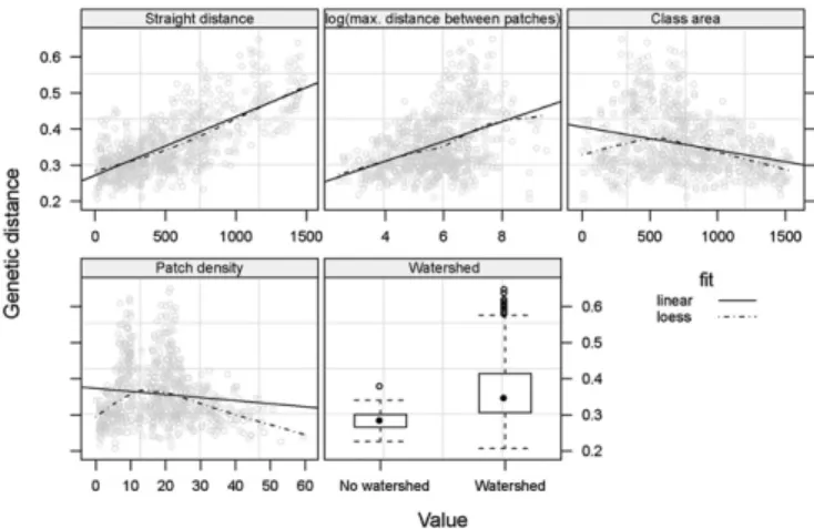
In the regression model, the main variables influencing genetic
distance were (i) the geographic distance, (ii) being located within
the same river basin, and (iii) three different metrics of habitat
fragmentation, namely the patch density [number of habitat patches
(i.e., tree cover
>20%) within the 0.2° pixels where landscape
friction is modeled], the class area [number of habitat pixels
(500
× 500 m)]), and the maximum distance between habitat
patches (Fig. 1). The findings were consistent with existing
knowl-edge of G. p. gambiensis ecology. For example, isolation by distance
is well known, as is the effect of watersheds on genetic distance,
even if the latter does not lead to complete isolation (
Fig. S4
) (11).
Human encroachment on tsetse habitat explains the positive effect
of habitat fragmentation on genetic distance: The further apart the
habitat patches, the more difficult for tsetse to disperse (Fig. 2) (17).
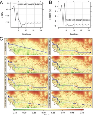
Identification of Tsetse Dispersal Paths.
Direct lines connecting the
sampled tsetse populations were initially used to model the genetic
distance against the environmental variables, thereby generating
the initial friction map. Subsequently, the average values for the
environmental variables were recalculated along the least-cost
paths based on the initial friction map (Fig. 3). To this end, a
transition matrix was computed from the friction map. To define
the connectedness between adjacent pixels, we used Rooks’
dis-tance as a neighborhood function, in which a given pixel is
considered to be connected to the four adjacent pixels. Then, the
least-cost paths between origin and destination points were
cal-culated, minimizing the mean values of friction for the pixels
crossed by the path. The new set of values of explanatory variables
extracted along this least-cost path was used to refit the regression
model. This procedure was repeated 20 times, and models fitted at
each iteration were compared with the Akaike information
crite-rion corrected for small sample size (AICc): The smaller, the
better. A large reduction of AICc was observed between the initial
model based on direct lines and the AICc-best model based on
least-cost paths:
Δ AICc = 18 (Fig. 3A). Thus, the regression
model based on least-cost paths (seventh iteration) was much
more plausible than the initial one. It also minimized the root
mean squared error (Fig. 3B).
Apart from the time between sampling events and the
geo-graphical distance, all variables retained in the AICc-best model
(coefficients in
Table S2
) were describing landscape connectivity
(i.e., landscape fragmentation metrics and the presence of a
watershed) (Fig. 2). There was a nonlinear relationship between
the density and area of habitat patches, as expected in a
fragmen-tation process (
Fig. S5
). Moreover, the interaction term between
these two variables was retained in the final model. The variables
informing on the composition and shape of the fragmented
land-scape and the geographic distance became more important in the
final model, whereas the importance of watersheds and
inter-actions was reduced (
Fig. S6
).
The use of least-cost distance confirmed the significant impact
of time between sampling dates on the genetic distance (
Table
S2
) (16). More importantly, it revealed the importance of
land-scape features related to functional connectivity (
Table S2
). The
iterative, least-cost-based analysis also improved the mapping of
ecological barriers to tsetse dispersal, with a more contrasted
picture of friction (Fig. 3C).
Distribution of G. p. gambiensis in the Study Area and Combination with Landscape Friction.
The habitat suitability for G. p. gambiensis
was estimated using a maximum entropy (MaxEnt) model and
mapped independently from landscape friction. Tsetse habitat
was positively associated to vegetation activity [i.e., normalized
difference vegetation index (NDVI)], average precipitations, and
humidity. Conversely, high values for temperature-related variables
Fig. 1. Shape and amplitude of the relationships between genetic distance, great-circle distance and environmental variables. CSE was calculated be-tween pairs of G. p. gambiensis populations (37 sampling sites listed inTable S1) and environmental variables are here extracted along the straight paths.
[land surface temperature (LST) and air temperature] led to a
low suitability index. Fig. 4 presents the respective contributions
and response curves for the different variables, the most important
being maximum LST and average precipitation. The predictive
power of the MaxEnt model was high, with an area under the
curve of 0.84 (Fig. 4). Moreover, the precision of MaxEnt
pre-dictions was the highest in the areas of interest (northern limit of
the tsetse belt), which was also the most intensively sampled area
(
Fig. S7
). Finally, we used a density-based clustering algorithm
applied to the MaxEnt output to identify eight clusters of suitable
habitat located at least 10 km apart from the main tsetse habitat.
Model Predictions and Consequences for Tsetse Control.
Fig. 5
pre-sents the eight potentially isolated clusters of tsetse habitat
lo-cated at the northern distribution limit of the G. p. gambiensis
belt in West Africa. The population with the highest predicted
genetic distance from the main tsetse belt (P
= 0.003) was close
to Thiès (Senegal). It is also the target of an ongoing eradication
campaign. For this population, genetic isolation was confirmed
by independent morphometric and genetic studies (9). Two other
clusters (6 and 8) with similar genetic distances from the tsetse
belt seemed to be isolated (P
= 0.001) and therefore represent
interesting potential targets for elimination efforts. Finally, two
other clusters could be isolated (2 and 7, P
< 0.05). Interestingly,
the situation in cluster 2 (Bijagos Islands in Guinea Bissau) is
reminiscent of the Loos Islands in Guinea (not visible in Fig. 5).
The tsetse populations in the Loos Islands were recently targeted
by an elimination program following the demonstration of their
isolation (8).
The present study provides information on potential targets
for tsetse elimination across a vast area. However, should one of
these populations be selected for an elimination program, more
comprehensive local studies would be needed, both to characterize
the exact extent and connectivity of the infested area and to confirm
its genetic isolation. These studies should include systematic
sam-pling of suitable habitats (18) and an independent genetic analysis
involving the target population and those closest to it (9).
Future Prospects.
Microsatellite genetic markers are available for
the most important tsetse species: Glossina fuscipes, Glossina
morsitans, Glossina pallidipes, and Glossina tachinoides.
Further-more, the recent sequencing of the full genome of G. morsitans
offers new prospects for either additional microsatellite markers or
other markers such as single-nucleotide polymorphisms (19).
Ap-plying the methodology described in this study to other tsetse
species and regions would provide decision makers with crucial
information on where control or eradication programs might be
more appropriate. Friction maps might also help in those
situa-tions where the populasitua-tions targeted for eradication are not isolated
(e.g., the Mouhoun River in Burkina Faso and northwestern
Ghana). In fact, artificial barriers to reinvasion such as traps
im-pregnated with insecticides (6) would be more effective if deployed
Fig. 2. Landscape fragmentation and river basins. Landscape fragmentation of G. p. gambiensis habitat based on a tree cover threshold of 20% (year 2000) (44) and related linear fragmentation indices. (A) Patch area. (B) Patch density. (C) Maximum distance of unsuitable area (or maximum distance between patches). (D) Locations of the tsetse sampling sites grouped by river basin (45).
Fig. 3. Least-cost distance vs. straight distance. (A) Observed changes in Akaike information criterion with small-sample size correction (AICc) and (B) rmse when replacing straight distance with least-cost distance computed from the friction raster, and iterating the process (x axis). (C) Changes in landscape genetic friction (colored map) and in least-cost distance (blue line) between two tsetse populations over the first seven iterations.
APPLIED
BIOLOGIC
AL
in high-friction areas. The use of such artificial barriers might
therefore enable sequential eradication programs, by dividing
the target populations into partially isolated subunits (20).
Fur-thermore, in those areas exposed to strong reinvasion pressure,
landscape friction analysis could guide the adoption of alternative
strategies (e.g., reduction of tsetse densities below the threshold
of disease transmission), thus preventing major economic losses
due to unsuccessful eradication attempts.
Finally, identifying natural barriers to dispersal and quantifying
their environmental determinants might help to manage other
pests, or conversely it could be used to improve the conservation
of endangered species occurring as metapopulations (21).
In-deed, locating genetic corridors across high-friction landscapes is
becoming crucial for the conservation of natural populations in a
context of increasing fragmentation of ecosystems (12).
Methods
Genetic Analysis. We inferred tsetse dispersal using the CSE calculated be-tween 37 populations of G. p. gambiensis from West Africa. Samples were collected along the northern limit of the distribution, where tsetse habitat is most fragmented (22) (Table S3). Most populations (24 out of 37) were specifically sampled for this study using biconical traps (1–11 traps by site). Traps were set at∼100-m intervals for a maximum period of 1 wk and with a maximum distance of 1 km between first and last traps (10). We also in-cluded in the analysis 13 previously sampled populations (9, 10). The geo-graphical coordinates and data collection dates are presented inTable S3. Each population was sampled once.
In total, 1,158 flies were genotyped at seven loci following a previously described protocol (16). All genotyping was handled or supervised by the same person (S.R.), thus ensuring optimal calibration of allele sizes across
subsamples. Males were coded as homozygous at X-linked loci. Overall, 61% of the flies were females, which are more informative given that four out of the seven loci are X-linked. Details on the genotyping procedure and the loci selected are presented inDetails on the Genetic Analysis, together with tests of linkage disequilibrium and departure from Hardy–Weinberg (HW) equilibrium. Three different genetic distances were initially explored: Wright’s fixation index FST(23), CSE (24), and Bowcock et al.’s shared allelic distance (25). After
an exploratory data analysis, CSE was selected, because it behaves better in case of missing data and is more appropriate for measuring relative distances between pairs of populations (26–28). We detail how CSE was calculated in
Details on the Genetic Analysis.
Environmental Datasets for the Analysis of Genetic Distance. First, we explored the relationship between CSE and expert-based land-cover permeability scores (Table S1andFig. S1). Because of the failure of the latter to predict observed genetic distances, a range of spatially explicit environmental datasets selected based on the ecology of G. p. gambiensis were explored as explanatory variables. We considered climate (temperature and rainfall), land cover, human and cattle population, and topography (average slope and elevation change) (Figs. S2andS3andEnvironmental Variables and Relationship with the Genetic Distance). We also considered hydrological features (river basins) and habitat fragmentation metrics derived from Moderate Resolution Imaging Spectroradiometer (MODIS) tree cover (i.e., the area and density of patches of suitable habitat and the maximum dis-tance between patches of suitable habitat) (Fig. 2,Fig. S4, and Environ-mental Variables and Relationship with the Genetic Distance). Considering the collection dates of the entomological data (2007–2010), and given the studied genetic markers, we focused on environmental datasets collected after 2000. For all gridded environmental datasets, average values were calculated along each line connecting tsetse sampling sites pairwise. Principal Fig. 4. Distribution of G. p. gambiensis in West Africa. (A) Mean habitat
suitability index predicted by a MaxEnt model. The index varies between 0 (less suitable, red scale) and 1 (highly suitable, green scale). (B) Contribu-tion of variables to the suitability index by decreasing importance (95% confidence interval in red and individual values in blue). lst_max, maximum land surface temperature (MODIS); lst_min, minimum land surface tempera-ture (MODIS); mir_max, maximum mid-infrared reflectance (MODIS); mir_min, minimum mid-infrared reflectance; ndvi_max, maximum normalized differ-ence vegetation index (MODIS); ndvi_min, minimum normalized differdiffer-ence vegetation index (MODIS); prec_mean, mean yearly rainfalls (WorldClim grid); t_mean, mean annual temperature (WorldClim grid). (C and D) Response curves of the most contributing variables (lst_max and prec_mean, respectively). (E) Area under the curve for the average MaxEnt model (in red) and the 45 submodels (in blue) (seeDetails on the MaxEnt Modelfor details).
Fig. 5. Isolated patches of suitable habitat for G. p. gambiensis. (A) Land-scape friction is the colored background, and habitat patches are delimited with blue contours. (B) The main tsetse belt predicted by MaxEnt for a sensitivity of 0.90 is in gray and habitat patches are shown as filled, red shapes. Contours and shapes of isolated patches were defined as 5-km radius buffers around pixels of habitat patches. The genetic distance of these patches to the main tsetse belt (reddish scale) was predicted by the AICc-best regression model along least-cost paths. Asterisks after cluster numbers represent the P values for the friction between the patches and the general habitat: (***) P= 10−3, (**) 10−3≤ P < 10−2, (*) 10−2≤ P < 5 10−2.
components analysis was used to identify the most correlated variables. When strong correlations were found (jrj > 0.8), one of the variables was discarded, and the one with the most straightforward or acknowledged effect on the genetic distance was retained (Environmental Variables and Relationship with the Genetic Distance). To assess the shape and strength of the relationship between genetic distance and predictors, scatterplots were drawn with superimposed linear and loess-smoothed fits (Fig. 1 andFig. S4). To account for the nonlinear fragmentation process (Fig. S5), the patch density was discretized into three categories (low, medium, and high). Ad-ditional data on this exploration phase and on how the data were prepared for the model are presented inEnvironmental Variables and Relationship with the Genetic Distance.
Linear Regression Model of the Genetic Distance. The goal was to find the best environmental predictors of the genetic distance between pairs of tsetse fly populations. We used a linear regression model fitted with generalized least squares (GLS) (29), having the genetic distance (CSE) as the response, and the selected environmental variables as the predictors. The time elapsed be-tween population sampling was forced into the models to control for pos-sible genetic drift. To account for pospos-sible autocorrelation, we clustered tsetse populations according to the geographic distance. Hierarchical as-cending clustering (Ward method) was used to form partitions of various sizes (from 1 to 19 clusters) based on the Euclidian distance between pairs of populations. Cluster membership was then used to define the grouping structure in the GLS model (30). We selected the eight-cluster partition for which AICc was the lowest with the full GLS model (with all fixed effects) (31). Preliminary analyses revealed that model residuals increased with the fitted genetic distance. To account for this heteroscedasticity, we modeled residuals variance with a power function of the fitted values. Model good-ness of fit was assessed using various indicators, including the proportion of variance explained by the fixed effects, quantile–quantile plots of residuals, and the detection of influential observations for GLS coefficients.
Finally, we selected the AICc-best model among all possible submodels in which were forced the Euclidian distance between tsetse populations and the time elapsed between population sampling. Regarding model validation, model selection with Akaike information criteria is formally equivalent to model cross-validation (32). We checked our results with the asymptotically equivalent leave-one-cluster-out cross-validation (CLCV). To do so, we fitted the model to the data with all of the cluster-based groups of distances but one, and predicted the genetic distance with this model for the populations belonging to the left-out group. Prediction errors were then summed for this group, and the process was iterated for all groups. The averaged pre-diction error was then used as the CLCV indicator to compare the 10 AICc-best models. The first four models were very close in terms of AICc and CLCV, and more generally there was a good agreement between AICc and CLCV (Spearman’s rank correlation of 0.65, P = 0.02).
To build the friction maps, the AICc-best model was used to predict the genetic distance at each pixel location for the different predictors, setting at 0 both the time elapsed between population sampling and the geographical distance.
Building the Least-Cost Paths. The first iteration of the least-cost paths was based on the initial friction map, as built using the direct paths. Least-cost distances between origin and destination points were calculated using the functions available in the raster and gdistance packages for R (33, 34). Then, averages for all environmental variables were recalculated along the least-cost paths, and Euclidian distances were replaced by the least-least-cost distances. We subsequently refitted the full model and we selected the AICc-best submodel. The latter was then used to predict the friction across the study region. Finally, we recomputed the least-cost distances based on the updated friction map and iterated this process until the AICc of the best model was stabilized (Fig. 3A). Fig. 3C presents the initial friction and its changes for the first seven iterations.Table S2andFig. S6present the coefficients of the AICc-best model used to build the final friction map and to predict the genetic distance between the potentially isolated tsetse populations asso-ciated with the eight habitat clusters (Fig. 5). The dataset including all en-vironmental parameters and the genetic distances between pairs of populations is available asDataset S1.
Tsetse Distribution Model. The entomological data used for the regional distribution model of G. p. gambiensis originated from recent baseline surveys for tsetse eradication projects in West Africa: 2007–2008 in Senegal (18), 2008– 2009 in Ghana, and 2007–2012 in Burkina Faso (35). Unbaited biconical traps were used in all surveys (36). For the present analysis, only presence/absence
data were used. Absence data were filtered by the duration of trapping (≥3 d), and absence data within 5 km from a presence data were discarded. Presence and absence data were also filtered to keep only one presence or absence point within a radius of 5 km. From the initial 2,853 presence and 6,088 absence records, 450 and 516 data points, respectively, were finally retained.
Regarding environmental data used to predict habitat suitability, time series of high-spatial-resolution remote sensing data (1 km) were down-loaded, cleaned, and summarized to build relevant environmental and cli-matic covariates. We combined 11 y of MODIS vegetation and thermal products (January 2003–December 2013). Eight-day composite daytime (DLST) and nighttime land surface temperature (NLST) were extracted from MOD11A2/MYD11A2 temperature and emissivity MODIS products. DLST and NLST were used as proxies for both soil and air temperature, which play an important role in shaping tsetse habitat. Low-quality pixels were removed from the raw data using the quality assessment layer and outliers were fil-tered using a variant of the boxplot algorithm (37). Vegetation indices at 1 km of spatial resolution and with temporal resolution of 16 d (MOD13A2/ MYD13A2) were also downloaded and processed using the quality assess-ment layer. In particular, the NDVI and middle infrared (MIR) reflectance were selected to describe the vegetation and soil condition in the study area. Temperature and precipitation from WorldClim were also used (38).
A MaxEnt model was used to estimate a habitat suitability index for G. p. gambiensis in the study area (39). The logistic output from this method is a suitability index that ranges between 0 (less suitable habitat) and 1 (highly suitable habitat). The threshold for presence was set to allow a 90% sensitivity (40). Details on the parameterization of MaxEnt and the selection of pseu-doabsences are available inDetails on the MaxEnt Model.
Identification of Isolated Patches. To identify the connected patches from the MaxEnt output, we used the function ConnCompLabel in the SDMTools package (41). Then, we used a clustering algorithm to detect clusters of pixels based on their geographical proximity. To this end, we used the function dbscan from the eponymous R package (42). We withdrew isolated pixels as well as those belonging to small clusters (fewer than 20 pixels). Then, we computed the minimum distance between the (centroids of) cluster pixels and those from the general population. We discarded clusters located at less than 10 km from the main tsetse belt because they were unlikely to be genetically isolated from it, and these pixels were thereafter considered as part of the main tsetse belt. Then, we grouped together clusters that were geographically close to each other using a hierarchical ascending classification procedure, with the so-called simple (neighbor-joining) algorithm. At the end of this step, nine clusters were left. One of them was discarded because it was cut by the eastern limit of the analysis window. Finally, we computed the predicted least-cost distance between the clusters and the main tsetse belt using the AICc-best model and the friction raster formerly estimated (Fig. 5 and Table S2). In this sample of eight habitat patches, the correlation of geographic and genetic distances was not significant (Spearman’s rank correlation of 0.43, P = 0.30). To test the sig-nificance of the isolation of these clusters, a statistical test was built whereby for each cluster the genetic distance to the main tsetse belt was compared with those between 999 pairs of points randomly generated within the main belt, with the same geographical distance between them as between the patch and the general population (minimum P= 0.001). All genetic distances between pairs of points were computed with the procedure previously de-scribed, using the AICc-best model and the friction raster formerly esti-mated. All analyses were conducted using R software (43).
ACKNOWLEDGMENTS. The joint Food and Agriculture Organization of the United Nations/International Atomic Energy Agency (IAEA) Programme of Nuclear Techniques in Food and Agriculture and the IAEA’s Department of Technical Cooperation funded fly collections and genotyping. The work of J.B. was conducted within the research project“Integrated Vector Manage-ment: innovating to improve control and reduce environmental impacts” of Institut Carnot Santé Animale excellence network. FAO contribution to this study was also provided in the framework of the Programme Against African Trypanosomosis; in particular, financial support was provided by the Govern-ment of Italy through the FAO project“Improving food security in sub-Saharan Africa by supporting the progressive reduction of tsetse-transmitted trypano-somosis in the framework of NEPAD” (GTFS/RAF/474/ITA). The work of T.D.M. and P.S. was conducted within Maladies à vecteurs en Afrique de l’Ouest, Burkina Faso. This study was also partially funded by European Union Grant FP7-261504 EDENext and is catalogued by the EDENext Steering Committee as EDENext339 (www.edenext.eu).
APPLIED
BIOLOGIC
AL
1. WHO (2013) Control and Surveillance of Human African Trypanosomiasis (World Health Organization, Geneva).
2. Swallow BM, ed (2000) Impacts of Trypanosomiasis on African Agriculture (FAO, Rome).
3. Alsan M (2015) The effect of the tsetse fly on African development. Am Econ Rev 105(1):382–410.
4. Bouyer F, et al. (2014) Ex-ante benefit-cost analysis of the elimination of a Glossina palpalis gambiensis population in the Niayes of Senegal. PLoS Negl Trop Dis 8(8): e3112.
5. Vreysen MJB, Seck MT, Sall B, Bouyer J (2013) Tsetse flies: Their biology and control using area-wide integrated pest management approaches. J Invertebr Pathol 112(Suppl): S15–S25.
6. Kgori PM, Modo S, Torr SJ (2006) The use of aerial spraying to eliminate tsetse from the Okavango Delta of Botswana. Acta Trop 99(2-3):184–199.
7. Vreysen MJB, et al. (2000) Glossina austeni (Diptera: Glossinidae) eradicated on the island of Unguja, Zanzibar, using the sterile insect technique. J Econ Entomol 93(1): 123–135.
8. Solano P, et al. (2009) The population structure of Glossina palpalis gambiensis from island and continental locations in Coastal Guinea. PLoS Negl Trop Dis 3(3):e392. 9. Solano P, et al. (2010) Population genetics as a tool to select tsetse control strategies:
Suppression or eradication of Glossina palpalis gambiensis in the Niayes of Senegal. PLoS Negl Trop Dis 4(5):e692.
10. Koné N, et al. (2011) Contrasting population structures of two vectors of African trypanosomoses in Burkina Faso: Consequences for control. PLoS Negl Trop Dis 5(6): e1217.
11. Vreysen MJ, et al. (2013) Release-recapture studies confirm dispersal of Glossina palpalis gambiensis between river basins in Mali. PLoS Negl Trop Dis 7(4):e2022. 12. Spear SF, Balkenhol N, Fortin M-J, McRae BH, Scribner K (2010) Use of resistance
surfaces for landscape genetic studies: Considerations for parameterization and analysis. Mol Ecol 19(17):3576–3591.
13. Zeller KA, McGarigal K, Whiteley AR (2012) Estimating landscape resistance to movement: A review. Landscape Ecol 27(6):777–797.
14. Peterman WE, Connette GM, Semlitsch RD, Eggert LS (2014) Ecological resistance surfaces predict fine-scale genetic differentiation in a terrestrial woodland salaman-der. Mol Ecol 23(10):2402–2413.
15. Bouyer J, et al. (2009) Population sizes and dispersal pattern of tsetse flies: Rolling on the river? Mol Ecol 18(13):2787–2797.
16. De Meeûs T, Ravel S, Rayaisse J-B, Courtin F, Solano P (2012) Understanding local population genetics of tsetse: The case of an isolated population of Glossina palpalis gambiensis in Burkina Faso. Infect Genet Evol 12(6):1229–1234.
17. Dicko AH, et al. (2014) Using species distribution models to optimize vector control in the framework of the tsetse eradication campaign in Senegal. Proc Natl Acad Sci USA 111(28):10149–10154.
18. Bouyer J, Seck MT, Sall B, Guerrini L, Vreysen MJB (2010) Stratified entomological sampling in preparation of an area-wide integrated pest management programme: The example of Glossina palpalis gambiensis in the Niayes of Senegal. J Med Entomol 47(4):543–552.
19. International Glossina Genome Initiative (2014) Genome sequence of the tsetse fly (Glossina morsitans): Vector of African trypanosomiasis. Science 344(6182):380–386. 20. Hendrichs J, Vreysen MJB, Enkerlin WR, Cayol JP (2005) Strategic options in using
sterile insects for area-wide integrated pest management. Sterile Insect Technique, eds Dyck VA, Hendrichs J, Robinson AS (Springer, Dordrecht, The Netherlands), pp 563–600.
21. Hanski I, Ovaskainen O (2000) The metapopulation capacity of a fragmented land-scape. Nature 404(6779):755–758.
22. Guerrini L, Bord JP, Ducheyne E, Bouyer J (2008) Fragmentation analysis for prediction of suitable habitat for vectors: Example of riverine tsetse flies in Burkina Faso. J Med Entomol 45(6):1180–1186.
23. Wright S (1965) The interpretation of population structure by F-statistics with special regard to system of mating. Evolution 19(3):395–420.
24. Cavalli-Sforza LL, Edwards AWF (1967) Phylogenetic analysis. Models and estimation procedures. Am J Hum Genet 19(3 Pt 1):233–257.
25. Bowcock AM, et al. (1994) High resolution of human evolutionary trees with poly-morphic microsatellites. Nature 368(6470):455–457.
26. de Meeûs T, et al. (2007) Population genetics and molecular epidemiology or how to “débusquer la bête”. Infect Genet Evol 7(2):308–332.
27. Takezaki N, Nei M (1996) Genetic distances and reconstruction of phylogenetic trees from microsatellite DNA. Genetics 144(1):389–399.
28. Kalinowski ST (2002) Evolutionary and statistical properties of three genetic distances. Mol Ecol 11(8):1263–1273.
29. Laird NM, Ware JH (1982) Random-effects models for longitudinal data. Biometrics 38(4):963–974.
30. Dormann CF, et al. (2007) Methods to account for spatial autocorrelation in the analysis of species distributional data: A review. Ecography 30(5):609–628. 31. Hurvich CM, Tsai C-L (1995) Model selection for extended quasi-likelihood models in
small samples. Biometrics 51(3):1077–1084.
32. Fang Y (2011) Asymptotic equivalence between cross-validations and Akaike In-formation Criteria in mixed-effects models. J Data Sci 9:15–21.
33. Hijmans RJ (2015) raster: Geographic data analysis and modeling, R package version 2.4-15. Available at https://cran.r-project.org/web/packages/raster/index.html. 34. van Etten J (2012) gdistance: Distances and routes on geographical grids, R package
version 1:1-4. Available at CRAN.R-project.org/package=gdistance.
35. Dicko AH, et al. (2015) A spatio-temporal model of African animal trypanosomosis risk. PLoS Negl Trop Dis 9(7):e0003921.
36. Challier A, Laveissière C (1973) Un nouveau piège pour la capture des glossines (Glossina: Diptera, Muscidae): Description et essais sur le terrain. Cah ORSTOM sér Ent Méd Parasitol 10(4):251–262.
37. Neteler M (2010) Estimating daily land surface temperatures in mountainous envi-ronments by reconstructed MODIS LST data. Remote Sens 2(1):333–351.
38. Hijmans R, Cameron S, Parra J, Jones P, Jarvis A (2005) Very high resolution in-terpolated climate surfaces for global land areas. Int J Climatol 25:1965–1978. 39. Elith J, et al. (2011) A statistical explanation of MaxEnt for ecologists. Divers Distrib
17(1):43–57.
40. Liu C, Berry PM, Dawson TP, Pearson RG (2005) Selecting thresholds of occurrence in the prediction of species distributions. Ecography 28(3):385–393.
41. VanDerWal J, Falconi L, Januchowski S, Shoo L, Storlie C (2014) SDMTools: Species dis-tribution modelling tools: Tools for processing data associated with species disdis-tribution modelling exercises, R package version 1.1-221. Available at https://cran.r-project.org/web/ packages/SDMTools/index.html.
42. Hahsler M (2015) dbscan: Density Based Clustering of Applications with Noise (DBSCAN), R package version 0.9-1. Available at https://cran.r-project.org/web/packages/ dbscan/index.html.
43. R Core Team (2015) R: A language and environment for statistical computing (R Foundation for Statistical Computing, Vienna). Available at www.R-project.org. 44. Hansen M, et al. (2003) Global percent tree cover at a spatial resolution of 500 meters:
First results of the MODIS vegetation continuous fields algorithm. Earth Interact 7(10):1–15.
45. Lehner B, Verdin K, Jarvis A (2008) New global hydrography derived from spaceborne elevation data. Eos 89(10):93–94.
46. Solano P, Duvallet G, Dumas V, Cuisance D, Cuny G (1997) Microsatellite markers for genetic population studies in Glossina palpalis (Diptera: Glossinidae). Acta Trop 65(3): 175–180.
47. Luna C, et al. (2001) Microsatellite polymorphism in tsetse flies (Diptera: Glossinidae). J Med Entomol 38(3):376–381.
48. Baker MD, Krafsur ES (2001) Identification and properties of microsatellite markers in tsetse flies Glossina morsitans sensu lato (Diptera: Glossinidae). Mol Ecol Notes 1(4): 234–236.
49. De Meeûs T, Guégan JF, Teriokhin AT (2009) MultiTest V.1.2, a program to binomially combine independent tests and performance comparison with other related methods on proportional data. BMC Bioinformatics 10:443.
50. Goudet J (1995) FSTAT (v. 1.2): A computer program to calculate F-statistics. J Hered 86(6):485–486.
51. Van Oosterhout C, Hutchinson WF, Wills DPM, Shipley P (2004) MICRO-CHECKER: Software for identifying and correcting genotyping errors in microsatellite data. Mol Ecol Notes 4(3):535–538.
52. Brookfield JFY (1996) A simple new method for estimating null allele frequency from heterozygote deficiency. Mol Ecol 5(3):453–455.
53. Dieringer D, Schlötterer C (2003) Microsatellite analyser (MSA): A platform independent analysis tool for large microsatellite data sets. Mol Ecol Notes 3(1):167–169. 54. Coombs JA, Letcher BH, Nislow KH (2008) create: A software to create input files from
diploid genotypic data for 52 genetic software programs. Mol Ecol Resour 8(3): 578–580.
55. Mayaux P, Bartholomé E, Fritz S, Belward A (2004) A new land-cover map of Africa for the year 2000. J Biogeogr 31(6):861–877.
56. Arino O, et al. (2007) GlobCover: ESA service for global land cover from MERIS. IEEE International Geoscience and Remote Sensing Symposium, 2007 (IEEE, New York), pp 2412–2415.
57. Van Zyl JJ (2001) The Shuttle Radar Topography Mission (SRTM): A breakthrough in remote sensing of topography. Acta Astronaut 48(5):559–565.
58. Keyghobadi N, Roland J, Strobeck C (1999) Influence of landscape on the population genetic structure of the alpine butterfly parnassius smintheus (Papilionidae). Mol Ecol 8(9):1481–1495.
59. Balk D, Yetman G (2004) The Global Distribution of Population: Evaluating the Gains in Resolution Refinement (Center for International Earth Science Information Net-work, Columbia Univ, New York).
60. Center for International Earth Science Information Network, Columbia University International Food Policy Research Institute, the World Bank, and Centro Inter-nacional de Agricultura Tropical (2004) Global Rural-Urban Mapping Project (GRUMP): Urban/Rural Population Grids (Center for International Earth Science Information Net-work, Columbia Univ, Palisades, NY).
61. Dobson J, Bright E, Coleman P, Durfee R, Worley B (2000) LandScan: A global population database for estimating populations at risk. Photogramm Eng Remote Sensing 66(7): 849–857.
62. Wint W, Robinson TP (2007) Gridded Livestock of the World 2007 (FAO, Rome). 63. Dudík M, Phillips SJ, Schapire RE (2005) Correcting sample selection bias in maximum
entropy density estimation. Advances in Neural Information Processing Systems (MIT Press, Cambridge, MA), pp 323–330.
64. Phillips SJ, et al. (2009) Sample selection bias and presence-only distribution models: Implications for background and pseudo-absence data. Ecol Appl 19(1):181–197. 65. Zomer RJ, Trabucco A, Bossio DA, Verchot LV (2008) Climate change mitigation: A
spatial analysis of global land suitability for clean development mechanism affores-tation and reforesaffores-tation. Agric Ecosyst Environ 126(1):67–80.