Adaptive Optics for High Energy Laser Systems
by
Joseph Edward Wall,
mI
B.S., Electrical Engineering, Tulane University, (1992)
SUBMITTED TO THE DEPARTMENT OF
ELECTRICAL ENGINEERING AND COMPUTER SCIENCE
IN PARTIAL FULFILLMENT OF THE REQUIREMENTS FOR THE DEGREE OF
MASTER OF SCIENCE
IN ELECTRICAL ENGINEERING AND COMPUTER SCIENCE
at the
MASSACHUSETTS INSTITUTE OF TECHNOLOGY
May 1994
© Joseph E. Wall, III
Signature of Author
0(
'
Deparmnent of Electrical Engineering
and Comnuter Science, May 1994
Certified by
"I
'
Dr. Brent Appleby
Technical Supervisor
Charles Stark Draner Laboratory
Certified by
Dr. Michael Athans
Professor of Systems Science and Engineering
Deparm t of Electieangineering
and Computer Science
\
I Hl,
,
n~ Thesis Supervisor
Accepted by
X
~
'-
Frederic
k.-IMorgenthaler
ChairnG,- Deponet
Graduate Committee
Department f Electrical Engineering and Computer Science
Adaptive Optics for High Energy Laser Systems
by
Joseph Edward Wall, III
Submitted to the Department of Electrical Engineering and Computer Science on May 30, 1994 in Partial Fulfillment of the Requirements for
the Degree of Master of Science in Electrical Engineering and Computer Science
ABSTRACT
High-energy laser propagation in the atmosphere requires consideration of self-induced
beam expansion due to thermal blooming and random distortion due to atmospheric
turbulence. Thermal blooming is a result of interaction between the laser radiation and the propagation path. A small portion of the laser energy is absorbed by the atmosphere. This energy heats the air causing it to expand and form a distributed thermal lens along the path. The refractive index of the medium is decreased in the region of the beam where heating is
the greatest, causing the beam to spread. Atmospheric turbulence is caused by random
naturally occurring temperature gradients in the atmosphere.
This research focuses on the design of beam control systems for high-energy lasers. In
particular, it compares traditional phase conjugation and open loop techniques to a
model-based optimal correction technique which modifies the laser power and focal length. For
light thermal blooming, phase conjugation is seen to be a reasonable control strategy.
However, as the level of thermal blooming increases, phase conjugation performs
increasingly worse. For moderate to heavy thermal blooming scenarios, the new technique is shown to increase peak intensity on target up to 50% more than traditional compensation
methods. Additionally, the optimal correction technique is insensitive to errors in the
model parameters. The system under consideration is a ground-based continuous wave
laser operating in an environment with wind. It is assumed that a tracking system provides target position and velocity information. A reflection of the laser wavefront off the target is useful, but not required.
Thesis Supervisor: Dr. Michael Athans
Title: Professor of Systems Science and Engineering
Technical Supervisor: Dr. Brent Appleby
Acknowledgments
I would like to thank The Charles Stark Draper Laboratory for providing me with the
opportunity to pursue my graduate studies at MIT. I am especially grateful to my
supervisor at Draper, Dr. Brent Appleby, for his continuous assistance with all aspects of
my research.
Additionally, I would like to thank Greg Cappiello for his assistance with the optical part of
the project, Dr. John Dowdle for his overall guidance, and Professor Michael Athans for
his inspiring courses and insightful suggestions for this thesis.
This thesis was prepared at The Charles Stark Draper Laboratory, Inc., under Independent
Research and Development Project No. 529: Adaptive Optics for Beam Control in an
Unstable Medium. Draper Laboratory's financial support under this project was greatly
appreciated.
Publication of this thesis does not constitute approval by the Draper Laboratory or the
Massachusetts Institute of Technology of the findings or conclusions contained herein. It
is published for the exchange and stimulation of ideas.
I hereby assign my copyright of this thesis to The Charles Stark Draper Laboratory, Inc.,
Cambridge, Massachusetts.
Permission is hereby granted by The Charles Stark Draper Laboratory, Inc., to the
Table of Contents
List of Tables ...
11
List of Figures ...
13
1
Introduction
...
171.1
Typical High Energy Laser Platform ...
18
1.2 High Energy Laser Issues ... 20
1.3 Project Purpose ... ... ... 1
1.4 Phase Conjugation Overview ... 22
1.5
Thesis Contributions ...
23
1.6
Thesis Outline ...
24
2
Mathematical Foundation of Thermal Blooming ... 27
2.1 Analytic Derivation of Thermal Blooming Equations ... 28
2.2 Approximations to Steady State Thermal Blooming ... 29
2.3 Relationship Between Phase Error and Intensity ... 32
2.4 Introduction to Zernike Polynomials ... 35
2.5
Summary ...
35
3
Thermal Blooming Model ...
37
3. 1 Thermal Blooming Model Parameters ... 37
3.2
Peak Intensity ...
...
...
...
9
3.3
Critical Power ...
41
3.4
Dispersive
Effects
.
.
...
... 42
3.4.1 Random Linear Effects ... 42
3.4.2 Deterministic Nonlinear Effects ...
43
3.4.3 Heating Phase ...
44
3.5
Parameterization of Aberrated Beam
..
... 46
3.5.1 Focus ...
48
3.5.2 Astigmatism
... . ... ... ... 48
3.5.3 Coma ...
49
3.5.4 Spherical ...
50
3.7
Summary ...
...
.
52
4
Atmospheric Turbulence Model ...
53
4.1 Turbulence Model Parameters ... 53
4.2 Zernike Coefficient Modeling ... 54
4.2.1 Power Spectral Density ...
55
55...
4.2.2 Power Spectral Density Approximation ... 574.2.3 Transfer Function Gain ...
59
59...
4.3
Simulations ...
61
4.4
Covariance of Primary Modes ...
...
66
4.5
Summary
...
...
68
5
Optimal Atmospheric Correction ...
...
69
5.1 Control Strategies ... 70
5.1.1 Open Loop ... 70
5.1.2 Phase Conjugation ...
70
5.1.3 Optimal Focal Length ... ... 1...71
5.1.4 Optimal Focal Length with Optimal Power ... 72
5.2
Sim ulations ...
... 73
5.2. 1 Light Thermal Blooming ... 73
5.2.2 Moderate Thermal Blooming ...
76
5.2.3 Heavy Thermal Blooming ...
79
5.3
Summary ...
82
6
Parameter Sensitivity and Estimation ...
85
6.1
Parameter Sensitivity ...
86
6.2
Extended Kalman Filter Design ...
88
6.2.1 Basic Equations ...
88
6.2.2 Implementation ...
91
6.3
Simulations ...
93
6.4
Summary ...
103
7
Realistic Thermal Blooming Correction ... 105
7.1 Parameter Uncertainty Models ... 106
7.1.1 Atmospheric Constants .
...
106
7.1.3 Wind ...
106
7.2
Simulations ...
107
7.2.1 Light Thermal Blooming ...
... 107
7.2.2 Moderate Thermal Blooming ... ... 1
7.2.3 Heavy Thermal Blooming ... ... ... 115
7.3
Summary ...
...
... l 19
8
Conclusions ... ...
121
8.1 Conclusions ... 121
8.2
Recommendations ...
123
A
Zernike Polynom ials ...125
B
Parameter Sensitivity ...
...
133
List of Tables
3.1 Thermal Blooming Model Parameters ... ...38
4.1
Atmospheric Turbulence Model Parameters ...
54
4.2
h-Functions ...
56
4.3 Atmospheric Turbulence Scaled Corner Frequencies (Hertz) ... 58
4.4 Zernike Mode Variance Relative to , ... 6 1 A. 1 Zernike Polynomial Functions ... 126
List of Figures
1.1
Typical High Energy Laser Platform ...
20
1.2 Effect of Thermal Blooming on Power-Intensity Curve ... 2 1 1.3 Phase Conjugation Overview ... 23
2.1 Wavefront and Equal Intensity Contours for a Thermally Bloomed Wave ... 3 2 2.2 Coordinate System for Intensity Equations ... 3 3
2.3
Strehl Ratio as a Function of Wavefront Error ... 35
3.1
Effects of Diffraction and Thermal Blooming on Beam Spreading ...39
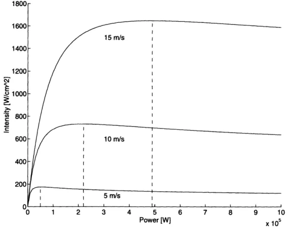
3.2 Intensity as a Function of Laser Power for Various Wind Speeds ... 42
3.3
Ray Diagram for Focus Aberration ...
48
3.4 Ray Diagram for Astigmatism Aberration ... 49
3.5 Ray Diagram for Coma Aberration ... 49
3.6 Ray Diagram for Spherical Aberration ... 50
3.7 Typical Wavefront for Light Thermal Blooming ... ... .51
3.8 Typical Wavefront for Heavy Thermal Blooming ... 5 1 4.1 Model for Zernike Turbulence Coefficient ... 55
4.2 Wavefront Distortion Due to Turbulence, Stationary Target Light Wind ... 62
4.3 Wavefront Distortion Due to Turbulence, Moving Target Moderate Wind ... 62
4.4 RMS Zernike Coefficient Values Corresponding to Figure 4.2 ... 63
4.5 RMS Zernike Coefficient Values Corresponding to Figure 4.3 ... 63
4.6
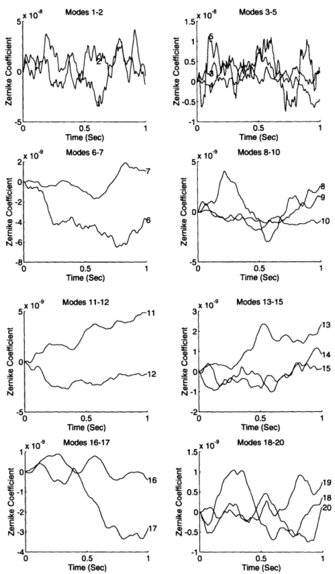
Zernike Coefficient Time History Corresponding to Figure 4.2 ... 64
4.7
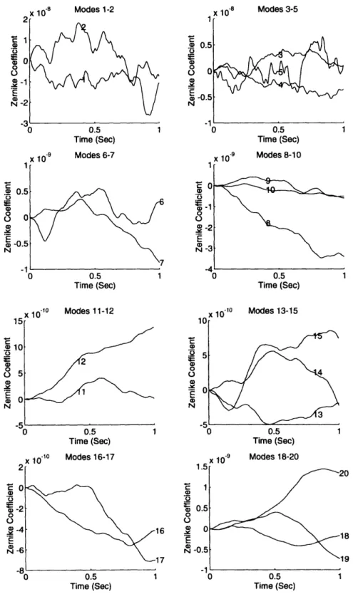
Zernike Coefficient Time History Corresponding to Figure 4.3 ... 65
5.1 Intensity as a Function of Focal Length ... 7 2
5.2
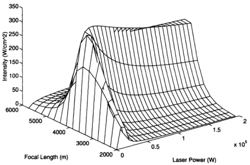
Intensity as a Function of Focal Length and Laser Power ... 73
5.3 Target Route for Light Thermal Blooming Scenario ... ... 74
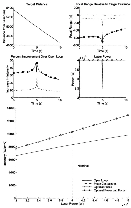
5.4
Performance Comparison for Light Thermal Blooming ...
75...7
5
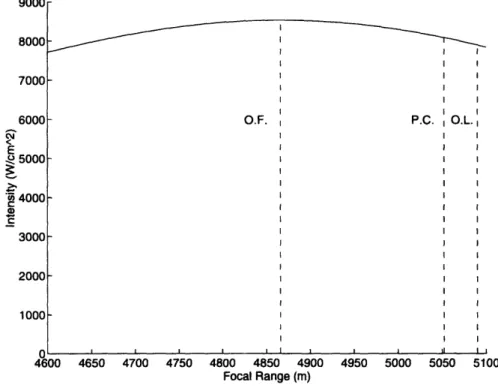
5.5 Intensity as a Function of Focal Length for Light Thermal Blooming Indicating Open Loop, Phase Conjugate, and Optimal Focus Focal Ranges ... 765.7 Performance Comparison for Moderate Thermal Blooming ... 78
5.8 Intensity as a Function of Focal Length for Moderate Thermal Blooming Indicating Open Loop, Phase Conjugate, and Optimal Focus Focal Ranges ... 79
5.9 Target Route for Heavy Thermal Blooming Scenarios ... 80
5.10
Performance Comparison for Heavy Thermal Blooming ... 81
5.11 Intensity as a Function of Focal Length for Heavy Thermal Blooming Indicating Open Loop, Phase Conjugate, and Optimal Focus Focal Ranges ... 82
6.1 Sensitivity to Refractive Index ... 8...87
6.2
Sensitivity to Transverse Wind Velocity ...
88
6.3
Kalman Filter Performance with Parameters Known Exactly ... 94
6.4
Kalman Filter Performance with Maximum Parameter Error of 2.5% ...
95
6.5
Kalman Filter Performance with Maximum Parameter Error of 5% ...
95
6.6 Kalman Filter Performance with Maximum Parameter Error of 10% ... 96
6.7 RMS Wind Estimate Error as a Function of Target Velocity Error ... 97
6.8
RMS Wind Estimate Error as a Function of Target Distance Error ... 97
6.9 Estimation Error Statistics for Light Thermal Blooming Simulations ... 99
6.10 Estimation Error Statistics for Light Thermal Blooming Simulations ... 100
6.11 Return Wavefront Zernike Coefficients as a Function of Wind Speed ... 101
6.12 Estimation Error Statistics for Heavy Thermal Blooming Simulations ... 102
7.1
Performance Comparison for Light Thermal Blooming ... 108
7.2 Estimator Performance for Light Thermal Blooming ... 109
7.3 Performance Comparison for Light Thermal Blooming with Parameter Errors... 110
7.4 Estimator Performance for Light Thermal Blooming with Parameter Errors ... I 1 7.5 Performance Comparison for Moderate Thermal Blooming ... 112
7.6 Estimator Performance for Moderate Thermal Blooming ... 113
7.7 Performance Comparison for Moderate Thermal Blooming with Parameter
Errors
...
114
7.8 Estimator Performance for Moderate Thermal Blooming with Parameter Errors . 115 7.9 Performance Comparison for Heavy Thermal Blooming ... 116
7.10 Estimator Performance for Heavy Thermal Blooming ... 117... 117
7.11 Performance Comparison for Heavy Thermal Blooming with Parameter Errors.. 1 18 7.12 Estimator Performance for Heavy Thermal Blooming with Parameter Errors ... 119
A.
Zernike Polynomial Functions 1-4 ...
127
A.2
Zernike Polynomial Functions 5-8 .
...
128
A.3
Zernike Polynomial Functions 9-12 ...
129
A.4
Zernike Polynomial Functions 13-16 ...
130
A.5
Zernike Polynomial Functions 17-20 ...
131
B. 1 Sensitivity to Transverse Wind Velocity ... 134
B.2
Sensitivity to Turbulence Constant ...
... 135
B.3
Sensitivity to Absorption Coefficient ...
...
...
1
136
B.4 Sensitivity to Scattering Coefficient ... ... ... 137B.5
Sensitivity to Refractive Index ...
...
...
138
B.6 Sensitivity to Refractive Index Gradient ... ... ... 139
B.7 Sensitivity to Air Density ... ... ...140
B .8 Sensitivity to Specific Heat ... ... ... ...141
B.9
Sensitivity to Beam Quality ...
...
...
... 142
B. 10 Sensitivity to Beam Spread due to Jitter ... 143
B. 11 Sensitivity to Beam Spread due to Wander ... 144
B. 12 Sensitivity to Transverse Target Velocity ... 145
Chapter
1
Introduction
The concept of directed energy systems can be traced back to Archimedes' defense of
Syracuse in 215 B.C. By positioning their polished shields to focus sunlight towards
small areas on the sides of approaching Roman ships, the Syracuse army was able to ignite
the ships and defeat the attackers. The U.S. military is currently developing several
directed-energy systems employing high-energy lasers that are now in the conceptual
design stage. The Air Force is developing the Airborn Laser. The Army is considering a
ground-based system, GARDIAN, as well as an airborn system, Defender. Finally, the
Navy is considering ship-based systems. In addition to military applications,
directed-energy systems have been proposed as a means to deliver large amounts of power to lunar
stations and earth-orbiting satellites. Remote power sources would significantly reduce
onboard power requirements.
Because of the extremely high levels of laser power used in directed energy systems,
propagation models must include the effect of self-induced beam expansion due to thermal
blooming as well as random distortion due to atmospheric turbulence. Thermal blooming
CHATE 1 NRDUTO
is a result of interaction between the laser radiation and the propagation path. A portion of
the laser energy is absorbed by the atmosphere. This energy heats the air causing it to
expand and form a distributed thermal lens along the path. The refractive index of the
medium is decreased in the region of the beam where heating is the greatest, causing the
beam to spread. Atmospheric turbulence is caused by random naturally occurring
temperature gradients in the atmosphere.
This research focuses on the design of beam control systems for high-energy lasers. It
compares open loop and phase conjugate methods to model-based optimal correction
techniques. The optimal correction techniques allow for modification of focal length and
laser power. It will be shown that for moderate and heavy cases of thermal blooming, as
occurs for a slow moving target in light wind, phase conjugation is a poor method for
maximizing intensity on target. When thermal blooming is strong, modification of focal
length or laser power increases intensity on target 20% over open loop and 100% over
phase conjugation. The system under consideration is a ground-based continuous wave
laser operating in an environment with wind. It is assumed that a reflection of the laser off
the target is available for measurement.
1.1
TYPICAL HIGH ENERGY LASER PLATFORM
The optical path of a typical ground-based high energy laser platform is given in Figure
1.1. The mirrors and separators, in the order of an outgoing wave, are described below
[1].
Deformable Mirror - deforms the wavefront taking into account the wavefronts received
at the incoming and outgoing wavefront sensors.
CHPE
NTOUTO
Beam Splitter - allows a small amount of the laser to be fed to the wavefront sensor
while reflecting the rest onto the deformable mirror.
Outgoing Wavefront Sensor - detects the wavefront error before the laser is reflected
off any mirrors.
Turning Mirror - reflects the beam.
Tilt Mirror - high bandwidth mirror which can point the beam in any direction, used to
remove tilt errors from the wavefront.
Beam Expander - consists of a small convex mirror and a larger concave mirror. It
allows beam steering and focusing.
Large Turning Mirror (Traverse) - used for course pointing in combination with
rotation of the whole beam expander. It has limited orthogonal motion capability creating a
traverse axis for better dynamic performance.
This project is concerned with measurements taken at the incoming wavefront sensor,
commands given to the deformable mirror, and the power of the high energy laser.
CHAPTER 1 INTRODUCTION raverse firror ILU- Incoming .I " Wave I I I I Outgoing Wavefront Sensor
Figure 1.1. Typical High Energy Laser Platform.
1.2
HIGH ENERGY LASER ISSUES
The purpose of a high-energy laser system is to deliver power to a target. Several
atmospheric effects decrease the effectiveness of such a system. These effects include both
linear and nonlinear terms. Diffraction, turbulence, jitter, and wander linearly decrease the
intensity on target. If the nonlinear effects are ignored, any increase in intensity on target
can be accomplished by increasing the laser power. When the nonlinear effect of thermal
blooming is included, increasing laser power will not always be beneficial and can even
reduce the level of transmitted power. Figure 1.2 shows the performance of an open loop
system by determining intensity on target as a function of laser power with and without
Beam Ex (Primary Incoming Wavefront Sensor
CHAPTER
INTRODUCTION
CHAPTER 1
INTRODUCTION
blooming. As seen in Figure 1.2, it is clear that thermal blooming must be
when evaluating this system if the laser is operating above 25,000 Watts.
blooming is ignored in the design stage, the actual intensity on target will
fraction of what is expected.
1 E -I-a 0 C aC C Power (Watts) x 105
Figure 1.2. Effect of Thermal Blooming on Power-Intensity Curve.
1.3
PROJECT PURPOSE
For any high-energy ground-based laser application, compensation for thermal blooming
should be considered Extensive work has been done on the subject of both thermal
blooming and adaptive optics [2,3,4]. A brief history of the work on thermal blooming is
given by Gebhardt [5]. Tyson presents a thorough introduction to adaptive optics [].
Generally two approaches are taken for modeling thermal blooming - simple scaling laws
and complex wave propagation codes. The scaling laws provide order of magnitude results
useful for quick approximations. The wave propagation codes closely match experimental
considered
If thermal
be a small
CHAPTER
1
INTRODUCTION~~~~~~~~~~~~~~~~~~~~~~~~~~~~~~~~~~~~~~~~~~~~~~~~~~~~~~~
results, but are computationally intensive. One of the more famous propagation codes was
developed at Lincoln Laboratory by Bradley and Hermann [6]. The model described in this
thesis expands on the simple scaling laws by allowing for modification of the outgoing
wavefront, (the whole idea of adaptive optics), while at the same time remaining
analytically tractable and not requiring the use of a supercomputer [7]. The use of adaptive
optics systems to compensate for atmospheric effects allows for greater energy delivery on
target at any point along the power-intensity curve. The purpose of this research is to
examine current methods of beam control and to propose an alternative, model-based
approach. While not a detailed evaluation of one particular laser system, this project
attempts to be a useful tool for evaluating adaptive optics systems in general.
1.4
PHASE CONJUGATION OVERVIEW
The most common approach for compensation of atmospheric aberrations is phase
conjugation. A plane reference wavefront travels through an aberration source. The
distortion caused by the aberrator is measured by a wavefront sensor. The outgoing
wavefront is predistorted by the phase conjugate of the measured wavefront. Ideally the
aberrator causes the same distortion as it did to the reference wavefront and the outgoing
wavefront reaches its target undistorted. Figure 1.3 demonstrates the phase conjugation
method.
INTRODUCTION
CHAPTER 1
INTRODUCTiON
Wavefr,
Wavefr
Incoming Wavefront Aberrated
ont Aberrator Wavefront
Outgoing Wavefront
Predistorted
ont Aberrator Wavefront
Os id Sensor
-
o
P
Defornable Mirror -0Figure 1.3. Phase Conjugation Overview.
Distortion caused by atmospheric turbulence is independent of the applied phase and phase
conjugation has the possibility of significantly reducing wavefront distortion at the target.
However, the atmospheric distortion caused by thermal blooming is a function of the
applied phase. It will be shown that phase conjugation techniques are not optimal and
model-based controllers can improve the performance of directed energy systems. It has
been recognized for some time that phase conjugation methods are prone to instability. The
phenomenon of phase compensation instability, PCI, has been studied extensively [8,9].
1.5
THESIS CONTRIBUTIONS
A simulation tool has been developed to allow the comparison of alternative control
techniques for high-energy laser systems. The performance of phase conjugation, open
loop, and an optimal correction technique which modifies the laser power and focal length
are compared under light, moderate, and heavy thermal blooming scenarios. The main
components of the simulator are a thermal blooming model, an atmospheric turbulence
CHAPTER~~~~~~~~~~
1
INTRODUC
- iON
model, and the implementation of the various control techniques. The thermal blooming
model pieces together work done by a number of authors at the Ballistic Research
Laboratory, the U.S. Army High Energy Laser Systems Project Office, and the Charles
Stark Draper Laboratory. The atmospheric turbulence model was developed by researchers
at The Analytical Sciences Corporation.
The optimal correction technique determines the optimal laser focal range and power using
an internal model of thermal blooming. The concept of using an internal model of thermal
blooming in an adaptive optics system has not previously been studied. The optimal
correction technique uses an extended Kalman filter to estimate the wind speed from return
wavefront measurements.
1.6
THESIS OUTLINE
The primary goal of this thesis is to evaluate current methods of wavefront control and
compare them with novel, model-based control techniques that modify the focal range and
laser power. Models of thermal blooming and atmospheric turbulence are presented. The
performance of the various systems is compared assuming perfect parameter knowledge.
The sensitivities of the model-based approaches to errors in the model parameters is then
examined. An estimator is designed to determine the wind speed from return wavefront
measurements. Finally, the alternative systems are compared with errors in the model
parameters and the use of the estimator to determine the wind speed.
Chapter 2 derives simple scaling laws for thermal blooming and defines basic nomenclature
for adaptive optics and thermal blooming. The mathematics behind the classical "bending
into the wind" shape of a thermally bloomed wave is explained and equal intensity profiles
are plotted. The important relationship between intensity and wavefront error is examined.
INTRODUCTION
CHAPTER 1
iNTRODUCTION
Chapter 3 describes the thermal blooming model used for the remainder of the research.
The model is a function of nineteen atmospheric, laser, and target parameters. Atmospheric
parameters include wind speed, air density, and absorption coefficients. Laser parameters
include aperture radius, power, and wavelength. Target parameters describe the target's
position and velocity. The model produces peak intensity and the laser profile on target in
terms of four Zernike modes: focus, astigmatism, coma, and spherical.
Chapter 4 describes the model of atmospheric turbulence. Only six parameters are needed
to compute the turbulence distortion: transverse wind velocity, transverse target velocity,
target distance, Kolmogorov turbulence constant, the laser wavelength, and aperture
radius. The model describes the turbulence aberration in terms of the first twenty Zernike
modes.
Chapter 5 describes the traditional control strategies for a high-energy laser: open loop and
phase conjugation, and compares their performance with two model-based approaches:
optimal focus correction and optimal power with optimal focus correction.
The
performance of the four systems is compared during light, moderate, and heavy thermal
blooming scenarios. In this chapter, the model parameters are perfectly known so that an
upper bound for the novel, model-based control techniques can be established.
Chapter 6 discusses the sensitivity of the model-based techniques to errors in the model
parameters. The majority of parameters are atmospheric constants that can be measured at
the start of the day or entered from a table. However, the transverse wind speed and the
transverse and axial target speed and distance will continuously change. It is assumed that
a radar system provides target information, so wind speed is the only parameter that is not
accurately known. The second part of Chapter 6 constructs an extended Kalman filter to
INTRODUCTION
CHAPTER
1 INTRODUCTION~~~~~~~~~~~
estimate the wind speed from return wavefront Zernike coefficients and evaluates the
performance of the estimator with and without model parameter errors.
Chapter 7 compares the four control strategies once again, but instead of having perfect
parameter knowledge, errors are introduced into the model parameters. The estimator
designed in Chapter 6 is used to estimate the wind speed. The performance of the various
control techniques is compared using the same light, moderate, and heavy thermal
blooming scenarios that are presented in Chapter 5.
Chapter 8 presents the conclusions of this design effort and makes recommendations for
extensions on the current design and future research.
Chapter 2
Mathematical Foundation of Thermal Blooming
Thermal blooming of high energy lasers is a beam-spreading effect that can significantly
reduce the effectiveness of laser systems both as directed energy weapons and as remote
powering devices. When a high energy laser propagates through a medium, a portion of
the laser energy is absorbed by the medium. This absorbed power heats the medium
causing it to expand, changing its index of refraction.
Thermal blooming is classified by the form of heat transfer that balances the absorbed
power. The three cases are thermal conduction, natural convection, and forced convection
[2]. Thermal conduction occurs when there is no relative motion between the beam and the
medium and when no natural convective velocities are established. Natural convection
results when the absorbed power causes gas heating, which establishes convection
currents. By far the most important continuous wave case is convection forced by wind
and beam slewing.
This chapter derives simple scaling laws for thermal blooming and define basic
nomenclature for adaptive optics and thermal blooming. The classical "bending into the
MATHEMATICAL FOUNDATION OF THERMAL BLOOMING
relationship between intensity and wavefront error will be examined. Finally, the
representation of two-dimensional wavefronts by Zernike polynomials will be introduced.
2.1
ANALYTIC DERIVATION OF THERMAL BLOOMING EQUATIONS
Thermal blooming is a highly nonlinear phenomenon. A simple method for analyzing the
effects of thermal blooming is to start with the general wave optics equations and find a
perturbation solution [10]. The following equations completely specify steady-state
thermal blooming in the ray optics limit.
Intensity, I, is given by
div(Ig) = -aI
(2.1)
which can be expanded into
(2.2)
g is the unit vector denoting the direction of propagation.
a is the linear loss coefficient due to absorption in the medium.
s can be determined by
d
d (gradS) = gradla
ds
(2.3)
S is the eikonal.
gt is the index of refraction.
CHAPTER 2
MATHEMATICAL FOUNDATION OF THERMAL BLOOMING
S and are related by
[t = gradS (2.4)
Using Equation 2.4 and the definition of S
div() = divgradS
(2.5)
Substituting into Equation 2.2 gives
gradS )gradI + I div(gradS)=-oI
(2.6)
and using Equation 2.3
(fgradl
dS) gradI + div(grade.
d) = -a
(2.7)
2.2
APPROXIMATIONS TO STEADY-STATE THERMAL BLOOMING
For thermal blooming problems, it is useful to divide the derivatives into axial directions,
with z as the direction of propagation and t as the transverse direction
V -- z
+V
(2.8)
In arriving at a more useful expression it is customary to assume ray optics (or geometrical
optics, i.e. the branch of optics that neglects the wavelength, corresponding to the limiting
case as -- 0), neglect diffraction affects in the axial direction, and use the paraxial ray
approximation [2]. The paraxial ray approximation uses dz in place of d for the
integration path. These assumptions result in
jVtdz VI + Vz dz VzI + I'V2,dz=-a
(2.9)
MATHEMATICAL FOUNDATION OF THERMAL BLOOMING
or in integral form
I(r,z) p
[
z -Vi+ I ) tI(r,0)
[
01
(2.10)
Because thermal blooming results from absorbed laser power changing the index of
refraction of the medium, this relationship is now examined. The Dale Gladestone Law
relates the density of a gas to its index of refraction
g- = Kpp
(2.11)
p is the density of the gas.
2
Kp is a constant for the gas, equal to - the polarizability of the molecule or atom.
3
The Ideal Gas Law relates pressure, density, and temperature
P=pRT
(2.12)
P is the pressure. R is the gas constant. T is the temperature.
For steady-state isobaric conditions, the temperature change due to energy absorption is
determined from the energy balance equation
pcpv gradT -
KV 2T =
I
(2.13)
CP is the specific heat at constant pressure. v is the gas velocity. KT is the thermal
conductivity.
Finally gT is defined as the rate of change of the index of refraction of the gas with respect
to temperature at constant pressure
MATHEMATICAL FOUNDATION OF THERMAL BLOOMING
gradli = Kgradp = gradT
) = RTgradT.
(2.14)
In this study the most common type of thermal distortion is examined, the wind dominated
case. For a collimated (or unfocused) beam with a uniform wind from the x-direction, the
energy equation is
CaT
pc V =-al
ax
(2.15)
After integration this becomes
(2.16)
T -T
=
'
dx'
DCpv _
The intensity expression is then given by [2]
I(r,O)exp(-az)
-
vI'Rpcpv
JoLax
'
- ..YIdx'
+
1 a
aIdx
21 ay ay
The expression can be evaluated for an initially Gaussian beam and expressed in terms of
the distortion parameter NC defined below
I(x,y,z)
I(x, y,O)exp(-az)
a
2i a2 x-K+i)
Y
a 2=epN[ekd)'/e(-'~)
1 -
Y)1
+ erf
x)
(2.18)
N _ -72I1azz 2
2 (-
I
-)
Nm-
-
p
z
(z)2
(i-e)]
a is the - beam radius for a Gaussian beam. e
'dzdz
(2.17)
(2.19)
·_
CHAPTER 2
MATHEMATICAL FOUNDATION OF THERMAL BLOOMING
For a distortion parameter of 1, the wavefront of a steady-state bloomed wave is shown in
Figure 2.1. Equal intensity contours of the steady-state bloomed wave are pictured as well.
Note that the peak intensity is deflected into the wind which is incident from the left.
Ca) C IV a) N 0
z
l X-axis - -* WindFigure 2.1. Wavefront and Equal Intensity Contours for a Thermally Bloomed Wave.
2.3
RELATIONSHIP BETWEEN PHASE ERROR AND INTENSITY
Adaptive optics systems attempt to increase the intensity on target by reducing the standard
deviation of the wavefront distortion, also referred to as the wavefront error or the rms
phase error. The relationship between wavefront error and intensity is now examined.
Consider the coordinate system given in Figure 2.2.
CHAPTER 2
MATHEMATICAL FOUNDATION OF THERMAL BLOOMING
Z
R
Figure 2.2. Coordinate System for Intensity Equations.
The intensity of light at a point P on the focal plane a distance z away is given by [10]
I(P) = AR.2
/)!exp/i(k)-
vp
cos(o
-)-
u 2pdpd0o
(2.20)
I()
R
2f
2
- s the electric field amplitude and ( R) is the intensity in the pupil plane.
R R
The pupil coordinates are p and 0, its radius is R.,.
The image coordinates are r and
Ax,
normalized to u =X
R)
z and 27( R_ )X is the wavelength.
R is the slant angle from the center of the pupil to the point P.
kD is the phase deviation and represents the aberrations in the wave.
In the absence of aberrations, the intensity is maximum on axis. Increasing the aperture,
decreasing the wavelength or decreasing the propagation distance increases the intensity in
the focal plane.
ARM
2) ( X2R.21)10
=
0) XRT it=
X2R2 , (2.21)The Strehl ratio [I10] is the ratio between the on-axis intensity of an aberrated beam and an
unaberrated beam. The goal of an adaptive optics system is to increase the Strehl ratio
__
CHAPTER 2
MATHEMATICAL FOUNDATION OF THERMAL BLOOMING
towards one, the ideal diffraction limited case. Using Equations 2.10 and 2.21, removing
tilt, and displacing the focal plane to its Gaussian focus results in the following
simplification
SR =
-(P
=
exp(ikp)dpd0
(2.22)
(Ip represents the aberrations centered about a sphere with respect to the point P.
For small wavefront aberration, it can be shown [10] that the Strehl ratio is closely related to the wavefront variance, (A4p)2
SR 1 - (
Ax)(lAp)
(2.23)
2i1
I
J(P
-)
2pdpdO
(Aq~p)
2_=K00
(2.24)
fJpdpdO
(p is the average wavefront.
By reducing the wavefront variance it is possible to increase the Strehl ratio and
accordingly the intensity on target. Figure 2.3 demonstrates the dependence of the Strehl
ratio on wavefront error.
MATHEMATICAL FOUNDATION OF THERMAL BLOOMING
.2 a
n
Wavefront Standard Deviation as a Franction of Wavelength
Figure 2.3 Strehl Ratio as a Function of Wavefront Error.
2.4
INTRODUCTION TO ZERNIKE POLYNOMIALS
A number of mathematical constructs are used to represent two dimensional wavefronts.
Because many apertures and lenses are round, it is standard to use polar coordinates. The
wavefront can be represented by a power series in polar coordinates [10]. However, the
power series representation is not orthogonal over the unit circle. Zernike introduced a
series of functions that are orthonormal over the unit circle and closely related to the
classical aberrations of tilt, focus, astigmatism, and coma. Appendix A defines and plots
the first twenty Zemike polynomials.
2.5
SUMMARY
In this chapter simple thermal blooming scaling laws were presented. The asymmetrical
intensity pattern, bending into the wind, was derived and pictured. The important
relationship between intensity and wavefront error was explained. This relationship is the
basis for adaptive optics systems. By predistorting the outgoing laser wavefront to reduce
__
CHAPTER 2
MATHEMATICAL FOUNDATION OF THERMAL BLOOMING
the wavefront error, intensity on target is increased. Finally, the Zernike method of
representing two dimensional wavefronts was introduced. For the rest of the thesis,
wavefronts are described in terms of their Zernike coefficients.
Chapter 3
Thermal Blooming Model
This chapter describes the thermal blooming model which is used for the remainder of the
research. Unlike the equations developed in the previous chapter which considered
collimated beams, the following model allows for the beam to be focused. Additionally,
turbulence can easily be added to provide a more accurate description of the laser
propagation. In Chapter 6, an extended Kalman filter is designed to estimate wind speed
from return wavefront measurements. The relationship between wind speed and thermal
blooming Zernike coefficients is described.
3.1
THERMAL BLOOMING MODEL PARAMETERS
The model was created by fitting scaling laws to a large body of data provided to Draper
Laboratory by the Naval Research Laboratory. The data was generated by atmospheric
propagation simulations using finite-difference wave-optics code [11]. Specific details
describing the wave-optics code are unavailable. A total of nineteen parameters describe
the thermal blooming process. The first eight parameters can be classified as atmospheric
parameters and include wind speed, air density, and absorption coefficients. The next
THERMAL BLOOMING MODEL
final four parameters are engagement-specific and describe the target's position and
velocity. All of the parameters are listed in the table below along with their symbol and
nominal value.
TABLE 3.1. Thermal Blooming Model Parameters.
Parameter Description
Symbol
Nominal Value
m
Transverse Wind Velocity Uw
2 Turbulence Constant CN2 Ix l10' 5m 2x 0-,/ Absorption Coefficient 2 x Scattering Coefficient
10
Refractive Index n1 an -1.4x 10"Refractive Index Gradient aT Deg C
17.9 g
Air Density Pm
Specific Heat Ckg Deg C
Aperture Radius R .35m
Laser Power
P
4 x 10
5W
Transmission T 1
Wavelength 3.8 x 10⁻⁶m
Beam Quality M 1.4
Beam Spread due to Jitter ,J 2 2 x 10- '" rad
Beam Spread due to Wander w2 1 x 10-" rad
m
Transverse Target Velocity
UTX
SAxial Target Velocity UTY loo
Target Distance ZT 5000m
Focal Length ZF 5000m
THERMAL BLOOMING MODEL
3.2
PEAK INTENSITY
The purpose of a directed energy system is to deliver energy to a target. A standard
measurement of the effectiveness of such a system is intensity - energy per unit time across
a unit area - on target. Peak intensity on target is modeled as
=
PT
(3.1)
2is the radial beam spread due to all dispersive effects.
Figure 3.1 shows the effects of beam spreading. Instead of focusing to a point, diffraction
and other linear effects increase the spot size. Blooming causes a further increase, and as a
result, decreases the intensity on target.
Effects fects
Figure 3.1. Effects of Diffraction and Thermal Blooming on Beam Spreading.
Dispersive effects can be divided into two categories - random linear effects and
deterministic nonlinear effects. Random linear effects are independent and it is possible to
·_
CHAPTER 3
THERMAL BLOOMING MODEL
compensate for them with simple linear methods, such as phase conjugation. Distortions
applied at the laser aperture do not feedback and change the linear effects. Linear effects
include diffraction, high-frequency turbulence, high-frequency jitter, and low-frequency
wander. The dispersions caused by random linear effects simply root-sum-square together
as shown in Equation 3.3. It is not possible to compensate for nonlinear effects using
linear methods. Distortions applied at the laser aperture do feedback and change nonlinear
effects. The nonlinear effects include applied focus and thermal blooming. Equation 3.4
shows how their dispersions combine.
As the name indicates, these effects are
deterministic. It is possible to determine the distortion caused by thermal blooming if all of
the parameters in Table 3.1 are known.
o2= .2 R2 (3.2)
U= =a a +G R
(3.3)
O12 = UD + OT
+
+
W(3.3)
OR2 = OF +
20cFO
B+ OBT2(3.4)
The ratio of bloomed to unbloomed intensity on target can be modeled as
IB(P) A 2
(3
5)
2 2(3.5)
Iu(P) :. +OB
O, 2 is the beam dispersion in radians due to linear effects.
GB2 is the beam dispersion in radians due to thermal blooming.
The blooming dispersion is a function of power. For power levels of interest, the
following form is suggested [12]
THERMAL BLOOMING MODEL
where a is a constant greater than 1, equal to 1.1777 for a uniform beam, and
CB is a dimensionless coefficient dependent upon beam shape to be defined later.
3.3
CRITICAL POWER
The phenomenon of critical power that there is a maximum intensity deliverable on target
-can be deduced from the above equations. If the power of the laser is increased beyond the critical power, P, the intensity on target will actually decrease.
IU(P) P
(3.7)
IB(P)= IU(P)I (P) c,(3.8)
1U(P)
012 +CBP (3.8)Differentiating this expression with respect to P and setting the derivative to zero results
in an expression for Pc
(a,2 + CBPC )aL2 - PC'aLaCBPC"-'
(CL + CBPC")2
Pc = (a-I)Cj
(3.9)
Power-Intensity curves are shown in Figure 3.2 for three wind speeds. Notice how the
critical power increases with wind speed. As the wind speed increases the beam path is
cooled more rapidly. As a result, more laser power can be used before the effects of
thermal blooming dominate. With strong winds, the effect of thermal blooming is greatly
decreased.
THERMAL BLOOMING MODEL
15 m/s
10 m/s
Power [W] x 105
2
Figure 3.2. Intensity as a Function of Laser Power for Various Wind Speeds.
3.4
DISPERSIVE EFFECTS
3.4.1 RANDOM LINEAR EFFECTS
Diffraction, turbulence, jitter and wander all contribute to the beam spreading pictured in
Figure 3.1. The formulae for diffraction and turbulence can be computed as functions of
the parameters given in Table 3.1. The diffraction contribution,
CYD2, is a function of
wavelength, aperture radius, beam quality, and beam shape [12].
(O = 0 2Rm
2R.,
(3.10)
2 C 0) C-CHAPTER 3THERMAL BLOOMING MODEL
where m' is a beam shape dependent coefficient, equal to - for an infinite Gaussian beam,
2
0.9166 for a truncated Gaussian beam, and 0.9202 for a uniform beam.
The turbulence contribution,
G(T2,is a function of wavelength, aperture radius, beam
quality, beam shape, the turbulence constant, and the target distance [13].
(6T =
0182(
D D 2) 2 D2[(
for
e <
3
r((3.11)
for
>
3
rowhere r is the Fried coherence length
r,
=
2. 101.45 (2i,2cn () Zt -ZZ,
.)dz]
(3.12)
and De is the effective aperture size, equal to 2.83Rm for an infinite Gaussian beam,
1.92Rm for a truncated Gaussian beam, and 2Rm for a uniform beam.
The turbulence equations are valid when turbulence is small enough not to cause speckling,
a.
< 2D'
Jitter and wander are hardware dependent and must be determined by other means.
3.4.2 DETERMINISTIC NONLINEAR EFFECTS
The two deterministic effects are applied focus and thermal blooming.
The focus
dispersion is given by [14]
F = (I
-NR) Z
R mZT
(3.13)
CHAPTER 3
THERMAL BLOOMING MODEL
where NR is the ratio of target range to focal range.
The physical phenomenon that causes thermal blooming is an accumulation of phase due to
heating along the range. Blooming increases with power and decreases with the portion of
Y 2
that experiences the heating,
L2 -c w2. Theheating phase or phase integral, Th,'
represents the accumulation along the range of phase perturbation due to heating. It has
been found to closely model the thermal blooming dispersion [ 14]
(B2
= C' (Cy2 - aw2 )Pha(3.14)
where CB' is a coefficient that depends on beam shape: equal to 0.010590 for an
infinite Gaussian beam, 0.028727 for a truncated Gaussian beam, and 0.014264
for a uniform beam.
Referring back to (3.6),
CB
=CB'
(cL
2W
)(P
.
(3.15)
3.4.3 HEATING PHASE
A number of authors derive scaling laws for the heating phase [14,15,16]. The starting
point for each procedure is the same.
,h
=T'h(z)dz(3.16)
z = --
(3.17)
Z,
NDNFe- zJ I[x(z, t), y(z, t)]dt
,h(z)
= (3.18)R,,,
.JR,
/R,,
THERMAL BLOOMING MODEL
N,, is the distortion number
(3.19)
ND
=()
PUW2p
o
(,
aTRm3UwCpPn,-NF is the Fresnel number
NF= 21Rm2
(3.20)
No' is the modified effective beam quality
t L2 - W2
NQ C
MD
M
(3.21)
e-FZrepresents extinction along the propagation path.
Rs(Z) approximates the spot radius by considering focus and diffraction effects
R,(z)= Rm
j(l-Z)2 2+(Nj
(3.
2Rm is the clearing time at the aperture. Uw
2 is a normalization for the intensity.
x0 and yo are normalized coordinates of a point in the focal plane.
A general and complete approximation for the heating phase is [ 14]
22)
Ny07
i
- eEz,
)In
-
eEIn2
2 }
(3.23)
THERMAL BLOOMING MODEL
No is the effective beam quality
m2(aD2 + T 2+ j2
NQ =
o~~~-,~m'
(3.24)
Rm
m and m" are coefficients dependent upon beam shape: equal to 2.0 and 1.0 for an
infinite Gaussian beam, 4.0 and 0.8893 for a truncated Gaussian beam, and 1.0 and 1.124
for a uniform beam
(3.25) Inz =
r
R(
2Q
N
F,~ +NR(3.26)
where .UT Uw(3.27)
3.5
PARAMETERIZATION OF ABERRATED BEAM
The standard method for parameterizing a beam is in terms of Zernike coefficients
N
(r,0) = jCi
Pi(r,0)
,=1
(3.28)
This section describes the four basic optical modes and the method used to calculate the
corresponding Zernike coefficients. CHAPTER 3
THERMAL BLOOMING MODEL
The wavefront aberration at the target is a combination of aberration applied at the aperture
and aberration acquired along the propagation path. For small total aberrations this
becomes
GRi = i + oBi
(3.298)
i are the applied aberration dispersions: i= 1,2 for X-axis and 3,4 for Y-axis
aBi are the blooming dispersions expressed in terms of the parameter aB [1 1]
GBI
=0
(3.30)
0
B2 OB
(3.31)
83 = GB4 =N
(3.32)
In Chapter 6, an extended Kalman filter is designed to estimate wind speed from return
wavefront measurements. The return wavefront is decomposed in a Zernike polynomial
expansion.
The Kalman filter uses the focus, astigmatism, coma, and spherical
coefficients. The relationship between wind speed and these coefficients is now examined. Equations 3.6 and 3.15 show that oB2 is proportional to Ph". Equation 3.23 shows that
wind speed enters into
Phin several ways, but primarily through the denominator of the
distortion number, N
D.
As a result, an increasing wind speed will decrease a.
Equations 3.29-3.31 show how
(Bis related to the four blooming dispersions. The next
four sections will show these dispersions are related to the relevant Zernike coefficients.
Appendix B shows how the focus and astigmatism Zernike coefficients vary as a function
of the atmospheric and target parameters. The relationship between wind speed and
Zernike coefficients is shown in Figure B. 1.
THERMAL BLOOMING MODEL
3.5.1 FOCUS
Focus aberration is caused by all rays converging to a single point. The corresponding
Zernike coefficient is proportional to the sum of the dispersion parameters.
Figure 3.3. Ray Diagram for Focus Aberration.
C3 = OC3(ORI + YR2 + R3 + R4)
(3.33)
The proportionality constant is a function of beam shape. For a uniform beam, the
following form is suggested [17]
oa= [c Dk(f Pi2r dr
dO)2]
27 1
IP,
2rdr d0 = J(4r -4r
3+r)drd0
=
-0 -0(3.34)
(3.35)
3.5.2 ASTIGMATISM
Astigmatism aberration is caused by having two focal lengths, one for the x-axis and one
for the y-axis. The corresponding Zernike coefficient is proportional to the difference
between the x and y dispersions.
THERMAL BLOOMING MODEL
Z
Figure 3.4. Ray Diagram for Astigmatism Aberration.
C
4=
a
4(RI + R2
-- R3 -
(R4)
2nl P 2r dr d =r5
cos2 20 dr d = -f 4ff
(5~~~(
(3.36)
(3.37)
3.5.3 COMA
Coma aberration is caused by having the focal length be a function of the x-position. There
is a dissimilarity between the maximum and minimum focal ranges on one of the axes.
Figure 3.5. Ray Diagram for Coma Aberration.
CHAPTER 3
THERMAL BLOOMING MODEL
C6 -a6 (RI - TR2-OR3 + R4) 27t1 P62rdr dO
=fJ(9r7
-6r
+ 4r3)cos2 0dr dO =
3 5 (~0
024(3.38)
(3.39)
3.5.4 SPHERICAL
Spherical aberration is caused by having the focal length be a function of the radius. There
is an axially symmetric dissimilarity between the maximum and minimum focal ranges.
Figure 3.6. Ray Diagram for Spherical Aberration.
C) = (OR I R2 + CR3- cR4)
J
P,02r dr dO = (36r9- 24r7 +48r5 - 12r3 + r) dr dO= 251 0 0(3.40)
(3.41)
3.6
SIMULATIONS
The thermal blooming model produces Zernike coefficients for focus, astigmatism, coma,
and spherical modes. The following sets of figures show two typical thermal blooming
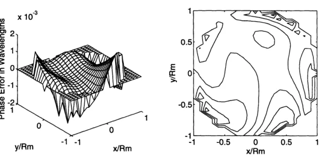
wavefronts at the target, no atmospheric turbulence is added.
CHAPTER 3 R :F; 0m C c a) ca c3 0 l-ca
THERMAL BLOOMING MODEL
-1 -1
Figure 3.7. Typical Wavefront for Light Thermal Blooming.
-1 -0.5 0 0.5 1
-1 -1
Figure 3.8. Typical Wavefront for Heavy Thermal Blooming.
C 3 E 0) 4 1 4 1
THERMAL BLOOMING MODEL
3.7
SUMMARY
In this chapter a model for thermal blooming was presented. At the heart of the model is
data generated by a wave optics code at the Naval Research Laboratory. Using this data, a
number of researchers derived models for thermal blooming in terms of intensity on target
and laser wavefront. This chapter brought together equations from a number of these
models to create a general thermal blooming model that allows for beam focusing. For
inputs, the model takes nineteen atmospheric and target parameters. The primary outputs
of the model are peak intensity on target and the laser wavefront. The wavefront is
expressed in terms of Zernike coefficients corresponding to the focus, astigmatism, coma,
and spherical aberrations. CHAPTER 3
Chapter 4
Atmospheric Turbulence Model
In addition to thermal blooming, turbulence is an important atmospheric effect that must be
considered when evaluating directed energy systems. This chapter presents a dynamic
model of atmospheric turbulence represented in terms of twenty Zernike polynomial
coefficients. In Chapter 6, an extended Kalman filter will be designed to estimate the wind
speed from return wavefront measurements. The Kalman filter does not attempt to estimate
turbulence, but instead uses the turbulence distortion to model measurement noise since it is
likely the most significant contribution.
4.1
TURBULENCE MODEL PARAMETERS
A total of six parameters describe turbulence. The first two parameters can be classified as
atmospheric parameters: wind velocity and the Kolmogorov turbulence structure constant.
The next two parameters describe the laser: aperture radius and wavelength. The final two
parameters are engagement-specific and describe the target's position and velocity. All of
ATMOSPHERIC TURBULENCE MODEL
TABLE 4.1. Atmospheric Turbulence Model Parameters
4.2
ZERNIKE COEFFICIENT MODELING
Turbulence is a random process that causes the index of refraction of the atmosphere and
hence the laser phase profile to be random processes. The phase aberration function, TP,
can be expressed in terms of Zernike polynomials, Pi, and the corresponding Zernike
coefficients, Cj
N
· P(r,0)=
C
i·
Pi(r, 0)
i=1
(4.1)
Each Zernike coefficient is modeled as a random process, the output of a linear filter driven
by unity variance continuous-time white noise. Linear system theory prescribes how to
determine the transfer function of the ith filter, Hi (jo), given the desired power spectral
density function, S.i (o) [18]. The power spectral density function, S.i(w), is factored into
Si(jwo)Si(-jco), where S(jo) is a stable transfer function. The linear filter transfer
function is Si(jo) = KiH(jco).
Parameter Description
Symbol
Nominal Value
Transverse Wind Velocity Uw
2
Turbulence Constant
C
2 xI 10-15mAperture Radius Rm .35m
Wavelength 3.8 X10- 6
Transverse Target Velocity UTX S
Target Distance ZT 5000m
ATMOSPHERIC TURBULENCE MODEL
White Nc
Ci
Figure 4.1. Model for Zernike Turbulence Coefficient.
4.2.1 POWER SPECTRAL DENSITY
It has been shown that the power spectral density of the ith Zernike mode is well
represented by Equation 4.2 [19].
Sii(0)=
4C2k2ZtRmI dd(I{
j
Ih(a
2P)I
0
(mR
2'
V
The various functions and parameters used in Equation 4.2 are defined below.
=1- -Z
ZT II () = 0.033Cn 2 32iv
p
=
-z2
_ (
2n: v o is frequency in rad sz is the along-path distance measurement.
v is the velocity of the beam relative to the air at range z.
(4.2)
(4.3)
(4.4)
(4.5)
(4.6)
CHAPTER 4
ATMOSPHERIC TURBULENCE MODEL
hi is the two-dimensional Fourier transform of the ih Zernike polynomial, given in
Table 4.2.
TABLE 4.2. h-Functions
i h_(a, ) i hi(a,P) _ _)-
2
7 a' ) 2 12 ; J 3<J
13( 8a
+8a
)J4A a2' _P4i -of- (4a3 8a )J,
4
a'
)
14
47
(
a''
S 2
Ia
)
15
Va
a 2 )6
6 -;iE ( )4 16 _ _ _n ____) __ )J 17 1182 (_ 3a + 4a) 7 ____4 a4
17
a
64 J1 3a 4a 4Y 2 3P 4' 8-
4 18n
( 4 9 a*-+4
J4 19 a2 4 - Jh 4fI (F51 203' 161' J1 0
o
20
(
o
+o
a)
Ji is the ith-order Bessel function of the first kind with argument 2na where = _a2 + 2. sin x
J,(x) =
x sin x cos x x2 XJ
(
=
2n-1
Jn> (x) = X JnI (x)- J_2(X)n=0
Jn (0) = O.(4.7)
n>0
CHAPTER 4
ATMOSPHERIC TURBULENCE MODEL
If the target is stationary, or the transverse velocity component is zero, v is simply equal to the transverse wind velocity, Uw. When the target has a non-zero transverse velocity, v
has a component due to the slewing of the beam.
v = UW + UTX(1
- 1)
(4.8)
4.2.2 POWER SPECTRAL DENSITY APPROXIMATION
Researchers at TASC numerically evaluated the power spectral density function given in
Equation 4.2 and used a straight line approximation to more easily represent the data [ 18].
The intersections of the line segments are the corner frequencies of the transfer functions
and correspond to poles and zeros of the transfer functions. Table 4.3 lists the corner
frequencies of the first twenty Zernike modes: f,,a f,Ib fd, and f. These modes all have