Climatology and trends of the middle atmospheric temperature (33–87 km) as seen by Rayleigh lidar over the south of France

HAL Id: insu-03131949

https://hal-insu.archives-ouvertes.fr/insu-03131949

Submitted on 5 Feb 2021

HAL is a multi-disciplinary open access

archive for the deposit and dissemination of

sci-entific research documents, whether they are

pub-lished or not. The documents may come from

teaching and research institutions in France or

abroad, or from public or private research centers.

L’archive ouverte pluridisciplinaire HAL, est

destinée au dépôt et à la diffusion de documents

scientifiques de niveau recherche, publiés ou non,

émanant des établissements d’enseignement et de

recherche français ou étrangers, des laboratoires

publics ou privés.

Climatology and trends of the middle atmospheric

temperature (33–87 km) as seen by Rayleigh lidar over

the south of France

Alain Hauchecorne, Marie-Lise Chanin, Philippe Keckhut

To cite this version:

Alain Hauchecorne, Marie-Lise Chanin, Philippe Keckhut. Climatology and trends of the middle

atmospheric temperature (33–87 km) as seen by Rayleigh lidar over the south of France. Journal of

Geophysical Research: Atmospheres, American Geophysical Union, 1991, 96 (D8), pp.15297-15309.

�10.1029/91JD01213�. �insu-03131949�

JOURNAL OF GEOPHYSICAL RESEARCH, VOL. 96, NO. D8, PAGES 15,297-15,309, AUGUST 20, 1991

CLIMATOLOGY AND TRENDS OF THE MIDDLE ATMOSPHERIC TEMPERATURE (33-87 KM)

AS SEEN BY RAYLEIGH LIDAR OVER THE SOUTH OF FRANCE Alain Hauchecorne, Marie-Lise Chanin, and P. Keckhut Service d'A•ronomie du Centre National de la Recherche Scientifique,

Verri•res le Buisson, Cedex, France

Abstract. The technique of the Rayleigh lidar provides temperature profiles with a good temporal and vertical

resolution in the middle atmosphere. Data obtained by 2

Rayleigh lidars set up at the Observatory of Haute-Provence

(44øN, 6øE) and at Biscarrosse (44øN, IøW) from 1978 to

1989 led to a unique set of data of 1200 night-mean temperature profiles from 37 to 87 km. A climatology of the temperature over the south of France has been established from this data base and new results concerning both the short-

term and long-term variability of the middle atmosphere are

presented in this paper. The observed temperature around

44øN, 0øW is in general colder than the mean temperature

given in the COSPAR International Reference Atmosphere

(1986) near 75 km and warmer above 80 km. A clear semi- annual variation is observed near 65 km with maxima

occurring just after the equinoxes. The study of the short-term variability indicates clearly two frequency domains: long

periods below 65 km with a maximum in December-January

which relate to planetary waves and shorter periods above

65 km induced by the breaking of gravity waves. A correlation with the 11-year solar cycle, negative in the stratosphere and positive in the mesosphere, is found to be well above the 95% confidence level with an amplitude larger in winter than in summer. However, with only 11 years of data it is obviously difficult to conclude that this atmospheric perturbation is induced by the solar forcing. A cooling of the

mesosphere of about -4 K/decade at 60-70 km is found but is

at the limit of the 95% confidence level, whereas we do not

observe any significant trend in the stratosphere.

Introduction

The climatology of the structure of the middle atmosphere

above 30 km has been studied first from in situ rocket

measurements since the 1950s and then by remote sensing

satellite experiments. The rocketsondes provide good vertical

profiles up to 60 km but present some problems of accuracy

beyond 60 km due to the rarefaction of the atmosphere and the very high speed of the sonde. Furthermore, the profile is instantaneous and affected by the short-term gravity waves. The number of soundings is limited by the cost of the launch and the equipment. Falling spheres are used to obtain temperature derived from density measurements up to 90 km [Schmidlin, 1981] but not on a regular basis. Satellite experiments alone are able to give a global coverage of the temperature field but have a relatively low horizontal and

vertical resolution. The mesospheric temperature has been

measured by infrared limb sounders from 1975 to 1982:

Pressure Modulated Radiometer (PMR; Curtis et al. [ 1974]),

Selective Chopper Radiometer [Ellis et al., 1973], Limb Infrared Mesospheric Sounder |Gille et al., 1984] and

Stratosphere and Mesosphere Sounder [Drummond et al.,

Copyright 1991 by the A•ncrican Gc•physical Union.

Paper number 91JD01213.

0148-0227/91/91JD-012135½ }5.()0

1980]. The upper stratosphere is covered continuously by the Stratospheric Sounding Unit instruments (SSU; Miller et al. [ 1980]) on board the NOAA operational satellites, but with a very poor vertical resolution. The climatology of the middle

atmospheric temperature has been obtained by Barnett and

Corney [1985] from PMR data over the 1975-1978 period

and is the base of the new COSPAR International Reference

Atmosphere (CIRA 1986; Barnett and Corney, [1985]). It gives the best available representation of the latitudinal,

longitudinal and seasonal variations of the temperature, at

least up to 65 km. However, the short-term and interannual variability of the atmosphere is not taken into account in the CIRA 1986. This climatology has been completed in the mesosphere by Clancy and Rusch [1989] from global

observations of UV limb radiances from the Solar

Mesosphere Explorer (SME) for the period 1982-1986.

Mesospheric temperature will not be measured from space

until the launch of the Upper Atmosphere Research Satellite at

the end of 1991.

The technique of Rayleigh li 'dar has been shown capable of obtaining temperature profiles with a good vertical resolution from 30 to 90 km and to follow the temporal evolution of this parameter at all time scales from fractions of an hour to years

[Hauchecorne and Chanin, 1980; Chanin and Hauchecorne,

1984]. Two Rayleigh lidars, located in the south of France, are operated about 100 nights per year since 1981 at the

Observatory of Haute-Provence (44øN, 6 ø E) and since 1986

at Biscarrosse (44øN, 1 ø W). The climatology obtained from more than 1000 nightly average profiles will be presented and compared with previous studies. We will emphasize the importance of temperature variance associated with different phenomena, planetary wave propagation, breaking of gravity waves, quasi-biennial oscillation (QBO) and the 11-year solar cycle.

Lidar description

Data used in this study have been obtained with the Rayleigh lidar technique, which is based on the backscattering of a pulsed laser beam by atmospheric molecules. The temporal analysis of the echo provides the vertical profile of atmospheric density in relative value. The temperature profile is deduced from the density profile using classical hypothesis, hydrostatic equilibrium and perfect gas law, and is obtained in absolute value. The method is described in detail in previous publications [Hauchecorne and Chanin, 1980; Chanin and Hauchecorne, 1984] and only indications relevant to this study will be given here.

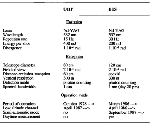
The experimental data set has been obtained from October

1978 to December 1989 with two lidar stations based in the

south of France: Observatory of Haute-Provence (OHP, 44øN, 6øE) and Biscarrosse (BIS, 44øN, IøW). The main characteristics of the two lidars are presented in Table 1.

The quality of the data at OHP has been improved in December 1983 by using a more powerful data acquisition system. The BIS lidar may be operated during daytime by using a smaller field of view (0.1 mrad) and a Fabry-Perot interferometer to reduce the background light. However, temperature profiles are limited to 60 km in this mode and will not be used in the climatological study.

15,298 Hauchecorne et al.: Rayleigh Lidar Temperature Climatology

Table 1. Lidar characteristics

OHP BIS

Emission

Laser Nd-YAG Nd-YAG

Wavelength 532 nm 532 nm

Repetition rate 15 Hz 30 Hz

Energy per shot 400 mJ 200 mJ

Divergence 1.10-4 rad 1.10-4 rad

Reception

Telescope diameter 80 cm 120 cm

Field of view 2.10 -4 rad 2.10 -4 rad

Distance emission-reception 60 cm coaxial

Vertical resolution 300 m 300 m

Detection mode photon counting photon counting

Spectral bandwidth 1 mn 1 nm (day 20 pm)

Period of operation

Low altitude channel Semi-automatic mode Daytime measurement Operation mode October 1978 ---> March 1986 ---> April 1987 ---> April 1986 ---> no September 1988---> no yes

Discussion of the method The Role of Mie Scattering

The Rayleigh lidar method assumes that the scattering light is only due to Rayleigh scattering by molecules and that the Mie scattering due to aerosols is negligible. Due to the presence of the stratospheric aerosols layer around 20 km, it is

not possible to use measurements below 30 km. Multi-

wavelength measurements have shown that outside the periods following major volcanic eruptions the Mie scattering

contribution may be neglected above 30 km. However, after

the E1 Chichon eruption in May 1982 aerosols have been detected as high as 38 km lLefr•re et al., 1981] and data

contaminated by aerosols have been suppressed in 1982 and

1983 for the data base used in this paper.

Hydrostatic and Constant Mixing Ratio Hypothesis

The determination of the temperature from the density

profile is based on the assumption that the atmosphere is in hydrostatic equilibrium. This is not true locally in strong

turbulent layers; however, taking into account the time and

spatial integration of the lidar measurement, such an hypothesis is verified with a good level of accuracy. It is also assumed that the major gases of the atmosphere are in constant mixing ratio, which is true up to the homopause near 100 km.

Above this level the mean molecular weight of the atmosphere

slowly decreases with height.

Optic and Electronic Effects

The determination of the temperature assumes that the

measured scattering is proportional to the atmospheric density divided by the square of the distance, with a constant of proportionality independent of the altitude. This constant may be affected by two types of problems:

Focalization and parallax effects. The scattered light is

collected at the focus of the reception telescope but this focus depends on the altitude of the scattered light. In addition, if the emission and the reception telescopes are not coaxial, an effect of parallax depending on the altitude is observed. In order to minimize these effects it is necessary to reduce the divergence

of the laser beam, to minimize the distance between the

emission and the reception, to have a telescope field of view large enough to include all these effects and to rely on a very good procedure to check the parallelism between the two telescope axis.

Dynamic of the signal. Two of the problems of the Rayleigh lidar are the large dynamic of the signal which varies

by a factor

of 105 from 30 to 90 km and the very high

light by the lower atmosphere. These difficulties are resolved by using a mechanical or an electronic shutter to protect the detector from the lower atmosphere diffusion and by adding a second detector, which receives a few percents of the signal, for the lower part of the profile.

Accuracy

Errors affecting these measurements may be divided into

two parts:

1. The statistical error due to the photon counting is easy to evaluate. This error is reduced when the temporal and spatial resolution are degraded. For long-term trends and planetary wave studies, average nighttime profiles are used, integrated during 3 to 4 hours and with a 3 km vertical resolution. In this case, the typical values of the statistical error from 30 to 70 km < 0.3 % in density <IK in temperature

at 80 km 1% in density 3 K in temperature

at 90 km 3 % in density 10 K in temperature

2. Due to the optic and electronic problems mentioned above, a source of systematic errors may appear in the measurements and is very difficult to evaluate. In order to

Hauchecorne et al.: Rayleigh Lidar Temperature Climatology 15,299

simultaneously at the two lidar sites during 65 nights have been compared. The two lidars are at the same latitude and 550 km apart; it is to be expected that the mean temperature profile will not be very different within this distance. At all altitudes

between 30 and 80 km this difference has been found to be less than 2 K and this value is therefore an estimate of a

possible systematic error. Comparison with radiosondes data at 30 km also indicate the same order of accuracy.

Data base

The data base consists of one mean temperature profile per night of measurement for each lidar site from October 1978 at

OHP and March 1986 at B IS until the end of 1989 at both

sites. The number of nights of measurements per month for

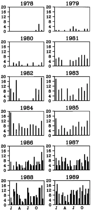
each site is presented in Figure 1. During the recent years a mean value of eight nights per month is obtained at each site with a maximum as high as 19 nights per month in January 1984 at OHP. For the whole period the number of nights is

872 at OHP and 328 at BIS.

The two stations are located at the same latitude (44 ø N)

from 550 km apart which is a short distance compared to the

wavelengths of planetary waves (a few thousands of kilo-

meters). It is then reasonable to consider that the climatology

of the temperature is the same at the two sites and to use

together all the data obtained at BIS and at OHP in a single set of data representative of the south of France. The number of

profiles per month obtained this way allows a finer temporal

description of the temperature variations.

Experimental Results

Mean Temperature

Data at OHP are of better quality and of extended height

range since December 1983; the mean climatology of the

temperature has been established by using data only from 1984 to 1989. Data obtained before 1984 will be used only to study long-term variations of the temperature.

The seasonal evolution of the temperature is obtained as follows: for each year from 1984 to 1989, data are interpolated to obtain one value per day and per kilometer. Data are

smoothed with a 30-days FWHM Hanning filter. Finally for

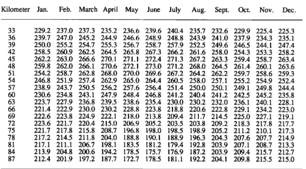
each day of the year the mean value is computed for the 6-year period and the results are presented in Plate 1 and tabulated in Table 2 by steps of 3 km in altitude and for the fifteenth of

each month.

In spring and summer the evolution of the temperature is classical with the maximum at the stratopause and the

minimum at the mesopause occurring in May/June, slightly

before the summer solstice. In the upper stratosphere the

minimum occurs at the beginning of November, one month

and a half before the winter solstice, and is associated with a

maximum in the 60- to 70-km range. A relative maximum is

observed at the end of February in the middle stratosphere.

The winter evolution may be explained by the frequent

occurrence of upper stratospheric warmings in January and

February, which increases the mean temperature during that

period. A semiannual variation is seen clearly around 65 km with maxima in March/April and October/November.

The lidar climatology has been compared to the CIRA 1986 in which the contribution of planetary waves 1 and 2 has been included (Plate 2 and Table 3). Below 65 km the agreement between the lidar climatology and the CIRA 1986 is in general

very satisfactory with differences smaller than 5 K, if we

except a positive deviation observed in the middle stratosphere

in February, corresponding to the frequent occurrence of

stratospheric warmings during this month. In the altitude range

of 65-80 km, lidar temperatures are in general colder than

CIRA 1986 with a deviation larger than 10 K at 75 km in May

and in November. On the contrary, positive deviations from

CIRA 1986 are observed above 83 km with values as high as

1978

1979

4

I 4

,,

, ill,

ii

1980

1981

o I,I m I i 4

1982

1983

0

m

m

0

'

ß

1984

1985

16]

16

1986

1987

1988

Fig. 1. Monthly

number

of data

nights

at OHP (solid)

and

BIS

(shaded).

18 K at 87 km in September. Temperature profiles obtained at

45øN from SME limb scattering data I Clancy and Rusch,

1989], which are in good agreement with our lidar data in

absolute value (see also Aikin et al. [1991] for the SME-lidar comparison), also show positive deviations compared to CIRA 1986 from 65 to 80 km and negative deviations above 80 km.

The mean temperature and its annual and semiannual

components have been extracted by use of a least squares fit on data from 1984 to 1989 as explained in Appendix 1, but

87 81 75 30 69 I-- 57 51- 45- 39-- F M A M J J A S O N D SUP 270 iiii,i.i,i•i:,•.i..!•; 260 - 270 •'" .... ' 250 260 240 - 250 .,& .... • 230-240 ,. ... '; 220 - 230 210 - 220 200- 210 190 - 200 .. ' 180- 190 INF 180 DATA FROM 1 1 1984 TO 31 12 1989

Plate 1. Time-height section o1' the temperature over the south of France obtained with data from 1984 to 1989. A 30-day Hanning filter has been applied to the data.

75 "

•' 63

• 57

i?'.,•::_..:.,.,.'?::'::"h":"':•:':

...

: ,,,.-' ...

Plate 2. As in Plate 1 but for the deviation from CIRA 1986.

SUP 14,0 11,0- 14,0 8,0- 11,0 5,0- 8,O 2,0 - 5,0 -1,0 - 2,0 -4,0 - -1,0 -7,0 - -4.0 -10,0 - -7,0 -13,0 - -10,0 INF -13,0

81 75- 69-

63-

j

F

M

A

M

J

J

A

S

O

N

D

....,.._-J

63-

Plate 3. Standard deviation •)t' the tCml)crature (data from 1984 to 1989) corresponding to I)crtt, rbations with 2-to 30-day periods (see text). A 30-day i i;tnning filter has been applied to the data.

III IIII!1 !1 !111 I!/ I•llllll Ill .t II I II II 11 I IOHP

il IllIll I IllBIll Ill IIII II Illllll111181S

180

80 81 82 83 84 85 86 87 88 89

Plate 4. Temperature deviati()n from the climatological average presented in Plate l. Dates of

measurement at OHP and BIS are shown in the upper part of the figure. A 180-day Hanning

filter has been applied to the data.

SUP 9.0 7.0- 9.0 5.0- 7,0 3.0- 5.0 1.0- 3.0 -1.0- 1.0 -3.0 - -1.o -5.0 - -3.0 -7.0 - -5.0 -9.O - -7.0 INF -9 0

15,302 Hauchecorne et al.: Rayleigh Lidar Temperature Climatology

Table 2. Mean Temperature Profile Tabulated for the Fifteenth of Each Month (Data From 1984 to 1989)

Kilometer Jan. Feb. March April May June July Aug. Sept. Oct. Nov. Dec.

33 36 39 42 45 48 51 54 57 60 63 66 69 72 75 78 81 84 87 229.2 237.0 237.3 235.2 236.6 239.6 240.4 235.7 232.6 229.9 225.4 225.3 239.7 247.0 245.2 244.9 246.6 248.9 248.8 243.9 241.0 237.9 234.3 235.1 250.0 255.2 254.7 255.3 256.7 258.7 257.9 252.5 249.6 246.5 244.1 247.4 258.5 260.9 262.5 264.5 265.8 267.3 266.2 261.6 258.0 254.3 253.3 258.2 262.2 263.0 266.6 270.1 271.1 272.4 271.3 267.2 263.3 259.4 258.7 263.4 259.8 262.0 266.1 270.6 272.1 273.0 271.2 268.0 264.5 261.4 260.1 263.6 254.2 258.7 262.8 268.0 270.0 269.6 267.2 264.2 262.2 259.7 258.6 259.3 246.8 251.9 257.4 262.9 265.0 264.4 260.5 258.0 257.1 255.2 254.9 252.4 238.9 243.7 250.5 256.2 257.6 256.4 251.4 250.0 250.1 249.1 249.8 244.4 230.6 234.8 243.1 247.9 248.4 246.8 241.2 240.4 241.2 242.5 245.2 235.8 223.7 227.9 236.8 239.5 238.6 235.4 230.0 230.2 232.0 236.1 240.1 228.1 221.4 222.9 230.0 230.2 228.8 223.8 218.8 220.6 222.8 229.1 234.2 223.0 222.6 223.8 224.9 222.1 218.0 213.8 209.4 211.7 214.5 225.0 227.1 219.1 223.6 221.7 220.4 215.0 206.9 205.2 203.5 203.8 209.2 218.3 217.8 217.7 221.7 217.8 215.8 208.7 196.8 198.0 198.5 198.9 205.2 211.2 210.1 217.3 217.2 214.5 211.8 204.0 188.8 190.1 188.9 196.3 204.3 207.6 207.7 214.9 217.1 211.1 206.7 198.1 183.5 181.2 179.4 192.8 203.9 207.1 208.7 213.3 213.9 204.8 200.6 194.2 178.5 175.7 176.9 187.2 203.9 209.4 215.7 212.7 212.4 201.9 197.2 187.7 172.7 178.5 181.1 192.2 204.1 209.8 215.5 215.0

Table 3. Mean Temperature Deviation from the CIRA 1986 Tabulated

for the Fifteenth of Each Month (data from 1984 to 1989)

Kilometer Jan. Feb. March April May June July Aug. Sept. Oct. Nov. Dec.

33 36 39 42 45 48 51 54 57 60 63 66 69 72 75 78 81 84 87 -5.9 5.8 3.5 -3.4 -3.9 -2.4 -0.9 -3.1 -2.4 0.6 2.5 -3.7 -3.5 6.7 0.7 -4.1 -3.9 -1.8 -0.1 -2.1 -1.3 0.9 2.7 -3.0 -1.2 5.8 0.3 -3.2 -3.2 -0.6 1.3 -1.1 -0.6 0.9 2.8 -0.1 0.8 4.1 0.2 -1.5 -1.9 0.4 2.6 1.1 0.5 0.5 2.5 2.9 0.7 1.8 -0.2 -0.3 - 1.3 0.7 3.2 2.2 0.5 -0.9 1.0 3.1 -1. 0.4 -1.1 -0.2 -0.7 0.4 2.1 2.0 -0.3 -1.8 -0.6 2.2 -2.4 1.4 -0.4 0.9 0.4 -0.3 0.6 1.0 0.1 -1.3 -0.6 1.2 - 1.6 2.0 1.6 2.8 1.9 {).2 -0.4 0.9 1.6 -0.1 0.6 0.7 -0.6 1.9 3.3 4.8 3.3 0.4 -2.0 0.3 2.9 1.2 1.9 0.1 - 1.9 -0.5 3.3 4.5 2.9 0.2 -3.4 - 1.5 1.9 1.8 3.8 -2.0 -4.2 -3.3 2.3 2.4 1.1 -1.4 -4.8 -3.3 0.2 2.4 4.3 -4.7 -3.6 -5.4 -0.5 -1.4 -1.1 -3.2 -6.0 -4.8 -2.2 1.7 3.2 -6.0 -0.4 -2.0 -2.2 -4.1 -4.1 -3.6 -6.4 -6.4 -4.7 2.7 0.1 -6.7 1.6 -2.4 -3.6 -5.9 -7.6 -3.2 -3.9 -7.6 -5.2 -0.1 -6.0 -6.0 0.5 -4.4 -4.5 -6.5 -10.1 -2.0 -0.9 -5.9 -5.1 -4.2 -11.1 -4.5 -2.7 -4.9 -3.9 -4.5 -9.8 -1.4 -2.3 -1.8 -2.2 -5.2 -11.4 -5.1 -0.9 -4.8 -3.6 -3.1 -6.8 -1.9 -3.7 1.5 2.0 -2.4 -7.8 -4.6 -0.5 -5.6 -2.6 1.3 -3.3 0.6 1.3 3.5 9.2 5.8 4.6 - 1.5 4.5 -0.5 3.2 4.1 - 1.2 9.8 11.5 16.4 18.6 14.8 12.8 7.8

without taking into account the long-term trend and the response to solar activity that will be discussed later. In the mean temperature profile (Figure 2) the stratopause is located at 47 km with a temperature of 267 K and the mesopause at 86 km with 196 K. The temperature gradient is maximum

between 35 and 40 km with +3.2 K/kin and minimum between 55 and 65 km with-2.7 K/kin.

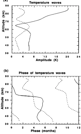
The annual wave (Figure 3) has a nearly constant

amplitude of about 6 K from 33 to 57 km, a node at 65 km and

an increasing amplitude up to the mesopause (21 K at 86 km). The maximum is observed in May-June, in phase with the solar heating below the node at 65 km and is in anti-phase with the solar heating above 65 km with a maximum occurring between November and January.

The semiannual wave (Figure 3) presents a maximum of

amplitude of 6 K at 61-66 kin, around the altitude of the node of the annual wave, which explains the quasi-purely semi- annual variation of the temperature at 65 km already

mentioned.

Short-Term Variability Temperature

Previous climatologies of the temperature in the middle

atmosphere did not take into account the notion of variance,

which is very important when one has to use this climatology

to forecast expected temperatures and to compare it with

observed profiles. To study this variance we define a short-

Hauchecorne et al.' Rayleigh Lidar Temperature Climatology 15,303

9O

.--•60

5O

4O

Mean temperature profile

-

3O 1

190 200 210 220 230 240 250 260 270

Temperature (K)

Fig. 2. Mean temperature profile over the south of France

(data from 1984 to 1989). (a) 9O E80 •70 'o •60 5O 4O 3O Temperature waves ' I ' ' ' I ' ' ' I , I , , , I , , , I , ß 8 12 16 Amplitude (K) 24

temperature due to perturbations with periods ranging from 2 to 30 days. It is defined as a function of the temperature T(t) as

In this formula the overbar denotes a Hanning filtering over 30 days. This variability is mainly due to the propagation of planetary waves. Data are integrated for 3 to 13 hours each night and then the contribution of the gravity waves tends to be eliminated, although long-period inertio-gravity waves may still contribute to the variability. Data are usually obtained during the first half of the night and then the contribution of tides, which become important above 65 km [Gille et a1.,1991], may be neglected in this study.

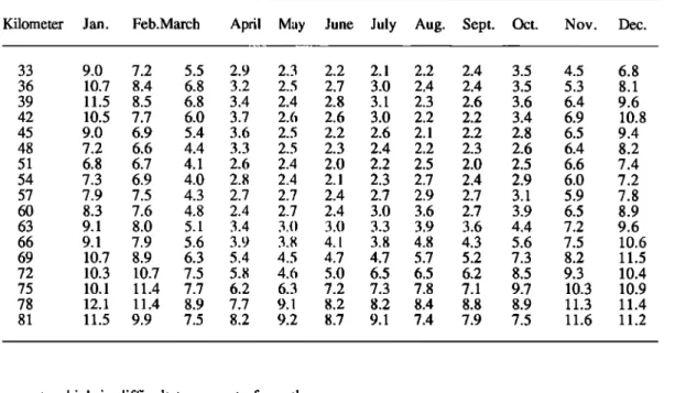
In the stratosphere (Plate 3 and Table 4) the variability is

maximum in December/January with values up to 10 K at 40

km and is lower than 3K from April to October. This variability is clearly related to the propagation of planetary

waves and the occurrence ot' upper stratospheric warming

during the period of strong westerly winds in the lower

stratosphere in winter and the blocking of these waves when

the wind blows from the east in spring and summer

[Hauchecorne and Chanin, 1983].

In the mesosphere a minimum of variability is observed in

winter just above the stratopause at 50-55 km, corresponding

to a quiet layer between the upper stratospheric warmings and the associated mesospheric coolings, which leads to an important variability up to the higher levels. The minimum of variability from April to October still exists in the lower

mesosphere up to 65 K, but above this level the variability

remains large during the whole year (higher than 7 K at 78

km). The summer variability may be partly explained by the

propagation of short-period planetary waves (for instance 2- day and 5-day waves) which are able to propagate through the easterly winds due to their high westward phase speed [Salby,

1984]. But another important phenomenon that more likely

explains this variability is the occurrence of mesospheric

temperature inversions due to the breaking of gravity waves

above 70 km. Hauchecorne et al. 119871 have shown that

these inversions even though more frequent in winter also appear in summer and may persist for several days. They should then contribute to the day to day variability all year

round.

Long. Term Variability and Trend

As the lidar data base covers now a full 11-year solar

cycle, the data have been analyzed in order to separate an

(b)

Phase of temperature waves

,,2 / 80 ' ,, - • 70 '', -- •60 • • - •50 ,. - 40 '-, - 0 2 4 6 8 10 12 Phase (months)

Fig. 3. (a) Amplitude of the annual (solid curve) and semi-

annual (dashed curve) temperature waves over the south of

France (data from 1984 to 19•9). (b) Phase of the annual and

semiannual temperature wavc•. A value of 0 •o• the phase co•csponds to a maximum al Ihc !)c•inning of Janu•y and ]2

at •c end of December.

eventual long-term trend of anthropogenic origin from the

variation due to the 11-year cycle.

Data have been filtered with a 180-day Hanning filter to eliminate short-term variations due to planetary waves. The results between May 1979 and December 1989 are presented in Plate 4. The temperature presents quasi-periodic variations with 2 to 3 years periods probably associated with the QBO. A longer period evolution is also visible with cold temperatures

in the stratosphere during the two solar maxima in 1979-1982

and in 1988-1989 and warm temperatures during the solar

minimum in 1985-1987. in the mesosphere the temperature

follows the opposite evolution with warm temperatures during the solar maxima and cold temperatures during the solar

minimum.

In order to separate the response to the solar forcing from a long-term linear trend, a least squares fit has been made on

data obtained from January 1979 to December 1989 using the

method explained in Appendix 1 with an estimation of the confidence intervals as explained by Frederick 119841. This fit has been first applied to the whole set of data with the seven parameters of the fit and second to the data obtained during the six "summer" months from April to September and the six

15,304 Hauchecorne et al.- Rayleigh Lidar Temperature Climatology

Table 4. Mean Standard Deviation of the Temperature Tabulated

for the Fifteenth of Each Month (Data from 1984 to 1989)

Kilometer Jan. Feb. March April May June July Aug. Sept. Oct. Nov. Dec.

33 9.0 7.2 5.5 2.9 2.3 2.2 2.1 2.2 2.4 3.5 4.5 6.8 36 10.7 8.4 6.8 3.2 2.5 2.7 3.0 2.4 2.4 3.5 5.3 8.1 39 11.5 8.5 6.8 3.4 2.4 2.8 3.1 2.3 2.6 3.6 6.4 9.6 42 10.5 7.7 6.0 3.7 2.6 2.6 3.0 2.2 2.2 3.4 6.9 10.8 45 9.0 6.9 5.4 3.6 2.5 2.2 2.6 2.1 2.2 2.8 6.5 9.4 48 7.2 6.6 4.4 3.3 2.5 2.3 2.4 2.2 2.3 2.6 6.4 8.2 51 6.8 6.7 4.1 2.6 2.4 2.0 2.2 2.5 2.0 2.5 6.6 7.4 54 7.3 6.9 4.0 2.8 2.4 2.1 2.3 2.7 2.4 2.9 6.0 7.2 57 7.9 7.5 4.3 2.7 2.7 2.4 2.7 2.9 2.7 3.1 5.9 7.8 60 8.3 7.6 4.8 2.4 2.7 2.4 3.0 3.6 2.7 3.9 6.5 8.9 63 9.1 8.0 5.1 3.4 3.{} 3.0 3.3 3.9 3.6 4.4 7.2 9.6 66 9.1 7.9 5.6 3.9 3.8 4.1 3.8 4.8 4.3 5.6 7.5 10.6 69 10.7 8.9 6.3 5.4 4.5 4.7 4.7 5.7 5.2 7.3 8.2 11.5 72 10.3 10.7 7.5 5.8 4.6 5.0 6.5 6.5 6.2 8.5 9.3 10.4 75 10.1 11.4 7.7 6.2 6.3 7.2 7.3 7.8 7.1 9.7 10.3 10.9 78 12.1 11.4 8.9 7.7 9. I 8.2 8.2 8.4 8.8 8.9 11.3 11.4 81 11.5 9.9 7.5 8.2 9.2 8.7 9.1 7.4 7.9 7.5 11.6 11.2

annual component, which is difficult to separate from the annual component with only six months of data per year.

The square root of the variance, obtained from the random term of the fit (see Appendix 1) (Figure 4a), is different from the short-term variability presented in Plate 3. It contains both the variability due to perturbations of periods longer than 7 days but shorter than 6 months and the interannual variability not taken into account by the fit. However, the results are quite similar to those presented in Plate 3, with values higher in winter than in summer and a relative minimum of variability near 50 km and large values all year round in the upper

mesosphere.

The correlation between two successive 7-day profiles

(Figure 4b) is nearly constant at 0.4-0.45 up to 65 km and

decreases abruptly beyond 65 km to reach values lower than

0.2 at 75 km. These values correspond to a time constant t of

the temperature autocorrelation (see Appendix 1) of about 9

days below 65 km decreasing to 4 days at 75 km. This result

indicates that the variability is controlled by the planetary wave activity up to 65 km, with typical periods ranging from 1 week to 1 month, and by the breaking of gravity waves above 65 km which induces temperature perturbations as mesospheric inversions persisting a few days Ittauchecorne et al., 1987;

Hauchecome and Maillard, 19901.

When we consider the whole set ot' data (Figure 5a), the response to solar flux is well above the 95% confidence level

and near the 99.99% level (about 4 o) at maxima, with a

negative response in the stratosphere and a positive response in the mesosphere. The maxima are obtained around 38 and 67

km with-3.8 K and +4.4 K/100 units of 10.7 cm flux (100

FU), respectively and a node is observed around 50 km. If this response is due to a radiative forcing of the middle

atmosphere, we may expect a larger response in summer than

in winter. The opposite is observed (Figure 5b for summer and Figure 5c for winter). The response has the same shape in summer as in winter but with a smaller amplitude. In summer

the +2.7 K/100 FU response in the mesosphere is still

significant at 95 % due to a small confidence interval related to the low short-term variability of the atmosphere, but the -1.1 K/100 FU response in the stratosphere is well below the 95% level. In winter the-5.7 K/100 FU stratospheric and +5.4 K/100 FU mesospheric responses are significant at 95%, in spite of the large short-term variability. This difference in the

(a) •0 8o •3 60 • 50 4O 3O

Variability of the temperature

summer ,, , • o .. _ t . . i ß ß _ • _ , _ , 0 2 4 6 8 10 Standard deviation (K)

(b)

Temperature

autocorrelation

'7o

Fig. 4. (a) Variability of the tc•nperature corresponding to the

random term of the least squares fit (see Appendix 1). (b)

Correlation between two successive 7-day mean temperature

Hauchecorne et al.' Rayleigh Lidar Temperature Climatology 15,305 (a) 8O .•_60 5O 4O 3O (b) 80 •70 •60 5O 4O 3O

Correlation with 10.7 cm flux, all data

- ß

_

"

confidence_

_

Correlation with 10.7 cm flux, summer

, _ .. - t , i _ ', , _ ß _ ' 95% confidence I -10 -8 -6 -4 -2 0 2 4 6 8 10 K / 100 flux units at 10.7 cm (c) 80 E •70 ,•60 5O 4O

Correlation with 10.7 cm flux, winter

95% confidence

30 , I , I , I , I ,

-10 -8 -6 -4 -2 0 2 4 6 8 10 K / 100 flux units at 10.7 cm

Fig. 5. Response to the 10.7-cm solar flux obtained with the least squares fit for (a) all the data, (b) summer months and

(c) winter months (data from 1979 to 1989).

seasonal behavior indicates thai we need to consider the role of

the dynamics and in particular of the propagation of planetary waves in the possible link between the solar activity and the

temperature of the middle atmosphere. The present study

shows that a periodicity around 11 years exists in the lidar data. However, our data set covers only one solar cycle and one should be careful before concluding that this periodicity is due to the 11-year solar cycle and is not a natural fluctuation of the Earth atmosphere.

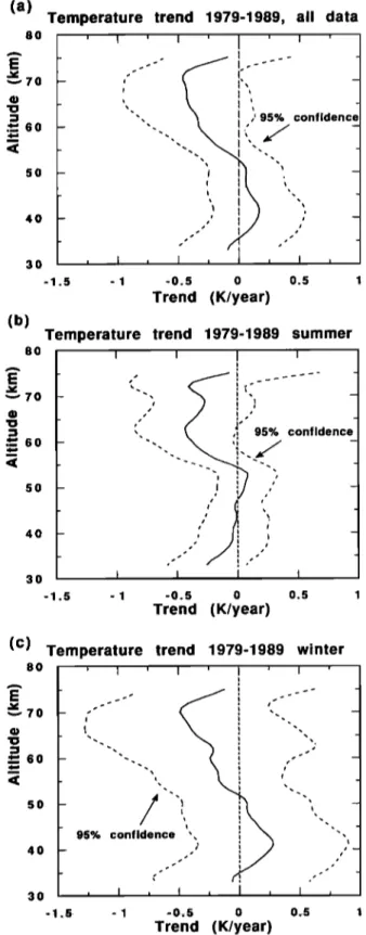
The linear trend observed on the whole set of data (Figure 6a) is positive but well below the 95% level in the stratosphere

and negative in the mesosphere and at the limit of the 95%

(a) 8O .•_60 5O 4O 3O (b) 8O •60 5O 4O 3O

Temperature trend 1979-1989, all data

-

,.

, I I I I I • I

-1.5 - I -0.5 0 0.5 1

Trend (K/year)

Temperature trend 1979-1989 summer

, , ;. ,I 95% confidence // i - .ß/ ./" I I I I -1.5 - I -0.5 0 0.5 Trend (K/year) (c) 8O •60 5O 4O 3O

Temperature trend 1979-1989 winter

,,

- 95% confidence

',.

i "•

"

-1,5 - I -0.5 0 0.5

Trend (K/year)

15,306 Hauchecorne et al.: Rayleigh Lidar Temperature Climatology

level at 70 km with -4.6 K/decade. Due to the confidence

interval being smaller in summer than in winter, we may expect an easier detection of the trend in the former case. This is true in the mesosphere where the negative trend is in the order of-4 K/decade between 60 and 70 km during both

seasons (Figure 6b for summer and Figure 6c for winter) but

above the 95% level in summer and not significant at all in

winter. In the stratosphere no significant trend is observed in

both seasons.

For the determination ol' a trend the confidence interval

decreases rapidly when the number of observations n increases

(it is proportional

to n-3/2 following

Frederick

[1984]).

Furthermore the maximum of the present solar cycle occurred

at the beginning of 1990. Data obtained during the decrease of the solar cycle will be crucial to confirm or to contradict the present results. For instance from our results in the

mesosphere we expect a strong cooling near 65 km due to the

positive response to the solar flux and the negative linear

trend.

Discussion

In order to compare these results on long-term variability

with previous observations, one has to be aware that trends

have sometimes been deduced from data sets of very short

duration (about half of a solar cycle). Since model predictions generally underestimate the amplitude of the solar influence, the incorrect estimate of the part due to the solar change led to large uncertainty on the determination of the trend itself. Influence of the 1 I-Year Solar Cycle

The middle atmosphere between 30 and 70 km is expected

to respond to changes in UV solar flux, in particular, the 11- year cycle period. The photo-chemical models IGarcia et al., 1984; Brasseur, 1989] predict a maximum effect of the 1 l- year solar forcing of +1 K at 50 km and a negligible effect out of the 30-to 70-km height range. This response is quite smaller

than what was shown by observations and the disagreement

stays unexplained.

Using radiosonde data, l,abitzke and van Loon 119881 have shown that the temperature in the winter stratosphere at

30 hPa is correlated with the solar flux and that this correlation

is improved when the data are separated itccording to the phase

of the QBO. These results have been extended to the upper

stratosphere and the mesosphere by Labitzke and Chanin

[1988] using rocketsonde and lidar data and by Chanin et al.

[1989] in the lower thermosphere. Keckhut and Chanin 11989]

and Chanin [ 1989] have shown from lidar data at OHP from 1979 to 1988 that the observed effect for all seasons and

independently of the sign of the QBO is -3 K/100 FU at 40 km

and +7 K/100 FU at 65 km and that the correlation tends to

become negative above 80 kin. This last point is confirmed by the recent data of Neumann 1199()1 who found a negative

response of-4K/100 FU at 86 km using OH temperature data

obtained at Wuppertal (50øN, 7øE). A strong positive correlation between mesospheric temperature and solar flux is also observed at other sites of both high and low latitudes from

rocketsondes data [Mohanakumar, 19891.

These results are also consistent with the cooling of the mesosphere during the descent of solar cycle n ø 21 as observed by SSU (Channel 47X) between 1979 and 1986 I WMO,

1989] and SME temperature between 1982 and 1986 IClancy

and Rusch, 1989] which indicate changes of -1 K/year at 0.5 hPa (about 55 kin) and-1.5 K/year between 60 and 70 km respectively (the analysis ol' the lidar data during the period 1982-1986 indicates a negative trend of-1 K, -1.2 K, -1.7 K and- 1.4 K/year at 55, 60, 65 and 70 kin, respectively).

The whole set of observations gives the following picture: a positive response of 1 K below 30 kin, a negative one of-3 to -4 K at 40 km turning to positive around 50 km with a

maximum

of +5 to +7 K between

60 and 70 km and again

changing to negative at the mesopause height. Those results

are confirmed by the results presented earlier but are not yet

understood.

Anthropogenic trends'

Global climatic models predict a warming of the troposphere due to the industrial emissions of carbon dioxide and other greenhouse gases such as CH4, N20, CFCs [Hansen et al., 1983]. This warming should be associated

with a cooling in the middle at•nosphere, due to the IR

emissions of these gases into space. Additional processes are likely to affect the stratosphere, a•nong which are the ozone change and the increase in aer•sol concentration. As a consequence of the induced n•diativc perturbations, dynamical

processes and wave propagation could appear.

Therefore modelling of these complex interactions are not

yet complete. The one-dimensional coupled photochemical

model of Briihl and Crutzen 119881 for the scenario 1, the

closest to the period 1960-1985, leads to a cooling of-1.5

K/decade for the recent pltst at 45-50 km. The two-

dimensional model of Brasscur and Hitchman [1988l predicts

a cooling of 20 K at 50 km for a doubling of CO2 and an

increase of Clx from 2.0 to 6.6 parts per billion in volume and its extention to the mesosphere by Robie and Dickinson ! 1989]

predicts a 10 K cooling in the upper mesosphere for a

doubling of CO2 and CH4. Using tile 3-D Goddard Institute

for Space Studies model which only includes the effect of

greenhouse gases but takes into account changes in dynamics,

Rind et al. [1990] obtained a lowest value of 10 K at 55 km.

Within a factor of 2 the agreement between those recent models is quite satisfactory: they all indicate a maximum effect

around 50 km and a rate of cooling between 1 and 2 K/decade

for the present period. It is to I)e noted Ihat these results are not very different from the results of era'lief predictions by a dozen of 1-D radiative photochc•ical models which had been compared [WMO, 19891 and which predicted a cooling of- 1.5 K to- 1.7 K/decade in the 40- to 50-kin layer.

The experimental evidence of trends suffers from the shortness of the data set. The longest series is clearly the one

provided by radiosondes. Using the Berlin data set, Labitzke

et al. [1986] found a negative trend in the temperature at 30

hPa from 1966 to 1980 of-0.24 K/decade over the whole

northern hemisphere and -0.48 K/decade at 40øN. However in a recent publication van Loon and Labitzke 119901 raised the question of the significance of these results considering the

high variability and the large amplitude of the 10-12 year

oscillation. They concluded that more cycles of data were

needed to detect an unambiguous trend. Above 30 kin, data are of shorter extent if we except the rocket data for which the change of the calibration pnx:cdure in the early 1970s may be a source of uncertainty. However, usi•g data obtained after the change, Angell [19871 found a li•ear trend for the period 1973-1985 of -0.4 K, -1.2 K and-2 K/decade in the 26-35,

36-45 and 46-55 km layers, respectively.

In the mesosphere, temi)eraturc da•a are fewer and cover one solar cycle at most. Recently, tile SSU 47X data were reanalyzed and led to a te•npcraturc decline ot' 3.5 _+ 0.5 K in the 1980-1990 decade at 0.5 hPa IAikin et al., 1991 I. Indirect evidence of a cooling has been •bscrvcd by Taubenheim et al. [1990] from the reflection height ot' n•dio waves that showed a

decrease of 10% of the air pressure at 80 km from 1962 to

1987 corresponding to an average 4 K cooling of the whole

mesosphere (1.6 K/decade). Another indirect evidence can be provided by the occurrence of noctilucent clouds as suggested

by Thomas et al. [1989]; Gadsen 11990] using a 25-year

analysis of visual observations reports a 250% increase in nocfilucent clouds occurrence which could be resulting from a cooling of 6.4 K over the same period of 2 K/decade at 90 km.

Hauchecorne

et al.' Rayleigh

Lidar

Temperature

Climatology

is in good agreement with SSU channel 47X and compatible

with the indirect evidence in •hc 80-90 km height range but 2 to 4 times larger than expected by Ire models.

On the contrary, the expected c{xfling of the stratosphere is

not observed and even the !idar data seem to indicate a

tendency toward a warming. This fact may be due to a change

in the planetary wave activity during the period of analysis that tends to cancel the trend in the stratosphere and to amplify it in the mesosphere at the lidar site longitude. We have to keep in mind that our measuremenls are i•cal and that •nodels usually give zonal mean predicti•s. Tl•cy may differ from local

results as climatic conditions may generate cooling in some

places and warming in others.

Conclusion

Data obtained by two Rayleigh lidars set up at OHP and

BIS from 1978 to 1989 allowed us to obtain a unique set of data of 1200 nightly mean temperature profiles from 30 to 90

km. A climatology of the temperature in the middle atmosphere

over the south of France has been established from this data

base. The main results of this study are summarized below: 1. The observed temperature is in general colder than in the

CIRA 1986 near 75 km and warmer above 80 km.

2. A clear semiannual variation is observed near 65 km

with maxima occurring just after tile equinoxes.

3. Below 65 km the short-term variability (periods ranging

from 2 to 30 days) is maximunl in December-January and very

low from April to September. It is •nainly due to the upward

propagation of planetary waves with periods longer than 1

week.

4. Above 65 km a large short-fetal variability is observed

during the whole year, associated with the breaking of gravity

waves that induce temperature perturbations as mesospheric

inversions persisting a few days.

5. A correlation with the solar flux, negative in the

stratosphere and positive in the mesosphere, is found well

above the 95% level. The response of the atmosphere is much

larger in winter than in sumsnet, which indicates the role of the dynamics in a possible link between the solar activity and the

middle atmosphere. However with data coveting only one

solar cycle, it is very difficult to conclude that this link exists. 6. A cooling of the mesosphere of about -4 K/decade at 60-

70 km is found but at the litnit of the 95% confidence level,

whereas no significant trend is observed in the stratosphere. Data obtained during the desccnt of the present solar cycle will be crucial to verify the existence of this long-term trend. These

results on long-term variability are supported by direct or

indirect results obtained fron• t•ther sources.

Appendix 1' Least Squm'cs [;it of the Data and

Determination o1' tile C•mfidence Intervals

A multiparameter least squares t31 of the data has been

applied to extract the different ctmlponents included in the

temporal evolution of the te•perature al a given altitude (mean

temperature, annual and se•niannual variation, linear trend and

response to the solar forcing). For Illis purpose each month is divided into four time intervals of 7-8 days, and a mean

temperature profile is computed for each time interval for

which at least one lidar profile is available. In the recent years lidar data are available during almost all periods and the

temporal coverage is very good. The number of selected mean

profiles is 378 from 1979 to 1989 (72% of the total) and 268 from 1984 to 1989 (93% of the total).

The temperature

T(zi,tj) at altitude

zi and

time

tj (in years)

is represented by

T(zi,tj)=T(zi)

+ Al(z

i) cos

1(21

•j-q•l(Z

i))l + A2(z

i) cos

141-1(tj-q)2(zi))

I

_ F(t.)- i.:

+B(z

iX•-t)+C(zi)[-l-•lX•)

' +T'(zi.

{j)

F__(tj)

mean

value

of tj;

mean

temperature

a{ altitude

zi;

amplitude of an•ual and semiannual temperature

waves;

phase of annual and se•ia•nual waves (time of the

maximum in year)'

linear trend of the temperature in K/year;

solar flux component in K/100 units of 10.7 cm

flux;

10.7

cm solar

flux at time

tj;

mean solar flux during the period of analysis, F=143.4 for 1979-1989;

T'(zi,tj) random

component

of tile

temperature.

The method described by !:rederick [19841 is used to

determine the confidence interval I't}r each parameter of the fit and in particular for the linear trend and the solar component. This confidence interval depc•!ds both t•pon the variance of the random component, which includes the short-term variability

of the atmosphere and the mcasure•nent noise, and upon the

correlation between two st•ccessive measurements. The

variance of the temperature is defined as

cI•(zi)=nl

p

z;jn=

1T'2(zi,lj

)

where n is the number •l' profiles and p the number of parameters in the fit (p=7 when all parameters are taken into

account).

The correlation between I wo successive measurements is

½(zi)-

•j• (T'2<zi,tj)/2+T'2(

zi,tj+

1

>)/2

If we assume that the at•locorrelalion function decreases

exponentially with a time c½,•stant t

qb(t,t+at)=exp(-x/at

)

the least squares estimator for tile linere' trend is given by

o2(B(zi))_

(1-½2(zi))

o2(l'(zi))

(1-0(zi>)

2 zj'=

it[i-,>

2

and for the solar flux co•l•l•one•tl by'

o2(C<zi))_

(1-qb2(zi)

) ø2(T(zi))

2

(1-qb(zi))2

1

The 95% confidence interval is given by

f>(B(zi)

) = 1.96 o(B(zi)

) ;,,,d b(C(zi)

) = 1.96

o(C(zi)

)

Appendix 2: l, inear Trend lbr the Period

1979- 199() in Sun'l•ner

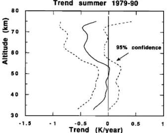
As mentioned earlier, tile c•l•fidence interval in the

15,308 Hauchecorne et al.' Rayleigh Lidar Temperature Climatology number of data. As an exat•l,le, Ihc linear trend obtained in

summer including 1990 data is prosculled in Figure A I. It

confirms the results presenlcd in !:igurc 6b t'or the 1979-1989 period, but the negative tre•tl observed in the mesosphere is now significant at the 95% co•t'idcnce level in the interval 57-

72 km. 80 •60 50 40 30 Trend summer 1979-90 I I I ' 95% confidence

-

Fig. A1. Linear trend of the !idar temperature during summer

months (data from 1979 to 1990).

Rclbrences

Aikin, A. C., M. L. Chanin, J. Nash and D. J. Kendig,

Temperature trends in Ihc lower mesosphere, Geot>hvs.

Res. Lett., 18,416-419, 1991.

Angell, J.K., Rocketsonde evidence for a stratospheric

temperature decrease in the western hemisphere during

1973-1985, Mon. Weather Rev., 11,5, 2569-2577, 1987.

Barnett, J. J., and M. Corney, Middle atmosphere reference

model derived from satellite data, Handbook for Middle

Atmosphere Program, 16, 47-137, 1985.

Brasseur, G., The response of the middle atmosphere to change in solar activity, in Our changing atmosphere,

1989, 21• Liege International Astrophysical Colloquium,

255-264, Universit6 de Lib•gc, (•'ointe-Ougree, 1989. Brasseur, G. and M. T. Hilchman, Stratospheric response to

trace gas perturbations: changes in ozone and temperature

distributions, Science, 240, 634-637, 1988.

Brtihl, C., and P. J. Crutzcn, Sce•tarios of possible changes in atmospheric temperatures and ozone concentrations due

to man's activities, esti•atecl with a one-dimensional

coupled photochemical cliohate •odel, Climate Dynamics,

2, 173-203, 1988.

Chanin M. L, A review of Ihe I I year solar cycle, the QBO

and the atmosphere relatitmship., !landbook for Middle

Atmosphere Pro_re'am, 22, 1989.

Chanin, M. L., and A. !!auchecorne, Lidar studies of

temperature and density using Rayleigh scattering, Handbook for Middle Atmosphere Program, 13, 87-99,

1984.

Chanin, M. L., P. Keckhut, A. Hauchecorne and K. Labitzke,

The solar activity-QBO effect in the lower thermosphere, Ann, O½•phys., 7, 463-470, 1989.

Clancy, R. T. and D. W. Rusch, Climatology and trends of mesospheric (58-90 kin) tc•nt)eratures based upon 1982- 1986 SME limb scattering profiles, J. Geophys. Res., 94,

3377-3393, 1989.

Curtis, P. D., J. T. Houghton, G. D. Peskett and C. D.

Rodgers, The pressure modulator radiometer for Nimbus

F, Proc. R. Soc. London. Set. A, 337, 135-150, 1974.

Drummond, J. R., J. T. !!oughton, G. D. Peskett, C. D. Rodgers, M. J. Wale, J. Whitney and E. J. Williamson, The stratospheric and mesospheric sounder on Nimbus 7,

Philos. Trans. R. Soc. London. Ser. A, 296, 219-241, 1980.

Ellis, P., G. Holah, J. T. Hougllton, T. S. Jones, G.

Peckham, G. D. Peskett, l). R. Pick, C. D. Rodgers, H.

Roscoe, R. Sandwell, Remote sounding of atmospheric

from satellites. IV: The selective chopper radiometer for

Nimbus 5, Proc. R. Soc. London. Ser. A, 334, 149-170, 1973.

Frederick, J. E., Measurement requirements for the detection

of ozone trends, Ozone correlative measurements

workshop, NASA Conf, Publ,, 2362, B1-B 19, 1984. Gadsen, M., A secular change in noctilucent cloud occurrence,

J. Atmos. Terr. Phys., 52, 247-251, 1990.

Garcia, R., S. Solomon, R. G. Robie and D. W. Rusch,

Numerical response of the middle atmosphere to the 11-

year solar cycle, Planet. St)ace Sci., 3,32.2, 411-423, 1984. Gille, J. C., J. M. Russell !!l, P. I•. Bailey, L. L. Gordley, E.

E. Remsberg, J. H. Lienesch, V. W. G. Planet, F. B. House, L. V. Lyjak and S. A. Beck, Validation of temperature retrievals obtained by the Lilb Infrared Monitor of the Stratosphere (LIMS) experiment on NIMBUS 7, J. Geophys. Res., 8{), 5147-5160, 1984.

Gille S.T., A. Hauchecorne and M. 1•. Chanin, Semidiurnal

and diurnal effects in the middle atmosphere as seen by lidar, J. Geophys. Res., 96, 7579-7587, 1991.

Hansen J., G. Russell, D. Rind, P. Stone, A. Lacis, A.

Lebedeff, R. Ruedy and L. '!'rayis, Efficient three- dimensional global models for cli•nate studies: Models I

and II, Mon. Weather Rev,, 1 11,609-662, 1983.

Hauchecorne, A. and M. L. Chanin, Density and temperature

profiles obtained by lidar between 35 and 70 km,

Geophys. Res. Lett., 7, 565-568, 1980.

Hauchecorne, A. and M. L. Chanin, Mid-latitude Lidar

observations of planetary waves in the middle atmosphere

during the winter of 198 I-1982, J. Geophys. Res., 88,

3843-3849, 1983.

Hauchecorne, A., M. L. Chanin and R. Wilson, Mesospheric

temperature inversion and gravity wave breaking, Geophys. Res. Letters, 14,933-936, 1987.

Hauchecorne, A. and A. Maillard, A 2-I) dynamical model of

mesospheric temperature inversions in winter, Geophys.

Res. Letters, 17. 2197-22(}0, 1990.

Keckhut, P.and M. L. Chani•, Seasonal variation of the 11

year solar effect on the •niddlc atmosphere; role of the QBO, Handbook for Middle Atmosohere Program, 29,

33-38, 1989.

Labitzke, K. and M. L. Chanin, Changes in the middle atmosphere in winter related to the I 1-year solar cycle, Ann. Geophys., fi, 643-644, 1988.

Labitzke, K., G. Brasscur, B. Naujokat and A. De Rudder, Long term temperature trends in the stratosphere: possible influence of anthropogenic gases, Geor•hvs. Res. Letters.

13, 52-55, 1986.

Labitzke, K. and H. van Loon, Association between the 11-

year solar cycle and the atmosphere. Part I' the

troposphere and stratosphere on the northern hemisphere

in winter, J. Arm. Tcrr, ph. ys,, 50, 197-206, 1988.

Lefr•re, J., J. Pelon, C. Caren, A. Hauchecorne and P.

Flamant, Survey of the post Mr. St. Helens stratospheric

aerosol at Haute-Provence Observatory, Appl. Opt., 7,

A70, 1981.

Miller, D. E., J. L. Brownscombe, G. P. Carruthers, D. R.

Pick and K. H. Stewart, Operational temperature sounding

of the stratosphere, Philos. Trans. R. Soc. London. Ser.

A, 296, 65-71, 1980.

Mohanakumar, K., Influence of solar activity on middle

atmosphere associated with phases of equatorial QBO,

)

Handbook for Middle At•nosphere I rogram, 29, 39-42,