Contents lists available atScienceDirect
Energy Conversion and Management: X
journal homepage:www.journals.elsevier.com/energy-conversion-and-management-x
Impact of Power-to-Gas on distribution systems with large renewable energy
penetration
Andrea Mazza
a,⁎, Fabio Salomone
b, Francesco Arrigo
a, Samir Bensaid
b, Ettore Bompard
a,
Gianfranco Chicco
aaDipartimento Energia “Galileo Ferraris”, Politecnico di Torino, Corso Duca degli Abruzzi 24, 10129 Torino, Italy bDipartimento di Scienze Applicate e Tecnologia, Politecnico di Torino, Corso Duca degli Abruzzi 24, 10129 Torino, Italy
A R T I C L E I N F O Keywords:
Distribution system Energy transition Power-to-Gas
Renewable energy sources Storage
A B S T R A C T
The exploitation of the Power-to-Gas (PtG) technology can properly support the distribution system operation in case of large penetration of Renewable Energy Sources (RES). This paper addresses the impact of the PtG op-eration on the electrical distribution systems. A novel model of the PtG plant has been created to be re-presentative of the entire process chain, as well as to be compatible with network calculations. The structure of the model with the corresponding parameters has been defined and validated on the basis of measurements gathered on a real plant. The PtG impact on the distribution systems has then been simulated on two network models representing a rural and a semi-urban environment, respectively. The testing has been carried out by defining a set of cases that contain critical situations for the distribution network, caused by RES plant place-ment. The objectives of the introduction of PtG are the reduction of the reverse power flow, as well as the reduction of the overcurrent and overvoltage issues in the distribution system. The results obtained from annual simulations lead to considerable reduction (from 78 to 100%) of the reverse power flow with respect to the base case, and to alleviating (or even solving) the overcurrent and overvoltage problems of the networks. These results indicate PtG as a possible solution for guaranteeing a smooth transition towards decarbonized energy systems. The capacity factors of the PtG plants largely vary depending on the network topology, the RES pe-netration, the number of the PtG plants and their sizes. From the test cases, the performance in a rural network (where the minimum capacity factor is about 50%) resulted better than in a semi-urban network (where the capacity factor values range between 21% and 60%).
1. Introduction
In the last years, the increase of Renewable Energy Sources (RES) has changed the paradigm of the distribution system operation, by imposing a shift from the traditional case of a completely passive net-work to a more and more active netnet-work hosting an increasing share of local generation. The local generation is variable during time and can create different issues, such as i) reverse power flow (occurring when the distribution system injects power into the transmission system), and ii) operational constraint violations (in terms of voltage and current limits). For solving these problems without the RES production cur-tailment, the excess of local generation should be converted and stored in appropriate forms.
The choice of the type of storage to be used depends on the need to use more power (generally with relatively short duration) or more en-ergy (from equipment that guarantee longer autonomy). Power-to-Gas
(PtG) is a solution that can exploit the excess of electricity from the local generation system to produce and store gas, then using the stored gas at a later time for different purposes. These characteristics make PtG adapt to be integrated into multi-energy systems [1,2] and to participate in the energy system operation in a flexible way[3].
In general, PtG plants can be divided into two main product chains:
•
Power-to-Hydrogen, where the excess of electricity from RES istransformed in hydrogen[4]
•
Power-to-Methane, where the hydrogen produced is converted inmethane through methanation[5]
This paper focuses on the second production chain and aims to study the integration of a PtG plant into a high-RES distribution system.
In the literature, there are relatively few studies that combine both PtG and distribution systems. In[6], the authors have investigated the
https://doi.org/10.1016/j.ecmx.2020.100053
Received 22 December 2019; Received in revised form 23 June 2020; Accepted 14 July 2020
⁎Corresponding author.
E-mail address:andrea.mazza@polito.it(A. Mazza).
Available online 18 July 2020
2590-1745/ © 2020 The Authors. Published by Elsevier Ltd. This is an open access article under the CC BY-NC-ND license (http://creativecommons.org/licenses/BY-NC-ND/4.0/).
use of an electrolyser as an alternative for network expansion in case of high photovoltaic (PV) penetration. A real network has been modelled and the size of the electrolyser has been obtained by considering the same effect reached by cable substitution. The techno-economic ana-lysis has highlighted that the profitability is greatly depending on the local excess of RES[7]. More in detail, RES electric excess has been used for sizing of the PtG plant capacity, reaching an overall PtG plant efficiency of about 77% (on a LHV basis) and a utilization factor of about 30%[7]. These results have been obtained both optimising the thermal integration between the methanation unit and the electrolyser, and analysing the management of each equipment[7]. The use of a low-voltage (LV) electrolyser has been studied by predicting the tem-poral variation of excess energy occurring in low voltage networks at 2030 and by identifying appropriate electrolyser capacities, while not considering any network topologies, but only an equivalent energy balance at a single node[8]. In[9], the mitigation effect of electrolysers on the reverse power flow has been exemplified on a LV grid. The evaluation of the use of power-to-methane chain in case of distribution systems characterised by an excess of wind production has been ana-lysed in[10]. The study has been based on the consumption of gas and electricity of a local area, and the use of combined heat and power (CHP) plants locally installed has been considered as well. In[11], the authors have focused on voltage regulation in active power distribution systems, by presenting a new algorithm for the real time scheduling of PtG and Gas-to-Power (GtP) plants by considering also arbitrage op-portunities. In [12], the authors have presented a voltage control strategy by coordinating both the On-Load Tap Changer and an alkaline electrolyser modelled dynamically as in [13]. The same electrolyser model has been used in[14]for studying how the electrolyser can be optimally designed and installed for facing the increase of RES in future active distribution networks. The alleviation of reverse power flow, line congestions and power losses in integrated power and gas network has been studied in[15–17], respectively. In those cases, the authors have presented three different scheduling algorithms to properly deploy power-to-methane and GtP conversion unit for distribution network support. The constraints of the chemical plants have been represented in terms of minimum and maximum power and gas flow of the plants. All the above papers have modelled the PtG units as “black boxes” without considering the physical connections existing among the dif-ferent plant parts, and thus also auxiliary services (such as compression systems) have been missed by the modelling aspects. Thanks to the multi-disciplinary team composing the project STORE&GO [18], the complete model of a PtG plant1has been created and then included in a
power flow calculation. For representing the effect on different seasons, the annual irradiation profiles have been considered with reference to the installation sites of the demonstration plants of the project. Fur-thermore, for understanding the effect on different network topologies, two realistic network models have been introduced to show the effect on both rural and semi-urban grids. Typical load profiles have been included to represent the variability of the loads in time. Great atten-tion has been devoted to the case study creaatten-tion, by considering dif-ferent possible positions of the PV plants in the grid.
Regarding the electrical point of view, the PtG plant is a particular type of load, and as such it has to be properly modelled in a power flow calculation tool. PtG plant modelling is an open research issue, espe-cially because of the need of providing a sound validation of the model on the basis of real case applications. On the basis of the previous considerations, this paper presents a number of specific contributions to the modelling and exploitation of PtG in distribution systems, namely: 1. The PtG plant modelling is addressed in order to formulate a steady-state model of PtG to be incorporated in the power flow equation
solvers. The validation of the model is carried out on the basis of measurements collected from a real PtG plant.
2. The impact of PtG on the distribution system operation is then studied through simulations in steady-state conditions. Different loading and RES penetration are considered for reproducing dif-ferent network issues that may be alleviated by using PtG plants. Dedicated cases are created with different RES penetration, by lo-cating the RES sources at network nodes that correspond to critical conditions for the amount of reverse power flows, as well as for the presence of overcurrent and overvoltage issues in the distribution network.
The rest of the paper is organised as follows.Section 2presents the characteristics of the PtG plant modelled and highlights the modularity of the proposed model.Section 3focuses on the creation of the case studies, by considering different PV penetration and location in the two networks.Section 4shows the results, whereasSection 5provides the concluding remarks.
2. PtG plant model
The PtG plant consists of a low temperature-based electrolyser (LTE), a buffer and a methanation unit. A simplified scheme of the PtG process is illustrated in Fig. 1. The LTE converts liquid water into gaseous oxygen at the anode and gaseous hydrogen at the cathode through electrolysis [7,19–22]. According to the literature, the effi-ciency of the electrolysis ranges between 55% and 70% (on a LHV basis) [7,23,24]. The hydrogen produced within the LTE could be stored in a tank or sent to the methanation unit. The hydrogen is mixed in stoichiometric ratio with carbon dioxide (H2/CO2molar ratio equal
to 4) in order to supply the methanation unit that produces synthetic natural gas (SNG)[7,19,22].
In addition, the main characteristics of the PtG are summarized in Table 1.
2.1. Characteristics of the electrolyser
A low temperature-based electrolyser is characterised by a power-to-hydrogen efficiency, whereas the methanation unit is characterised by a certain value of the CO2 conversion efficiency (i.e., 98.5%
[7,19,25]).
The PtG model has been built considering the dynamics (start-ups, shutdowns and partial loads) of a real plant installed in the demon-stration site of Falkenhagen (Germany), whose process is based on Alkaline Electrolysis (AEC). This plant consists of a 2 MW AEC-elec-trolyser, which was composed of 6 AEC modules (330 kW each one). The electrolysis technology considered has minimum loadPMIN= 20% [23]and power-to-hydrogen efficiency ηH2= 57.6%2(real data).
The characteristics of minimum load and efficiency of the AEC technology has been directly provided by the Falkenhagen plant man-agers, based on their long-time experience in the plant operation. It is worth noting that the AEC efficiency is in line with the related literature [24,26]. Regarding the minimum load of the electrolyser (i.e., the power to be provided for producing the minimum amount of H2), the
values existing in the literature are even lower than 20% but they may lead to problems (see for example[23,27]). The modularity of these technologies simplifies the management of the electrolyser, moreover each module could be maintained in hot stand-by if there is not enough electrical energy for supplying the PtG plant.
On the one hand, the electrolyser has a wide rangeability thanks to its modularity. On the other hand, the methanation reactors have a narrow rangeability due to the kinetics of the methanation reaction [25,28]. More specifically, according to the literature[25], the reactors
1From this point, with PtG plant only the power-to-methane chain will be
are conceived as tube-bundles refrigerated by evaporating water at 250 °C. The methanation reaction is extremely exothermic [28,29]; hence, the tube diameter must be small for avoiding too high radial thermal profiles. Obviously, the design of a methanation reactor is made for the nominal productivity; however, the residence time in-creases (and the gas hourly space velocity dein-creases) reducing the productivity. Consequently, the heat generation profile along the axis of the reactor becomes narrower and more intense; in addition, the overall heat exchange coefficient decreases[19,25]. Therefore, it could cause problems of thermal management, hot spots and local deactivation of the Ni/γ-Al2O3catalyst (i.e. sintering)[7,28–30]. Hence, each reactor
could be parallelized in 3 or 4 bundles in order to increase the range-ability of the PtG plant, for instance, from about 60–110% (i.e., only one bundle for each reactor) to about 20–110% (i.e., three bundles in parallel for each reactor). For all these reasons, the best option is to maintain the methanation unit at least at the minimum operative load. The model developed in this work, as additional feature, considers also all the auxiliary consumptions, which can be easily adjusted ac-cording to the actual PtG plant layout. More in detail, the energy consumption of a compressor (Ecompr, W) was calculated according to
Eq.(1) [31], where Z is the compressibility factor that was assumed unitary, R (8.314 J mol−1K−1) is the ideal gas constant, T
in(K) is the
inlet temperature, nin(mol s−1) is the inlet molar flow rate, γ is the heat
capacity ratio, and ηcompris the compression efficiency, which was set
equal to 70% and pinand poutrepresent the inlet and outlet pressure,
respectively. In addition, multistage compression was considered if the compression ratio (pout/pin) was greater than 4.
=
E Z R T p
p n
· · · ·
1 · 1 ·
compr in compr out
in
in
1 · compr
(1) Moreover, the methanation unit and the electrolyser require an additional electric consumption due to heat dissipations caused by natural convection[7], if they are maintained in hot stand-by.
2.2. The electrolyser model
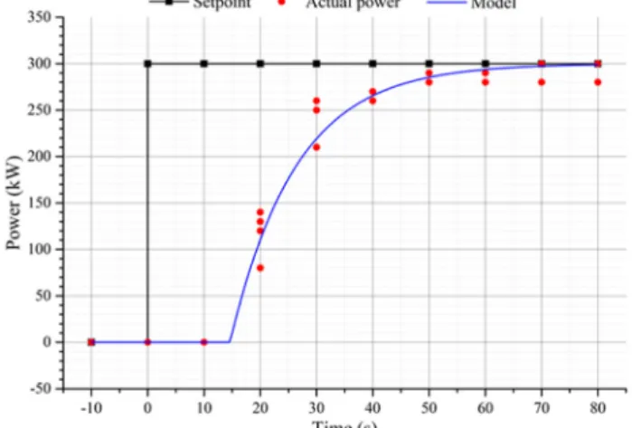
The dynamic behaviour of the AEC-electrolyser has been obtained from the analysis of a test carried out at the Falkenhagen plant (shown inFig. 2).
The test had duration of about 11.5 h and highlighted that the AEC-based electrolyser had a fast response when the setpoint changed. Therefore, its response could be modelled for the purpose of forecasting the behaviour of the AEC-based electrolyser when it is coupled with an intermittent RES-based electrical profile. It is worth mentioning that during the test, the set point of the electrolyser was periodically
Fig. 1. Simplified low temperature-based Power-to-Gas process scheme considering H2storage. Table 1
Characteristics of the PtG plant.
Parameter Value Parameter Value
LTE operating temperature 80 °C CO2conversion within the methanation unit 98.5% LTE and methanation unit pressure 15 bar Inlet – outlet temperature of the cooling water 28 – 32 °C H2tank maximum pressure 60 bar Coolant temperature in the methanation unit 250 °C
changed with steps of different amplitude to explore a large number of operating conditions.
The easiest model to describe the AEC-based electrolyser behaviour is a first order system with delay, which is characterised by three parameters; the mathematical model of its response to a step is de-scribed by means of Eq.(2) [32–34]:
= = <
(
)
y t y t A K ( ) 0 ( ) 1 exp If t If t t (2) In this equation, y t() is the actual power of the AEC-based elec-trolyser (MW) at the time stept(s), A is the step amplitude of the set point (MW), K is the gain of the system, is the time delay of the response (s), is the time constant of the system (s). The gainKcan be evaluated by means of Eq.(3), where y( ) is the actual power of the electrolyser after a large period of time (stationary condition):=
K y
A
( )
(3) The two time parameters ( and ) have been estimated by means of the Sundaresan and Krishnaswamy’s method[35], according to Eqs.(4) and (5), respectively. The two parameters were calculated using two characteristic points of the response curve: t1 represents the time in which the response reaches 35.3% of the stationary value y( ), while t2 is estimated as the time in which the response reaches 85.3% of the final value y( ):
=1.3t1 0.29t2 (4)
=0.67 (t2 t1) (5)
For the purpose of evaluating these three parameters, four steps with the same amplitude (i.e., 0.3 MW) have been considered, by ob-taining the parameters shown inTable 2. These steps are highlighted in Fig. 2between 40 min and 100 min of the test.
The fit between the model output and the real data is shown in Fig. 3.
2.3. Simulation algorithm of the PtG plant model
The flowchart of the simulation algorithm (called in the sequel
function_PtG) is shown inFig. 4.
The simulation algorithm consists of the following main instruc-tions:
•
Setpoint: the setpoint is defined as the theoretical maximumopera-tive power at which the electrolyser may work. This maximum can correspond to either the power provided by the grid (when it is lower than the nominal power of the electrolyser) or the nominal power of the electrolyser (in the case it exceeds the nominal power of the electrolyser).
•
Actual power: it represents the actual electric consumption that couldbe calculated using the dynamic model of the AEC-based electro-lyser (Section 2.2).
•
Hydrogen production: the hydrogen flow could be evaluated takinginto account the efficiency of the electrolyser.
•
Hydrogen tank management: if the electrolyser is operative, aminimum hydrogen flow feeds the methanation unit. Beyond this, certain amount of hydrogen is sent to a hydrogen tank until the tank is completely full (the priority is filling the tank). This operation allows to decouple the methanation unit from the electrolyser. When the electrolyser is not operative, the stored hydrogen is fed to the methanation unit, for producing continuously SNG. In this case, the methanation unit works at the minimum power load; when the hydrogen tank is completely empty, it could be turned off and
Fig. 2. Falkenhagen test on an AEC-based electrolyser.
Table 2
Characteristics of the low temperature-based electrolyser.
Parameter Value
K 1
[s] 14.62
[s] 11.73
Fig. 3. AEC-based electrolyser response model estimated using Falkenhagen
test data (first order system with delay). It is worth noting that the experimental data (red spots) refer to the four steps considered for the modeling, as men-tioned in the text. For comparing the behavior of the response, the starting values of the real steps were shifted to zero (baseline), and thus some data are overlapping.
remain in hot standby conditions3. More in detail, H
2produced in
the LTE could be split into two streams. During the filling of the H2
tank three configurations have to be considered:
♦If the H2tank is empty, its pressure is lower than the operative pressure of both the LTE and the methanation unit. Therefore, the compressor (P-102) is useless and the H2tank could be partially
filled using stream 9 until the storage pressure is equal to the operative pressure of the LTE.
♦If the H2tank is partially filled, its pressure ranges between the
operative pressure of the LTE and the maximum storage pressure. Therefore, the compressor (P-102) is used for filling the tank until it is completely full.
♦If the H2tank is completely full, the produced H2is directly fed to the methanation unit using stream 16.
•
If the LTE does not produce H2, the methanation unit could be fedusing the stored H2. In this case, three configurations could be
possible:
♦If the tank pressure is higher than the operative pressure of the methanation unit, H2 could be fed to the methanation unit
through stream 14.
♦If the tank is emptying, H2could be fed to the methanation unit
using the compressor P-103 until the tank is completely empty. ♦If the H2tank is empty and no electricity is available for
produ-cing H2, the methanation unit must be turned off (shutdown of
the PtG plant).
•
Auxiliary consumptions: all the consumptions of the auxiliary items ofequipment are related to the amount of produced hydrogen. Firstly, the hydrogen could be compressed; secondly, the carbon dioxide has to be compressed; thirdly, the water has to be pumped and lastly it must be heated up to the temperature of the electrolyser.
•
Control of the setpoint: the setpoint power of the electrolyser must berecalculated considering the new auxiliary consumptions, because the available electricity is comparable with the power absorbed by the electrolyser. This affects the power withdrawn from the power grid.
•
Methanation unit: the amount of SNG could be calculated using theCO2conversion, or alternatively, the hydrogen-to-SNG efficiency.
3. Creation of the case studies
As widely shown in literature (for example in[36]), the installation of large share of RES can create the following issues in the electrical networks:
•
Reverse power flow (RPF): on the one hand, a reverse power flowaffects the transmission system because the point of connection between transmission and distribution system becomes equivalent to a non-controllable active node. On the other hand, the presence of reverse power flow can create issues also at the distribution system, for example in terms of not proper protection schemes. Usually, these problems are nowadays solved by cutting the excess of pro-duction or using some pilot battery-based storage[37].
•
Overcurrent (OC): the large share of RES can create overcurrentsalong the feeders. These overcurrents can affect only a portion of the network (e.g., the last portion) or the entire network, depending on
Fig. 4. Flowchart of the algorithm (function_PtG).
3A hot standby condition (it means that the equipment is maintained at the
operative temperature conditions with auxiliary energy, in order to ensure a fast start up) was assumed for the main equipment (electrolyser and metha-nation unit).
the level of load and distributed generation, together with the geographical position of the PV plants.
•
Overvoltages (OV): this problem is characteristic especially of ruralnetworks, composed of long feeders (also up to 10 km), and char-acterized by a high R/X ratio, which leads to have to voltage level changes strictly linked with the active power flowing in the grid branches.
It is worth noting that the presence of reverse power flow leads to the network operating in an alert condition, whereas the presence of over-current and overvoltage are symptoms of an emergency condition (be-cause directly affecting the operational constraints of the network)[38]. Hence, the distribution system operators needs to solve these problems as soon as possible, by making use of different approaches which can even result in lower quality of service (e.g., load disconnections). So, the si-mulations carried out starting from conditions in which the network constraints are not satisfied (even though these conditions do not cor-respond to real situations) have the goal to show, in very extreme cases, how the potential use of PtG can alleviate these problems as well.
The creation of the case studies needs the proper placement of the PV plants. In this study, the placement of the PV plants has been carried out by using two different approaches:
•
Topological approach: the PV plants have been installed according tothe length of the network lines.
•
Losses Allocation Factors-based approach: in this case, the approachshown in [39]and based on [40]has been adopted. A detailed analysis on the implication of the use of the loss allocation for dis-tribution system analysis can be found in[41].
These approaches are followed by using a series of assumptions on the model of the distribution system, namely, (i) the power flow is calculated as an equivalent single-phase circuit. This is justified in medium voltage networks (to which PtG is connected, because of its size), where loads and generations are usually distributed in a relatively uniform way on the three phases; (ii) the distribution system is analysed in time as a succession of steady state conditions, in which constant
average power withdrawn/injected by loads and local generations in every time step are considered for the power flow calculations. This also implies that the frequency is considered constant (at 50 Hz) during the entire simulation horizon. The use of more detailed dynamic models for the electrical system, which would be able to represent real-time phe-nomena at milliseconds to seconds scale, is not needed for the type of analysis carried out in this paper; and (iii) the network parameters are known and constant during the entire simulation horizon, which is a usual assumption made in the power flow calculations. This implies that external conditions (such as temperature, etc.) do not affect the para-meters (e.g., loads or branch resistances).
3.1. The network samples
This work considers two network samples:
•
Semi-urban network, adapted from the one shown in[42], by adding time-varying loads with different profiles. For this network only the topological PV placement has been applied[43].•
Rural network, developed in the project Atlantide [44]. For this network, both PV placement methods have been used.The two network samples aim to represent different network topologies and allow to emulate the distribution systems in the areas where the demo sites of the project are installed. The two demo sites are installed in Solothurn (Switzerland) and in Troia (Italy). In particular, the semi-urban network refers to Solothurn area, whereas the rural network refers to Troia area.
Few samples referring to daily PV profiles in different months for the two networks are shown inFig. 5, whereas the load profiles are shown inFig. 6. It is worth noting that the PV profiles are different for the two network samples because referring to two different geographic locations, and have been obtained from[45].
Moreover, during the night time the PtG plant is supplied by the main grid to guarantee the continuous operation of the plant in com-pliance with its minimum power specified in Section 2.1 (i.e.,
PMIN= 20%).
Fig. 5. PV profiles considered for building the case studies. Four months have been considered (January, April, July and October): (a) semi-urban network and (b)
rural network.
3.2. Introduction of the PtG plant model into the calculation loop of the network operation
The model of the PtG explained inSection 2needs to be integrated in the network solver, which is based on the Backward Forward Sweep (BFS) method[46]. The response of the PtG unit is modelled as a first order system and solved through the Matlab®-embedded solver ode45. The calculation loop is shown inFig. 7. The variables used in the cal-culation loop are presented inTable 3.
After having loaded the inputs, the algorithm runs the BFS for the
first time: this is requested for defining the network conditions (i.e., nodal voltages and branch currents). On the basis of this, the h-th column of the matrix RPF (containing the value of RPF at every branch the interaction h) is updated. At the same time, the h-th columns of both matrices OV and OC are updated with the values of overvoltage and overcurrent, respectively. On the basis of the above values, a compound
set pointPPtG_set[ ]h is produced, and is referred to the RPF and
over-current value of the branch upstream with respect to the node of the PtG plant, while the contribution regarding the overvoltage is linked to the overvoltage value of the node where the PtG plant has been in-stalled as presented in Eq.(6), i.e.:
=
h f h h h
PPtG_set[ ] (RPF[ ],OV[ ],OC[ ]) (6)
In particular, the different set point components are set as follows:
•
Component referring to the RPF: this component is equal to value ofpower needed for eliminating the reverse power flow in the up-stream branch with respect to the node where the PtG plant is in-stalled.
•
Component referring to the OC: this component is equal to the value ofpower that, absorbed from the PtG plant, would help to reduce (at 80% of the thermal limit) the current flowing in the upstream branch with respect to the node where the PtG plant is installed.
•
Component referring to the OV: this component is equal to the value ofpower that, absorbed from the PtG plant, would help to reduce (at 1.05 pu) the voltage of the node where the PtG plant is installed.
3.3. Installation and sizing of the PtG plants
The study of the impact of the PtG plants on the distribution system requires to i) choose the node where the plants are installed and ii) their sizes. These two elements are requested by the calculation loop shown inFig. 7, and in this work have been solved by applying the Simulated Annealing (SA) method[47]. It is worth noting that the main goal of this paper is not introducing a new algorithm for the siting and sizing of the PtG plants, but creating meaningful case studies to get insights re-garding the impact of the PtG plants on distribution system operation. However, the step regarding the siting and sizing is requested as pre-liminary task, for emulating the process that, in the future, could bring to rationally install a defined number of MW-scale PtG plants. Few notes regarding the use of the SA in this work are reported in Appendix. The objective functions used in the algorithm have as main variables the value of reverse power flow, overcurrent and overvoltage of the network. In particular, the network with the installed PtG plants (de-noted as X) can be affected by:
•
Only reverse power flow•
Reverse power flow and overcurrent•
Reverse power flow and overvoltage•
The combination of the last two casesFig. 7. The main calculation loop of the distribution system. The function called
function_PtG represents the PtG complete model.
Table 3
Input parameters of the main calculation loop.
Inputs Description
Ntime_steps Number of time steps of the analysis
PtG data Number of the PtG plants NPtG_plants, their positions (indicated by the nodes contained in the set NPtG) and their sizes
H2, tank(0) Initial value of the matrix of dimensions {NPtG_plants, Ntime_steps} representing the volume of H2in the tank in time Nkeep_steps Number of points for running PtG model
Network data Set of the network nodes J, set od the network branches B, number of nodes Nnodes, number of branches Nbranches, line parameters, incidence matrix, rate nodal power, lines thermal limits
Load and generation profiles Load and generation profiles for evaluating the initial value of the matrix Snet(0), i.e., the net nodal power (dimensions {Nnodes, Ntime_steps}) RPF Matrix of dimensions {Nbranches, Ntime_steps} containing the value of reverse power flow at every time step
OC Matrix of dimensions {Nbranches, Ntime_steps} containing the value of overcurrent for every branch during the time span of simulation OV Matrix of dimensions {Nbranches, Ntime_steps} containing the value of overvoltages for every node during the time span of simulation PPtG_set Matrix of dimensions {NPtG_plants, Ntime_steps} containing the set points of the PtG plants
All the cases make use of a penalised objective function where the constraints of the problem are integrated within the objective function through penalisation factors indicated with the Greek letter . This approach allows driving the optimisation towards solution with no constraint violations. In particular, the operational constraints are the voltages Vj of the network nodes and the currents Ib flowing in the network branches, which have to remain inside the following ranges:
•
Vj(min)≤ Vj≤ Vj(max), with j J, whereJdenotes the set of nodes. The node voltage is usually expressed in per unit (pu) with respect to the nominal voltage (i.e., Vj= 1 means that the voltage value of the node j is equal to the nominal voltage of the system). Usual values of the extremes of the range areVj(min)=0.9pu andVj(max)=1.1pu.•
Ib≤ Ib( ,th max), withb B, where B denotes the set of branches. The value of Ib( ,th max)is strictly depending on the conductors installed. The objective function at the iteration k of the method in case of existence of the sole reverse power flow is shown in Eq.(7):The penalised objective function at the iteration k is expressed in pu with respect to the value of the reverse power flow in the initial con-figuration. The reverse power flow is evaluated here through the number of minutes in which it is present during the entire period of analysis. The formulation penalises (through the factors V and I) all the configurations that do not respect the operational constraints (i.e., maximum and minimum voltage, and thermal limits) of the network. Thus, the constraints of the objective function(7)are the operational constraints of the network Vj(max), Vj(min) and Ib( ,th max), for node j and branch b, respectively. For every node/branch the worst condition (e.g., the maximum current Ib(worst)during the day) is chosen as representative value to force the worst condition respecting the imposed constraint.
When both overcurrent and reverse power flow exist in the initial configuration, the objective function is modified as reported in Eq.(8):
In this case, the objective function is still expressed in pu with re-spect to the initial configuration. The normalised sum of the minute of overcurrent and the minute of reverse power flow during the entire time horizon are modified according to the product of the penalty factors and the value of the constraint violation. In this case, the con-straints are the maximum and the minimum voltage values, indicated as
Vj(max)and V
j(min), respectively.
The objective function in case both overvoltage and reverse power flow exist is shown in Eq.(9)and differs with respect to Eq.(8)only for the constraints considered, i.e., related to the branch thermal limits
Ib( ,th max)and the minimum nodal voltages Vj(min):
When all the issues listed above (i.e., reverse power flow, over-voltages and overcurrents) affect the grid, then the objective function is changed to solve them, as shown in Eq.(10):
= + + + f RPF RPF OV OV OC OC V V V X ( ) 1 k k k k j V j min jworst jmin J 0 0 0 ( ) ( ) ( ) 2 (10) It is worth noting that in Eq.(10)the constraint related to the minimum voltage value is still considered as part of the penalized objective function, to avoid that the worst value reached by the voltages in the period under analysis Vj(worst)falls below the minimum allowed value Vj(min).
As the final comment, the above objective functions are chosen a
priori according to the network issues that affect the distribution system
under analysis.
4. Results and discussion 4.1. Annual simulation
4.1.1. Network performance indexes
Different PV penetrations have been assumed for the creation of the case studies. The penetration has been calculated in terms of share of the
energy provided by the PV plants with respect to the system passive load
considering the PV production in July. In the case with 40% of PV penetration, the production in July covers 40% of the passive load. According to this, the PV penetration in other months varies following the different PV profiles.
The considered case studies and the existing problems in the dif-ferent cases are shown inTables 4and5for the semi-urban network and the rural network, respectively. The tables show entries different from zeros when that kind of problem exists, and the entry indicates the magnitude of the problem. The label “Pre” in the table indicates the magnitude of the problem without PtG installed, whereas the label “Post” refers to the condition when PtG plants have been installed. The RPF has been indicated in MWh, whereas the OC and OV are expressed in minutes.
The values refer to annual simulations. The two tables show the number of plants installed and, only for the rural network, the size of the plants as well. Due to the large number of plants installed in the case of semi-urban network, the sizes of the plants are summarised in Fig. 8.
First of all, it is evident that, while in the rural network is possible to obtain cases with problems of overvoltages and reverse power flow, in the semi-urban network is difficult to decouple overvoltage and over-current. This is linked with the nature of the lines composing the net-work, which are highly resistive for the rural network because mostly composed of long overhead lines.
It is worth noting that, as demonstrated through the rural network, the reverse power flow issue is not strictly linked to overvoltage pro-blems, but these two aspects can be decoupled through a suitable
= + + + f RPF RPF V V V V V V I I I X ( ) 1 k k j V j max jworst jmax j V j min jworst jmin b I b th max bworst bmax J J B 0 ( ) ( ) ( ) 2 ( ) ( ) ( ) 2 ( , ) ( ) ( ) 2 (7) = + + + f RPF RPF OC OC V V V V V V X ( ) 1 k k k j V jmax jworst jmax j V jmin jworst jmin J J 0 0 ( ) ( ) ( ) 2 ( ) ( ) ( ) 2 (8) = + + + f RPF RPF OV OV V V V I I I X ( ) 1 k k k j V jmin jworst jmin b I bth max bworst bmax J B 0 0 ( ) ( ) ( ) 2 ( , ) ( ) ( ) 2 (9)
installation of PV generation (as the one guaranteed by the procedure shown in[39]).
From the two tables it is evident that the deployment of PtG has a positive impact on alleviating the grid issues.
For the semi-urban network, in the cases in which the PV is installed at the end of lines with length L lying in the range 0 < L ≤ 0.45 km, the impact of PtG is indeed powerful, because both cases reveal how the reverse power flow can be strongly reduced: in fact, in case of PV pe-netration equal to 40% the reduction is over 99.9% (passing from al-most 11.3 GWh to 9.37 MWh), whereas with PV penetration equal to 80% the reduction is almost 78% (passing from almost 152 GWh to 34 GWh). In the cases with PV plants installed at the end of lines with length L lying in the range 0.5 ≤ L ≤ 3 km, the reduction of reverse power flow is stronger for lower PV penetration (more than 99.6% with PV penetration equal to 40%), but is anyway high also with PV pene-tration equal to 60% (the reverse power flow reduction reached almost 90%). Residual problems of overcurrents appear in all the cases except Case 1.
By analysing the worst case (i.e., the one with PV penetration equal to 60%), these issues affect in total thirteen branches, and the number of minutes in which the lines are overloaded lies between 4 and 5,456 min, whereas the maximum overload conditions at which they
operate lies in the range between 2.24% and 13.39%, as shown in Table 6. The system operator has to act for establishing again the proper network conditions, because the alleviation effect of the PtG deploy-ment cannot solve completely the overcurrent issues.
For the rural network, in the cases in which the PV is installed at the end of lines with length L lying in the range 0 < L ≤ 0.9 km, the impact of PtG is again powerful, because in one case (i.e., PV pene-tration equal to 40%) the reverse power flow is completely solved, whereas in the case with 80% of PV penetration the reverse power flow is strongly reduced, passing from 19,861 GWh to 1,633.9 MWh (re-duction of almost 92%). In the cases with PV plants installed at the end of lines with length L lying in the range 2 ≤ L ≤ 3, the reduction of reverse power flow is stronger in case of lower PV penetration (almost 100% with PV penetration equal to 40%), but is anyway high also with PV penetration equal to 80% (the reverse power flow reduction reached almost 83%).
Finally, the case created with the rural network by using the loss allocation shows that the reverse power flow problem can be solved in
Table 5
Case studies for the rural network.
Case Method PV placement Length*[km] PV penetration RPF [MWh] OC [min] OV [min] Number of PtG plants Size [MW] pre post pre post pre post
5 Topological 0 < L ≤ 0.9 40% 266.27 0 – – – – 1 2.5
6 80% 19,861 1633.9 165,047 0 504 – 4 2 (all)
7 2 ≤ L ≤ 3 40% 248.99 0.10 – – – – 1 2
8 80% 19,206 3,337.4 – – 276,329 0 4 2 (three plants) 1.5 (one plant)
9 Loss allocation – 40% 167.90 0 – – – – 2 2 (all)
10 80% 20,991 1868.4 – – – – 4 2 (all)
* The length refers to the branches of the MV network.
Fig. 8. Number and sizes of the PtG plants installed in the semi-urban network.
Table 6
Analysis of the overloaded lines in of semi-urban network, with 60% of PV penetration.
Lines overloaded Cumulative overload period
[min] Maximum overloading [%]
6 284 11.47 32 13 9.02 152 79 13.39 155 5,032 9.05 156 4,747 8.86 157 5,456 10.10 159 2,717 6.12 161 910 17.33 165 1,395 2.43 169 4,382 7.62 170 123 13.10 185 4 2.24 196 14 4.78 Table 4
Case studies for the semi-urban network.
Case number Length [km]* PV penetration RPF [MWh] OC [min] OV [min] Number of PtG plants
Pre Post Pre Post Pre post
1 0 < L ≤ 0.45 40% 11,298 9.37 – – – – 7
2 80% 151,920 33,654 90,616 35 – – 20
3 0.5 ≤ L ≤ 3 40% 10,213 31.4 430,087 6,978 3,356 0 12
4 60% 71,272 7,165 2,388,634 25,156 900,407 0 17
case of 40% of PV penetration, whereas a residual reverse power flow remains for the case 80% (but even in this case the reduction is more than 90%).
4.1.2. Capacity factors
The successful use of PtG plants needs a justification in terms of plant use, i.e., a capacity factor high enough.
The capacity factor Ci
f( )that refers to the i-th PtG unit is the ratio between the energy Ei
PtG( ) consumed by the i-th PtG unit during the si-mulation period tand the theoretical energy that the plant would be able to absorb during the same time period if it had consumed its nominal power; it was calculated according to Eq.(11):
= C E P t i i ni f( ) PtG ( ) ,PtG ( ) (11) where EPtG( )i is the energy consumed during the simulated time horizon
tby the i-th PtG plant, andPni ,PtG
( ) is the nominal power of the i-th PtG plant.
Fig. 9 shows the capacity factors for the semi-urban network. It shows that in Case 1 the plants result underused, and thus the number of plants chosen is too high. A reduction of the number of plants in-stalled could lead to a more fruitful use of the plants. In Case 2, only one plant results underused (i.e., having capacity factor equal to 23%), whereas the other plants are quite well exploited.
Case 3 presents 12 plants having a capacity factor lying in the range 40%–50%, whereas the remaining plants have a capacity factor be-tween 50% and 60%.
Finally, Case 4 presents three plants with capacity factor lower than 40% (i.e., from 28% to 37%), whereas all the other plants are well exploited (minimum about 51%).
From the results it is evident that the number of plants installed has a great impact and need to be carefully considered. The analysis carried out, in any case, neglects the presence of suitable gas network points: in the reality, the presence of real infrastructures will limit the potential nodes where PtG can be installed to a smaller number than the one considered here.
In the case of the rural network, the results are summarized inTable 7. With respect the previous case, the minimum capacity factor results higher than 60% in all the cases, and reaches almost 90% in one case. The results in the table indicate also for this case that PtG can handle very well the issues created from PV generation installed at the end of relatively long lines, by maintaining a sufficiently high capacity factor.
A good performance index of the network is the value of the power losses, which are summarized inTable 8.
The value of the losses (in MWh and in percentage) is reduced in all the cases. This reduction is obtained thanks to the installation of the plants that help to improve the network operation.
Another performance indicator is the voltage magnitude (maximum and minimum), whose values for both semi-urban and rural networks
are shown inTable 9. It is evident the effect of PtG to reduce the voltage at levels that are lying within the admissible ranges.
4.2. Network effect
This section aims to highlight the role of the network infrastructure in the proper evaluation of the effect of the PtG deployment.
In fact, some approaches existing in literature (e.g.,[7]) do not consider the existence of the electrical infrastructure, but only the po-tential unbalance between local generation and loads. However, this approach could not be proper for solving completely the issue caused by the excess of RES.
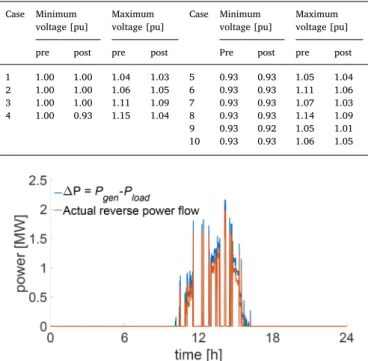
Taking as example a particular day of Case 54, the difference
be-tween generation and loads, without taking into account the network, is shown inFig. 10. The same figure also reports the actual reverse power flow existing in the network. The two curves are quite similar, but the first one overestimates the actual reverse power flow value.
For the sake of clarity, the rural network schematic is shown in Fig. 11.
The installation of plants characterised by different size at node 2 (connected to the network slack node) instead of node 83 (as in Case 5) leads to the results shown in Table 10. The solutions show that the
Fig. 9. Capacity factors for the different cases of semi-urban network. Table 7
Annual capacity factors for the rural network.
Case PV penetration Min capacity load [%] Max capacity load [%]
5 40% 47.55* – 6 80% 43.47 54.96 7 40% 47.104 – 8 80% 48.50 56.0 9 40% 43.07 49.26 10 80% 45.68 50.88
* These cases require only one PtG plant.
Table 8
Network losses for both the semi-urban network and the rural network.
Case Power Losses [MWh] Power Losses [%] Case Power Losses [MWh] Power Losses [%]
pre post Pre post pre post pre post
1 2,122.5 2,314.9 0.95 0.20 5 1,149.8 1,128.9 2.22 1.82 2 3,445.1 2,902.4 7.36 0.69 6 2,040.0 1,363.1 9.34 2.38 3 3,779.0 3,278.7 1.71 0.28 7 1,142.5 1,042.1 2.21 1.74 4 6,517.5 4,082.1 4.86 0.50 8 2,683.5 1,972.0 12.29 3.82 9 1,263.9 1,205.9 2.42 1.77 10 20,991 1,358.0 7.68 2.51
reverse power flow issue can be almost completely solved by using a plant with smaller size than the one referring at Case 5. This may lead to think that the solution of Case 5 could be not be optimal, because of the size. However, the capacity factor highlights that the installation of the plant at the node connected to the slack bus does not guarantee a good utilisation of the potential of the plant and thus the installation node should be carefully chosen. Furthermore, the use of the plant with
the position and size of Case 5 allows improving the network condi-tions, in terms of power losses and reverse power flow. This simple example aims to be an effective way to show the importance of the network information to capture all the aspects regarding the new op-eration of the electrical system when new devices are installed.
4.3. Response of the PtG model
The PtG model provides in output the following quantities:
•
Power profile sent by the control system to the electrolyser Pelec,sp•
Power profile of the electrolyser Pelec•
Power profile of the auxiliary services Paux,referring to i) the CO2compression system, ii) the circulation of H2O, iii) the compression
of the H2, and iv) the water heating.
•
The hydrogen flow rate sent to the tank φH2,tank[kmol/s]•
The hydrogen sent to the methanation unit directly from the elec-trolyser φH2, dir[kmol/s]•
The hydrogen sent to the methanation unit from the tank after compression φH2,tank,meth[kmol/s]•
The level of the hydrogen tank [%]•
The SNG produced seen as power profile [MW] or energy profile [MWh]With reference to the same day considered inSection 4.2of Case 5,
Pelec,sp, Pelecand Paux,are shown inFig. 12. InFig. 12(a), it is evident the
saturation imposed by the nominal power of the plant. Furthermore, the minimum power required by the AEC is different from zero and has to be provided by the main network.Fig. 12(b), instead, shows the power related to the auxiliary services. Three zones with different auxiliary service power exist, and each of them is characterized by different con-tributions, as highlighted inFig. 13. More specifically, during the night no excess of electrical power is available for the PtG plant; therefore, it operates at the minimum power load corresponding to 20% of the nominal installed power. As illustrated inFig. 13(a) auxiliary consump-tions are principally due to the CO2compression, while water pumping
and H2compression are marginal contributions. Subsequently, in the first Table 9
Minimum and Maximum voltage magnitude for both semi-urban and rural networks.
Case Minimum
voltage [pu] Maximumvoltage [pu] Case Minimumvoltage [pu] Maximumvoltage [pu] pre post pre post Pre post pre post 1 1.00 1.00 1.04 1.03 5 0.93 0.93 1.05 1.04 2 1.00 1.00 1.06 1.05 6 0.93 0.93 1.11 1.06 3 1.00 1.00 1.11 1.09 7 0.93 0.93 1.07 1.03 4 1.00 0.93 1.15 1.04 8 0.93 0.93 1.14 1.09 9 0.93 0.92 1.05 1.01 10 0.93 0.93 1.06 1.05
Fig. 10. Comparison between the actual reverse power flow (with and without
the network).
part of the day (between 6 h and 11 h) the electrical availability in-creases, and the electrolyser could work in its whole operative range (from 20% to 100%); thus, it produces a large amount of H2, which is
mainly stored in the tank until it is completely full. Hence, H2
com-pression represents 96% of all auxiliary consumptions, as shown in Fig. 13(b). At the same time, the methanation unit operates at the
minimum power load for allowing the tank to be filled: in fact, the CO2
compression represents 3% of the auxiliary consumptions even though it is the minimum power consumption for compressing CO2. Lastly, in the
second part of the day (between 11 h and 18 h), both the electrolyser and the methanation unit work in their whole operational range and the H2
tank is entirely full. More in detail, as depicted inFig. 13(c), H2has not to
be compressed and the CO2compression cost increases as the CO2flow
rises (H2and CO2are fed in stoichiometric ratio to the methanation unit).
Furthermore, all these aspects of the process are clearly illustrated in Fig. 14. As shown inFig. 14(a and b), the H2tank is filled during the first
hours of the day, when there is a large excess of electrical energy availability. Subsequently, both the electrolyser and the methanation unit operate for producing SNG, as depicted inFig. 14(b and c). In this case study (one day of Case 5), the alkaline electrolyser absorbs 28 MWh of electricity, which is converted into 237.4 kmol of H2(15.8 MWh, LHV
basis). Initially, the produced H2 is partially stored in the tank (50.9
kmol) until it is completely full; subsequently, the H2flow is sent to the
methanation unit for producing SNG (10.4 MWh, LHV basis). In this case study, the auxiliaries require 0.21 MWh of electrical energy during the whole day. It is worth noting that the tank is not discharged, because the minimum operative power set for the electrolyser was assumed to be
Table 10
Comparison between the network performance without PtG, with PtG installed without optimisation process and with optimisation process (referring to a day of Case 5). Size [MW] Reverse power flow [MWh] Reverse power flow [min] Power Losses [MWh] Power Losses [%] Capacity factor [%] 0 (no PtG) 2.16 151 3.08 2.29 – 0.5 1.026 143 3.09 2.24 50.81 1 0.284 139 3.096 2.20 44.21 1.5 0.062 135 3.102 2.17 36.02 2 0.025 120 3.108 2.14 30.44 2.5 0.022 110 3.114 2.11 27.03 2.5 (day of Case 5) 0 0 3.00 1.85 69.22
Fig. 12. Electrical quantities provided by the PtG model: (a) input power profiles and (b) power profile of the auxiliary services.
Fig. 13. Composition of the auxiliary services in the different periods of the day.
20% (as specified inSection 2), which is equal to the minimum flow required by the methanation unit. However, the model includes also the storage system, which can intervene if a different control is applied.
5. Conclusions
This paper has presented a detailed study regarding the impact of PtG technology on the electrical distribution system. The study takes into account both electrical aspects and information related to the process chain leading to the SNG production.
Thanks to the physical model of the PtG plant, the evaluation of the values of its internal variables (e.g., hydrogen flows) can be checked, and this allows acting on the downstream portion of the plant, i.e., methanation plant and hydrogen buffer.
Furthermore, the request of energy to supply the auxiliary services can be successfully evaluated. It is worth noting that the plant layout can be changed, both in terms of control and in terms of components adopted.
From the electrical point of view, this paper shows that the eva-luation of the impact of PtG plants on the distribution system has to consider the local network conditions, because different network sam-ples lead to different problem to be solved. The knowledge of the type of network where the plants will be installed is thus fundamental, and has been presented here by considering two network samples.
Furthermore, the level of RES penetration is another important as-pect to be taken into account, due to the different network issues in-troduced. From the paper results it was evident the difference between alert and emergency network operation, which linked to different variables (reverse power flow and network constraints, respectively).
For the semi-urban network, the number and the sizes of the PtG plants are higher than the ones used for the rural network, due to the higher number of nodes and higher load. The results obtained are significantly good, with a reduction of the reverse power flow energy falling in the range 78–100%, with better performances for lower PV penetration. Furthermore, in all the cases the installation of PtG plants has reduced the network losses of the network and no undervoltage problems have been found during the year, even with scarce solar radiation (i.e., in winter months).
By considering the rural network, the case 0 < L ≤ 0.9 km sees a reduction of the reverse power flow energy falling in the range 92–100%, whereas in the case 2 ≤ L ≤ 3 km the reduction lies in the range 83–100%. In all cases, the installation of PtG is also able to alleviate the problems due to violations of constraints if PtG is absent, by reaching the complete elimination of these violations for the lower PV penetrations.
The load factor of the plants provides information on how much a PtG plant is used: these values strongly depend on the network conditions (correlated to the PV penetration value), as well as on the positioning of the
PtG and on the size. The values of capacity factors are higher for the rural network than for the semi-urban network: in fact, the minimum capacity factor values for the rural network fall around 50%, whereas for the semi-urban network the minimum capacity factors fall down to 21%. This suggests that the installation of PtG plants at the level of distribution system has to be made by considering the local characteristics of the network.
All the performances of the plants have been obtained by con-sidering the network effect, and has been shown with an effective evi-dence that neglecting its presence can lead to wrong results (e.g., lower capacity factor or slight over-estimation of the reverse power flow).
In conclusion, it can be said that the addition of PtG systems in a distribution network can stabilise the network for very high (even ex-treme) renewable energy penetrations, thus increasing the ability of a network to host higher penetration of intermittent generation. The deployment of the plants in the real network needs to consider the presence of a proper gas network, which, fed with renewable synthetic gas having the same characteristics of the natural gas, will open new perspectives regarding the decarbonisation the entire energy system.
CRediT authorship contribution statement
Andrea Mazza: Conceptualization, Methodology, Software, Writing
- original draft, Writing - review & editing. Fabio Salomone: Methodology, Software, Writing - original draft, Writing - review & editing. Francesco Arrigo: Software. Samir Bensaid:
Conceptualization, Funding acquisition. Ettore Bompard:
Conceptualization, Funding acquisition. Gianfranco Chicco: Conceptualization, Writing - review & editing.
Declaration of Competing Interest
The authors declare that they have no known competing financial interests or personal relationships that could have appeared to influ-ence the work reported in this paper.
Acknowledgment
This contribution has received funding from the European Union's Horizon 2020 research and innovation programme under grant agree-ment No. 691797 (project STORE&GO). The paper only reflects the authors’ views and the European Union is not liable for any use that may be made of the information contained herein.
The Authors would like to thank Mr. Luca Serra, for the first cal-culations developed during his MSc degree project.
Appendix
The Simulated Annealing (SA) algorithm is composed of an external loop (shown inFig. 15a) and an internal loop (shown inFig. 15b). The external cycle depends on a control parameter called C, whose initial value is named C0. For every iteration m greater than 0 of the external
cycle, the control parameter is updated with a certain velocity described by the cooling rate, i.e.:
=
Cm Cm 1 (12)
The stop criterion of the external cycle is based on the persistence of the solution found so far: once the solution found persists (or the changes are below a certain threshold) for at least NRsuccessive iterations, the external cycle stops5.
At each iteration of the external cycle, the internal cycle is run. For every iteration m of the external cycle, the inputs of the internal cycle are:
•
Initial configuration X(best)and its objective function f(best): it refers to the best configuration found so far (the solution provided as output at the iteration m-1)•
Value of the control parameter Cm•
Number of solutions to be analysed NA•
Number of solutions to be accepted NC5This kind of stop criterion is typical of many heuristics existing in the literature and avoids fixing a priori the limit number of iterations, but only the number of
The last two inputs are necessary for the stopping criterion of the internal cycle, which is structured as follows: the internal cycle stops when either NCor NAare reached. The first condition is usually reached with high Cm(i.e., when many new solutions are accepted), whereas the second condition is usually reached with low Cm(i.e., when the number of accepted solutions decreases, up to the final internal cycles before stopping, in which there is no acceptance of new solutions). In addition, the seed for random number extractions is fixed before starting the iterative process, to enable repeatability of the results obtained.
References
[1] Mazza A, Cavana M, Mercado Medina EL, Chicco G, Leone P. “Creation of Representative Gas Distribution Networks for Multi-vector Energy System Studies,” In: Proc. IEEE International Conference on Environment and Electrical Engineering and 2019 IEEE Industrial and Commercial Power Systems Europe (EEEIC / I&CPS Europe), 11-14 June 2019.
[2] Yang Z, Gao C, Zhao M. Coordination of integrated natural gas and electrical sys-tems in day-ahead scheduling considering a novel flexible energy-use mechanism. Energy Convers Manag 2019;196:117–26.
[3] Mazza A, Bompard E, Chicco G. Applications of power to gas technologies in emerging electrical systems. Renew Sustain Energy Rev 2018;92:794–806. [4] Schiebahn S, Grube T, Robinius M, Zhao L, Otto A, Kumar B, Weber M, Stolten D.
“Power to Gas,” Chapter 39 in Transition to Renewable Energy Systems, D. Stolten and V. Scherer (Eds.), Wiley, 2013, pp. 813–848.
[5] Ghaib K, Ben-Fares F-Z-Z. Power-to-Methane: a state-of-the-art review. Renew Sustain Energy Rev Jan. 2018;81:433–46.
[6] Robinius M, et al. Power-to-Gas: Electrolyzers as an alternative to network expan-sion – An example from a distribution system operator. Appl Energy
2018;210:182–97.
[7] Salomone F, Giglio E, Ferrero D, Santarelli M, Pirone R, Bensaid S. Techno-eco-nomic modelling of a Power-to-Gas system based on SOEC electrolysis and CO2 methanation in a RES-based electric grid. Chem Eng J 2019;377:120233. [8] Estermann T, Newborough M, Sterner M. Power-to-gas systems for absorbing excess
solar power in electricity distribution networks. Int J Hydrogen Energy 2016;41(32):13950–9.
[9] Park C, Bigler F, Korba P. Power-to-Gas Concept for Integration of Increased Photovoltaic Generation into the Distribution. Energy Procedia 2016;99:411–7. [10] Simonis B, Newborough M. Sizing and operating power-to-gas systems to absorb
excess renewable electricity. Int J Hydrogen Energy 2017;42(34):21635–47. [11] El-Taweel NA, Khani H, Farag HEZ. Voltage regulation in active power distribution
systems integrated with natural gas grids using distributed electric and gas energy resources. Int J Electr Power Energy Syst 2019;106:561–71.
[12] Dalmau AR, Perez DM. Diaz de Cerio Mendaza I, Pillai J.R. “Decentralized voltage control coordination of on-load tap changer transformers, distributed generation units and flexible loads,” Proc. IEEE Innovative Smart Grid Technologies - Asia (ISGT ASIA), 3-6 Nov. 2015.
[13] de Cerio Mendaza ID, Bak-Jensen B, Chen Z. “Alkaline electrolyzer and V2G system DIgSILENT models for demand response analysis in future distribution networks,” Proc. IEEE Grenoble Conference, 16-20 June 2013.
[14] Diaz de Cerio Mendaza I, Bhattarai BP, Kouzelis K, Pillai JR, Bak-Jensen B, Jensen A. “Optimal sizing and placement of power-to-gas systems in future active dis-tribution networks,” Proc. IEEE Innovative Smart Grid Technologies - Asia (ISGT ASIA), 3-6 Nov. 2015.
[15] Khani H, El-Taweel N, Farag HEZ. Real-time optimal management of reverse power flow in integrated power and gas distribution grids under large renewable power penetration. IET Gener Transm Distrib 2018;12(10):2325–31.
[16] Khani H, El-Taweel N, Farag HEZ. Power congestion management in integrated electricity and gas distribution grids. IEEE Syst J 2019;13(2):1883–94. [17] Khani H, El-Taweel N, Farag HEZ. Power loss alleviation in integrated power and
natural gas distribution grids. IEEE Trans Ind Informatics 2019;15(12):6220–30. [18] European Project STORE&GO, web: https://www.storeandgo.info/.
[19] Giglio E, Lanzini A, Santarelli M, Leone P. Synthetic natural gas via integrated high-temperature electrolysis and methanation: Part I—Energy performance. J. Energy Storage 2015;1:22–37.
[20] Samavati M, Santarelli M, Martin A, Nemanova V. Thermodynamic and economy analysis of solid oxide electrolyser system for syngas production. Energy 2017;122:37–49.
[21] Bailera M, Lisbona P, Romeo LM, Espatolero S. Power to Gas projects review: Lab, pilot and demo plants for storing renewable energy and CO2. Renew Sustain Energy Rev 2017;69:292–312.
[22] Giglio E, Lanzini A, Santarelli M, Leone P. Synthetic natural gas via integrated high-temperature electrolysis and methanation: Part II—Economic analysis. J. Energy Storage 2015;2:64–79.
[23] Götz M, et al. Renewable Power-to-Gas: A technological and economic review. Renew. Energy Jan. 2016;85:1371–90.
[24] McDonagh S, O’Shea R, Wall DM, Deane JP, Murphy JD. Modelling of a power-to-gas system to predict the levelised cost of energy of an advanced renewable power-to-gaseous transport fuel. Appl Energy 2018;215:444–56.
[25] Giglio E, et al. Power-to-Gas through High Temperature Electrolysis and Carbon Dioxide Methanation: Reactor Design and Process Modeling. Ind Eng Chem Res 2018;57(11):4007–18.
[26] Schmidt O, Gambhir A, Staffell I, Hawkes A, Nelson J, Few S. Future cost and performance of water electrolysis: An expert elicitation study. Int J Hydrogen Energy 2017;42(52):30470–92.
[27] Ulleberg Ø, Nakken T, Eté A. The wind/hydrogen demonstration system at Utsira in Norway: Evaluation of system performance using operational data and updated hydrogen energy system modeling tools. Int J Hydrogen Energy Mar. 2010;35(5):1841–52.
[28] E. A. Morosanu, F. Salomone, R. Pirone, and and S. Bensaid, “Insights on a
Methanation Catalyst Aging Process: Aging Characterization and Kinetic Study,” Catalysts, vol. 10, no. 3, art. 283, Mar. 2020.
[29] Marocco P, et al. CO2 methanation over Ni/Al hydrotalcite-derived catalyst: Experimental characterization and kinetic study. Fuel 2018;225:230–42. [30] Morosanu EA, Saldivia A, Antonini M, Bensaid S. Process Modeling of an Innovative
Power to LNG Demonstration Plant. Energy Fuels 2018;32(8):8868–79. [31] Sinnott RK. Coulson & Richardson’s Chemical Engineering Design, 4th ed., vol. 6.
Oxford, 2005.
[32] Seborg DE, Edgar TF, Mellichamp DA. Process Dynamics and Control, 2nd editio. John Wiley & Sons, 2003.
[33] B. A. Ogunnaike and W. H. Ray, Process Dynamics, Modeling and Control. Oxford University Press, 1994.
[34] R. H. Perry, D. W. Green, and J. O. Maloney, Perry’s Chemical Engineers’ Handbook 7th edition, 7th ed. The McGraw-Hill Companies, 1999.
[35] Sundaresan KR, Krishnaswamy PR. Estimation of Time Delay Time Constant Parameters in Time, Frequency, and Laplace Domains. Can J Chem Eng 1978;56(2):257–62.
[36] N. Jenkins, J. B. Ekanayake, and G. Strbac, Distributed Generation. London: IER Renewable Energy Series, 2010.
[37] Enel-Energia, “Enel Energia a tutto storage,” https://corporate.enel.it/it/media/ news/d/2015/12/enel-energia-a-tutto-storage (in Italian).
[38] Fink LH, Carlsen K. Operating Under Stress and Strain. IEEE Spectr 1978;15(3):48–53.
[39] A. Mazza, E. Carpaneto, G. Chicco, and A. Ciocia, “Creation of Network Case Studies with High Penetration of Distributed Energy Resources,” Proc. 53rd International Universities Power Engineering Conference (UPEC 2018), 4-7 Sept. 2018. [40] E. Carpaneto, G. Chicco, and J. Sumaili Akilimali, “Characterization of the loss
allocation techniques for radial systems with distributed generation,” Electr. Power Syst. Res., vol. 78, no. 8, pp. 1396–1406, Aug. 2008.
[41] A. Mazza and G. Chicco, “Losses Allocated to the Nodes of a Radial Distribution System with Distributed Energy Resources — A Simple and Effective Indicator,” Proc. International Conference on Smart Energy Systems and Technologies (SEST), 9-11 Sept. 2019.
[42] G. Prettico, M.G. Flammini, N. Andreadou, S. Vitiello, G. Fulli, and M. Masera, “Distribution System Operators observatory 2018-Overview of the electricity dis-tribution system in Europe”, EUR 29615 EN, Publications Office of the European Union, Luxembourg, 2019.
[43] Bompard E, Chicco G, Mazza A, Bensaid S. Deliverable 6.4 Report on the model of the power system with PtG. European Project STORE&GO 2019.
[44] Bracale A, et al. “Analysis of the Italian distribution system evolution through re-ference networks”, Proc. IEEE PES Innovative Smart Grid Technologies Conre-ference. Europe 2012;14–17:Oct.
[45] J.M. Bright, Bright Solar Resource Model, web: https://jamiembright.github.io/ BrightSolarModel/.
[46] Shirmoharmnadi D, Hong HW, Semlyen A, Luo GX. A compensation-based power flow method for weakly meshed distribution and transmission networks. IEEE Trans Power Syst 1988;3(2):753–62.
[47] P. J. M. van Laarhoven and E. H. L. Aarts, Simulated Annealing: Theory and Applications. Dordrecht, Holland: D.Reidel Publ. Company, 1987.