HAL Id: halshs-00376472
https://halshs.archives-ouvertes.fr/halshs-00376472
Submitted on 17 Apr 2009
HAL is a multi-disciplinary open access
archive for the deposit and dissemination of
sci-entific research documents, whether they are
pub-lished or not. The documents may come from
teaching and research institutions in France or
abroad, or from public or private research centers.
L’archive ouverte pluridisciplinaire HAL, est
destinée au dépôt et à la diffusion de documents
scientifiques de niveau recherche, publiés ou non,
émanant des établissements d’enseignement et de
recherche français ou étrangers, des laboratoires
publics ou privés.
Migratory Equilibria with Invested Remittances
Claire Naiditch, Radu Vranceanu
To cite this version:
Claire Naiditch, Radu Vranceanu. Migratory Equilibria with Invested Remittances. 2009.
�halshs-00376472�
April 16, 2009
MIGRATORY EQUILIBRIA WITH INVESTED REMITTANCES
Claire Naiditch and Radu Vranceanu
yApril 2009
Abstract
This paper analyzes international migrations when migrants invest part of their income in their origin country. This investment contributes to increase capital intensity and wages in the origin country, thus reducing the scope for migrating. We show that a non-total migratory equilibrium can exist if the foreign wage is not too high, and/or migratory and transfer costs are not too low. Exogenous shocks, such as an increase in the foreign wage, lead to an increase in optimal remittances per migrant, and a higher wage in the origin country. Yet the net e¤ect on the equilibrium number of migrants is positive. Hence, in equilibrium, optimal remittances and number of migrants are positively related. We use data from twenty …ve countries from Eastern Europe and Central Asia in 2000 in order to test for this implication of our model. OLS and bootstrap estimates put forward a positive elasticity of the number of migrants with respect to remittances per migrant. Policy implications follow.
Mots-clef: Migration, Remittances, Investment motive, Migratory Policy. JEL Classi…cation: F22, F24, J61, O15
ESSEC Doctoral Program and CES-Matisse University Paris 1 Panthéon-Sorbonne. Mail: claire.naiditch@ensae.org.
1
Introduction
International migration is one of the most important factors a¤ecting economic interaction be-tween developed and developing countries in the 21st century. In 2005, nearly 191 million people,
representing 3% of the world population, live and work in a country di¤erent from the one where they were born or where they own citizenship. Among these migrants, we are particularly inter-ested in migrants moving for economic reasons. In general, neoclassical economics explains these migrations as the result of an elementary cost/bene…t analysis: individuals decide to migrate if the net discounted gain from migration is positive; the most important driving force is thus the wage di¤erential between the origin and the destination country. More recently, the new economics of labor migration submitted the idea according to which migration is the normal response of individuals to various market de…ciencies in developing countries and might not be driven only by the wage di¤erential (Stark, 1991). In this context, individuals can choose to migrate in order to overcome failures of labor, credit or insurance markets.
Connected to economic migration are the ever growing ‡ows of resources transferred by mi-grants towards their origin countries, the so-called remittances. Substantial empirical evidence has shown that remittances have a signi…cant impact on the developing world. Nowadays, they constitute the second largest source of currencies for these countries, slightly behind foreign direct investments but before o¢ cial development aid. In 2007, they amounted to more than 355 billion US$ of which 265 billion was directed towards developing countries.1
Migrants can remit to their families and communities in their origin country for several rea-sons. Rapoport and Docquier (2006) list a series of motives than could explain the existence of remittances: altruism, exchange (purchase of various types of services, repayments of loans. . . ), strategic motive (positive selection among migrants, signaling), insurance (risks diversi…cation) and investment. Specialists’consensus is that in general a combination of all these motives is the driver of remittances in real life. However, since it is di¢ cult to mix in the same model several motives, in general economists focus on one of them and study in depth its implications. For
instance, in models where insurance or altruism is the main motive, recipient households should modify their labor supply (Azam and Gubert, 2005; Chami et al., 2005; Naiditch and Vranceanu, 2009). If investment is the main motive, the impact on labor supply should be smaller, but labor demand might be impacted.
This paper analyses the existence and properties of migratory equilibria in the case where a signi…cant share of the remittances sent back home by migrants are invested in capital formation. Several recent empirical studies have brought support to the assumption according to which invest-ment is one of the main motivations to remit. Ratha (2003) argues that remittances are more and more often invested in capital formation, especially in low-income countries. He also points out that the amount and the volatility of the ‡ow of remittances rose much more in the nineties, once developing countries had removed the barriers to international movements of capital. In his view, this brings additional support to the investment assumption. Lucas (1985) estimated that in …ve sub-Saharan African countries, emigration (towards South-African mines) had, in the short run, reduced work supply and harvests but that, in the long run, it permitted to improve agricultural productivity and to accumulate cattle, mainly due to the investment of remittances. Woodru¤ and Zenteno (2007) estimate that remittances coming from the United States represent close to 1/5th of investments in urban micro-enterprises in Mexico. Likewise, the majority of Egyptian migrants returning to their origin country at the end of the 1980s started their own …rms using repatriated savings from abroad (McCormick and Wahba, 2004). Comparisons between countries prove that remittances are a¤ected by the investment climate in recipient countries in the same manner as capital ‡ows, though to a much lesser degree. Between 1996 and 2000, for example, remitted amounts averaged 0.5% of GDP in countries with a corruption index (as measured by the index of the International Corruption Research Group) higher than the median level, compared to 1.9% in countries with a corruption index lower than the median level. Countries that were more open (in terms of their trade/GDP ratio) or more …nancially developed (M2/GDP) also received larger remittances (Ratha, 2003). In Eastern Europe, Leon-Ledesma and Piracha (2004) showed that remittances have a positive impact on productivity and employment, both directly
Other authors have studied migratory equilibria in a framework not very di¤erent from ours, but did not considered the possibility that migrants’remittances can drive up the stock of capital in the origin country. For instance, Galor (1986) worked out a two-country model with overlapping generations; he shows that if natives of each country are homogeneous, the whole population of the developing country will permanently emigrate in the long run, because permanent migration cannot induce a wage raise in the origin country strong enough to make migration a dominated strategy. Galor’s result depends on his assumption that all productive factors are perfectly mobile between countries: if one factor was …xed, labor productivity in the developing country would increase much more with migration (Karayalcin, 1994). Moreover, in Galor’s model, permanent migration of individuals implies permanent migration of capital, since each worker represents a potential source of capital for the country where he lives, given his savings. This implicit assumption holds no more if migrants can invest remittances in the origin country. Djajic and Milbourne (1988) also study migratory equilibria but in the case of temporary migration, with a predetermined stock of capital. Carrington, Detragiache and Vishwanath (1996) study migration in a dynamic model where migratory costs decrease with the number of migrants. They then show that even if migration depends on the di¤erential between wages, migratory ‡ows can increase when this di¤erential decreases (because costs decline), and they lay down conditions for a steady migratory equilibrium. In their model too, the stock of capital is given.
A few recent papers study the potential impact of remittances on migration, but not speci…cally in the case of invested remittances. For instance, some scholars suggest that remittances could have a negative impact on migration. In an elementary framework, remittances contribute to the income of left home family members; then, if large enough, they can discourage additional household members to migrate (van Dalen et al., 2005). Stark (1995) works out an imperfect information model, with high and low productivity migrants, whose productivities cannot be observed directly by the would-be employers in the rich country. Hence the highly productive migrants would send remittances home to the low productivity workers in order to prompt them to stay. Some other researchers suggest that the link between remittances and migration could be positive. This positive relationship can be obtained in a loan repayment model, where the
migrant committed himself to reimburse his family who paid for the up-front cost of migration, and to help other family members to migrate in the future; this rationale seems to be supported by an empirical study on Pakistani data (Ilahi and Jafarey, 1999). Finally, remittances could be interpreted as signals of …nancial attractiveness of destination countries and thus, trigger chain migration; this e¤ect seems to be supported by two empirical studies, one conducted with data on Egypt, Turkey and Morocco for households with family members living abroad (van Dalen et al., 2005), and the other using longitudinal data from Bosnia and Herzegovina (Dimova and Wol¤, 2009). In a di¤erent set-up, Stark and Wang (2002) analyze a problem where skilled and unskilled migrants are partially complementary inputs; hence skilled workers’wages increase with the number of unskilled workers. Then skilled migrants may decide to subsidize unskilled workers’ wage, in order to attract them to the host country. In the same line of reasoning, skilled workers might send remittances to unskilled workers to help them pay for the migratory cost.
In this paper, we build a very simple model aiming at characterizing migratory equilibria, based on the elementary neo-classical trade-o¤ between discounted gain if migrating and discounted gain if staying. We emphasize the relationship between invested remittances, migration and wages in the origin country. To keep the analysis as simple as possible, we abstract from the consequences of migration on the destination country; in particular, we assume that the migrant’s wage rate in the host country does not depend on the number of migrants, and that all migrants can …nd a job.2
Such a set up is most suitable to analyze migration from relatively small low-income countries to large developed countries. Migrants are consistently sel…sh: they migrate in order to obtain a higher intertemporal satisfaction, and they remit and invest their savings in the origin country for the same reason. Probably migrants can invest their savings in other countries, including in the host country. To keep the analysis as simple as possible, we assume that they present some form of "origin country bias"; this is more plausible in the case of temporary migrants, who plan to "move close" to their investment in the future.3
2 There is no consensus in the literature (mostly empirical studies in the United-States) about the impact of
migrants on host country wages: some economists …nd only a small impact of migration on wages (Card, 2001), whereas others …nd a strong negative impact (Borjas, 2003) or a strong positive impact (Ottaviano and Peri, 2006).
3We may alternatively assume that migrants are better informed about investment opportunities in their origin
We can then show that when the net migratory bene…t (i.e. the di¤erential between the host country wage and the migratory cost) is very high, Galor’s (1986) conclusion holds: migration is total. However, when the net migratory bene…t is not too high, and when transaction costs relative to international money transfer are not too low, then there are several steady migratory equilibria that do not empty the developing country of its population. At di¤erence with Carrington et al. (1996), our result is not driven by the migratory cost dynamics, but by the accumulation of capital related to invested remittances. While all equilibria are described in this paper, special emphasis is set on one steady, not-total equilibrium that can exist for the broadest range of parameters. In this equilibrium there is a positive relationship between the equilibrium number of migrants and the remitted amount per migrant. The latter is increasing with the host country wage and decreasing with transaction and migratory costs.
To test this result, we use data on twenty …ve Eastern Europe and Central Asia (EECA) countries from 2000. Migration has been an important dimension of the transition process of EECA countries and continues to be relevant as these countries move beyond transition. Nowa-days, EECA accounts for one-third of all developing country emigration and Russia is the second largest immigration country worldwide (World Bank, 2006). An important element for our analy-sis, EECA migratory out‡ows seem to be driven essentially by the economic motive. Migrants’ remittances with respect to GDP are large by world standards in many countries of the region. In 1995, o¢ cially recorded remittances to the EECA region totalled over US$7.7 billion, amounting to 7.6% of the global total for remittances (US$102 billion); in 2000, it increased to over US$12.8 billion representing almost 10% of world remittances; and in 2005, it totalled over US$27.7 billion amounting to more than 10% of total remittances (World Development Indicators data). Like elsewhere in the world, in EECA countries remittances are partially spent on household consump-tion, and partially saved and invested, thus contributing to capital formation. In turn, wages in the migrants’origin countries seem to rise in an accelerated way, and so does productivity.4
This picture is much in line with implications of our theoretical model. We will provide several
4For example, according to the Financial Times, in Eastern Europe, wages in some sectors have risen up to 50%
from mid-2006 to mid-2007 (Financial Times, June 5, 2007, Eastern Europe hit by shortage of workers ). According to the Romania Monthly Economic Review (Sept. 2008, Ernst&Young SRL), in Romania, the national gross salary increased by 21.8% from 2006 to 2007.
OLS and bootstrap estimates of our key relationship between the total number of migrants and remittances per migrant. The estimated elasticity turns out to be positive, in keeping with the theoretical arguments.
Finally, we analyze migratory policies that have to be implemented in order to make the equilibrium situation optimal from the standpoint of the developing country. We assume that public policies can use two levers of action: they can modify either the migratory cost, or the international transaction costs. We show that for an utilitarian criterion, there exists a single combination of migratory and international transaction costs that makes the equilibrium optimal; the migratory cost is then a decreasing function of international transaction costs. Out of this optimal policy, the number of migrants is in general lower than the optimal number, a conclusion that has already reached by Schi¤ (2002) in a di¤erent framework.
The paper is organized as follows. The next section introduces a two-country two-period migratory model, and particularly analyses the level of remittances and the wage rate in the origin country of migrants. The existence and properties of the migratory equilibrium are analyzed in Section 3. Section 4 uses the EECA 2000 data to provide an empirical assessment of the link between invested remittances and the equilibrium number of migrants. Section 5 analyses the optimal migratory policies. The …nal section concludes the paper.
2
The model
2.1
Economic context and notations
The model analyses the equilibrium with migration within a two-period set-up. The worker earns a wage income only at the …rst period; he consumes at both the …rst and the second period. There are two countries: one developing country, which is the migrants’origin, and a developed country, which is the migrants’ destination. At the beginning at the …rst period, the worker decides whether to migrate or not. If he migrates, he earns a wage income abroad (in a "hard" currency), can save and invest in his home country; at the second period, he gets a positive return from his investment. If he does not migrate, his total consumption is bounded by his …rst period wage (imperfect …nancial markets do not provide for appropriate saving instruments). More in
detail, the economic structure of the two countries is:
The developed (host) country.
The developed country is assumed to be big relatively to the developing country. The migrants’ wage rate in the developed country, denoted by s; is exogenously given; furthermore, the demand for migrant labor is in…nitely elastic at this wage (all migrants can get a job at this rate).
The developing (origin) country.
In the origin country, output is produced with labor L and capital K; according to a standard neoclassical production function, y = F (K; L).
We assume that labour is homogeneous and that individuals are all identical (same skills and consumption preferences). Each individual provides one unit of labor inelastically. Without migration, the total labor supply in the origin country is L0. If there are M migrants, available
labor becomes L = L0 M . The mobility of labor is imperfect, migrants are subject to a migration
cost, c.
Each migrant remits a gross amount of resources T towards his origin country.5 The cost of transferring resources is , the net amount transferred is T :
Without migration, capital in the origin country is K0. We assume that remittances provide for
the only source of accumulating capital in the developing country. Net remittances are reinvested in capital.6 Hence, if there are M migrants, the amount of capital becomes:
K = K0+ M (T ): (1)
Return on capital in the origin country is given, and will be denoted by r, which can be seen as the world interest rate plus a premium due to imperfections in the …nancial market of this country.
Let w denote the worker wage in the origin country. Labor market is highly ‡exible, the wage rate clears the labor market.
5 This amount will be determined later on. Since workers from the developing country are all identicals, they
each remit the same amount to their origin country.
6 The structure of the model would not change if we consider that only a fraction of the remittances were
Finally, we assume that the population growth rate is null during the time period under study and that capital does not depreciate.
To make the analysis tractable, we consider that the production function is of a constant-returns to scale Cobb-Douglas type:
y = F (K; L) = AKaL1 a; with A > 0 and a < 1: (2) We denote by k = KL the capital intensity in the developing country. Without migration, the capital intensity is: k0= KL00: If there are M migrants, the capital intensity becomes:
k (M ) = K0+ M (T ) L0 M
; (3)
with k(0) = k0. Here k (M ) is an increasing function in the number of migrants.
The marginal product of labor and capital are respectively M PL(k) = (1 a) A (k)a and
M PK(k) = aA (k)a 1.
Finally, when borders are closed, capital is scarce and the marginal productivity of capital is higher than the return on capital. Formally, it implies:
M PK(k0) > r () k0< aA r 1 1 a : (4)
2.2
Optimal remittances
If a worker became a migrant, at the …rst period (index 0), he earns a wage s; must pay the constant migratory cost c,7 and eventually remits an amount T: At the second period (index 1),
he has no earnings, but he can consume his savings.
The migratory cost c includes …nancial costs (traveling costs, relocation costs...), psychological costs (of being far away from home and the loved ones...) as well as costs linked to the migratory policy (costs to obtain a visa, costs of administrative procedure...). We admit that the migratory cost is lower than the wage rate in the origin country. Hence, all workers who want to migrate can pay the cost without having to borrow.
To keep the problem simple, we assume that all the migrant’s savings will be invested in the origin country, by means of remittances. We have de…ned the cross-border transaction cost by
: We assume that this cost has a …xed part and a variable part proportional to the remitted amount: = + (1 ) T; with < 1 and > 0. Hence, the net transfer, denoted by R, can be written: R = T = T .
The …rst trade-o¤ of the migrant is whether or not he should invest in his origin country. We assume that as long as his investment is not constrained (i.e. there are available projects), he prefers to save and invest than not, i.e. that his utility when remitting and investing his optimal amount is higher than his utility when he does not invest. We assume that the conditions on the parameters implied by this assumption are met (see Appendix A.1.).
Available projects exist as long as the marginal productivity of capital is higher than the interest rate required by investors. This implies the following condition:
M PK(k) r () k (M) aA r 1 1 a () M M1 L0 2 41 aAr 1 1 ak 0 1 + r aA 1 1 aR 3 5 : (5) Thus, as long as there are less than M1 migrants, migrants can invest an optimal amount. When
there are exactly M1 migrants, then the capital intensity is equal to k (M1) = aAr
1 1 a
. When the number of migrants is above M1, investment, and in particular invested remittances, are
con-strained since capital intensity cannot be higher than k(M1) (otherwise, the marginal productivity
of capital would be lower than its cost).
We assume that when invested remittances are constrained, migrants equally share the total amount that can be invested in their origin country. Finally, we show that when migration reaches a certain threshold M2, migrants prefer not to invest in their origin country (see Appendix A.1.).
Formally, there are three di¤erent cases:
1st case: no investment constraint, M M 1
If C0m is consumption at the beginning of the period and C1m is …nal consumption, the
optimization program of the migrant is: 8 > > > > > > < > > > > > > : max(C0m;C1m)U (C0m; C1m) s.t. C0m= s c T > 0 and C1m= (1 + r) ( T ) > 0: (6)
In order to obtain explicit forms, we assume that: U (C0m; C1m) = ln C0m+1+1 ln C1m, where
is representative of the individual’s preference for present consumption (0 1). The maximization program becomes:
8 > > > > > > < > > > > > > : maxT h ln C0m+1+1 ln C1m i s.t. C0m= s c T > 0 and C1m= (1 + r) ( T ) > 0: (7)
The …rst order condition dU (C0m(T ); C1m(T ))=dT = 0 implies:
T0 = 1 2 + (s c) + (1 + ) > 0 (8) R0 = 1 2 + [ (s c) ] (9)
We check that C0m> 0 and C1m> 0 if and only if (s c) > 0; that is if the ratio between
the …xed and the variable transaction costs is lower than the host country wage net of migratory cost < s c . We assume that this condition is ful…lled. Thus, the optimal remitted amount R0 strictly positive.
According to Equations (8) and (9), both the gross and net remittances per head are linearly increasing functions in the host country wage net of the migratory cost, (s c). Net remittances per migrant are a decreasing function of transaction costs. In this con…guration, the optimal amount of remittances per migrant is independent of the number of migrants; changes in remittances per migrant are driven only by (exogenous) shocks to parameters.
For the optimal transfer, the indirect utility of the migrant can be written:
U (C0m; C1m) = ln ( 1 1 + 2 + 1 + r 2 + 1 1+ [ (s c) ]2+1+ ) = ln (V0) ; (10) with: V0 1 1 + 2 + 1 + r 2 + 1 1+ [ (s c) ]2+1+ = 1 (1 + ) (1 + r) 1 1+ R 2+ 1+ 0 : (11)
The indirect utility V0 is increasing in the net remitted amount, @R@V00 > 0: Yet, we have shown
that the net remitted amount R0 is increasing with the host country wage net of migratory cost
@V0 @(s c) = @V0 @R0 @R0 @(s c) > 0: (12)
It can also be checked that V0is decreasing with transaction costs:
@V0 @ = 2 + 1 + V0 [ (s c) ] < 0 (13) @V0 @ = V0 (1 + ) [ (s c) ][ (s c) + (1 + ) ] > 0: (14) 2ndcase: constrained investment, M
1< M M2
The remitted amount per migrant is constrained. Indeed, if each migrant were remitting and investing the optimal amount R0= 2+1 [ (s c) ], then the marginal productivity of capital
would be lower than the interest rate r, which is impossible. Necessarily, migrants remit and invest an amount R1(M ) such that the marginal productivity of capital is at the most equal to
r. In other words, the net remitted amount, R1(M ), is such that:
K0+ M R1(M ) L0 M aA r 1 1 a R1(M ) 1 M " (L0 M ) aA r 1 1 a K0 # T1(M ) 1 M " (L0 M ) aA r 1 1 a K0 # + (15)
Thus, the optimization program of the migrant is modi…ed when M varies between M1 and M2:
8 > > > > > > > > > > < > > > > > > > > > > : maxT h ln C0m+1+1 ln C1m i s.t. C0m= s c T (M ) > 0 and C1m= (1 + r) ( T (M ) ) > 0 and T (M ) 1 M h (L0 M ) aAr 1 1 a K 0 i + : (16)
Solving the program implies: T1(M ) = 1 M " (L0 M ) aA r 1 1 a K0 # + ; decreasing in M ; (17) R1(M ) = 1 M " (L0 M ) aA r 1 1 a K0 # < 1 2 + [ (s c) ] ; decreasing in M: (18) Notice that when there are between M1 and M2 migrants, the remitted amount per migrant
is such that the marginal productivity of capital is constant and equal to r: 8M 2 [M1; M2] ;
k(M ) = k(M1) = aAr
1 1 a.
It can be easily checked that for any M ranging between M1 and M2, initial and …nal
con-sumptions are strictly positive.
For this remitted amount, the indirect utility of the migrant is:
U (C0m; C1m) = ln ( (1 + r)1+1 [R1(M )] 1 1+ [ (s c) R 1(M )] ) = ln [V1(M )] , (19) with: V1(M ) (1 + r)1+1 [R1(M )] 1 1+ [ (s c) R 1(M )] : (20)
:It can be easily checked that V1(M ) is decreasing with the number of migrants M :
@V1 @M = @V1 @R1 @R1 @M = (1 + r)1+1 [R 1(M )] 1 1+ 1 1 + [ (s c) (2 + ) R1(M )] @R1 @M: Yet R1(M ) < R0 thus [ (s c) (2 + ) R1(M )] > 0 and @V@M1 < 0.
3rd case: no investment, M
2< M < L0
When migration reaches the threshold M2, migrants prefer not to invest in their origin country;
remittances are then null. Indeed, when migration reaches M2, the capital intensity is lower than aA
r
1 1 a
for any remitted amount (the existence and properties of M2 are studied in Appendix
A.1.).
Thus, the optimization program of the migrant is modi…ed when M ranges between M2 and
L0: 8 > > < > > : max(C0m;C1m) h ln C0m+1+1 ln C1m i s.t. C0m+ C1m= s c: (21)
Solving the program implies: C0m = (1 + ) s c
2+ > 0 and C1m = 2+s c > 0: For these
consumption levels, the indirect utility of the migrant is:
U (C0m; C1m) = ln ( (1 + ) s c 2 + 2+ 1+ ) (22) U (C0m; C1m) = ln (V2) , with V2 (1 + ) s c 2 + 2+ 1+ : (23)
2.3
The indirect utility of the migrant
Thus, we can de…ne two functions, R (M ) and V (M ), respectively representing the net remitted amount per migrant and (the exponential of) the indirect utility of the migrant:
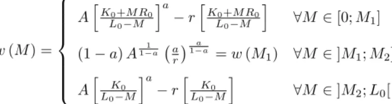
R (M ) = 8 > > > > > > < > > > > > > : R0= (s c)2+ 8M 2 [0; M1] R1(M ) = M1 h (L0 M ) aAr 1 1 a K 0 i 8M 2 ]M1; M2] R2= 0 8M 2 ]M2; L0[ (24) V (M ) = 8 > > > > > > < > > > > > > : V0= 1(1 + ) (1 + r) 1 1+ R 2+ 1+ 0 8M 2 [0; M1] V1(M ) = (1+r) 1 1+ [R1(M )] 1 1+ [(2 + ) R 0 R1(M )] 8M 2 ]M1; M2] V2= (1 + ) 2+s c 2+ 1+ 8M 2 ]M2; L0[ (25)
2.4
The developing country wage
For the time being, we assume that the number of migrants M is exogenous. Later on, we will show how the number of migrants is determined as an equilibrium value.
Labor is remunerated with the residual from the sell of the output and the cost of capital: wL = A (K)a(L)1 a rK8 . The equilibrium wage rate w is:
w (k) = A (k)a rk: (26)
The assumption according to which the marginal productivity of capital is higher than the interest rate without migration (equation 4) implies that the wage rate without migration is positive: k0< aAr 1 1 a =) k0< Ar 1 1 a () w0> 0.
According to equation (26), the wage rate depends on the capital intensity. Thus, there is a need to distinguish between three di¤erent cases.
1st case: M M1(no investment constraint)
Then, the remitted amount per migrant is R0, independent from M . The capital intensity
becomes:
k (M ) = K0+ M R0 L0 M
: (27)
8 Here, remittances do not have a negative impact on labour supply because they are invested and not sent
for altruistic reasons (Chami et al., 2005; Naiditch and Vranceanu, 2009), nor for an insurance motive (Azam et Gubert, 2005).
The wage rate in the developing country then is: w(M ) = A K0+ M R0 L0 M a r K0+ M R0 L0 M : (28)
with w(M = 0) = A (k0)a rk0= w0> 0 and limM!M1w(M ) = w (M1) = (1 a) A 1 1 a a r a 1 a: 2ndcase: M 1< M M2 (constrained investment)
Then, the remitted amount per migrant is R1(M ) such that: 8M; k (M) = k (M1) = aAr
1 1 a
: The wage rate in the developing country is:
w(M ) = w (M1) = (1 a) A 1 1 a a r a 1 a : (29) 3rd case: M 2< M < L0 (no investment)
Then, the remitted amount per migrant is null; the capital intensity becomes: 8M; k (M) =
K0 L0 M aA r 1 1 a:
The wage in the developing country is:
w(M ) = A K0 L0 M a r K0 L0 M : (30)
If we were to summarize the three cases, we can de…ne a function w representing the wage in the developing country depending on M :
w (M ) = 8 > > > > > > < > > > > > > : AhK0+M R0 L0 M ia rhK0+M R0 L0 M i 8M 2 [0; M1] (1 a) A11a a r a 1 a = w (M 1) 8M 2 ]M1; M2] Ah K0 L0 M ia rh K0 L0 M i 8M 2 ]M2; L0[ (31)
Proposition 1 The wage in the developing country is an increasing function of the number of migrants over [0; M1]. It is a constant function of the number of migrants over ]M1; M2]. There
is a discontinuity in M2; it increases and then decreases over ]M2; L0[. It reaches its maximum
over [M1; M2] and in M3 = L0 aAr
1 1 aK
0. It is null when the emigration level reaches the
threshold M4 L0 Ar
1 1 a
K0:
Proof. The proof can be found in Appendix A.2. Figure 1 depicts the wage as a function of M:
w(M1) M w(M) w0 M1 M2 M3 M4 R0>0 R1(M) R2=0
The wage rate in the developing country.
The wage rate in the developing country reaches its maximum over [M1; M2] and then again
in M3: w(M1) = w (M3) = (1 a) A 1 1 a a r a 1 a > w0> 0: (32)
We can notice that the maximum wage is independent from the remitted amount. It is reached for the …rst time in M1 which decreases with R0. Thus, the higher the optimal remitted amount
per migrant, the faster the maximum wage is reached. Yet, for any migration level below M1, the
net remitted amount increases with the net bene…t from migration and decreases with transaction costs. Thus, the higher the host country wage and the lower the migratory and transaction costs, the faster the maximum wage is reached.
2.5
The indirect utility of the resident
At the beginning of the period 0, the resident earns a wage w (M ). To keep the model simple, we assume that due to imperfections in the …nancial markets he cannot invest in productive activities (he can save money, but at a zero interest rate).
Then, if C0r is the resident’s consumption at the beginning of the period and C1r his …nal
consumption, his optimization program is: 8 > > > > > > < > > > > > > : max(C0r;C1r)U (C0r; C1r) s.t. C0r+ C1r= w (M ) and C0r> 0 , C1r> 0:
We assume that the resident and the migrant have the same utility function and the same prefer-ence for present consumption: U (C0r; C1r) = ln C0r+1+1 ln C1r.
The optimization program of the resident becomes: 8 > > < > > : maxC0r;C1r h ln C0r+1+1 ln (w (M ) C0r) i s.t. 0 < C0r< w (M ) :
The …rst order condition dU (C0r)=dC0r= 0 implies:
8 > > < > > : C0r= 1+2+ w(M ) > 0 C1r= 2+1 w(M ) > 0
For optimal consumption levels, the indirect utility of the resident is: U (C0r; C1r) = ln ( 1 + 2 + 1 2 + 1 1+ w(M )2+1+ ) (33) U (C0r; C1r) = ln (W (M )) , with W (M ) 1 + 2 + 1 2 + 1 1+ w(M )2+1+ : (34)
We previously showed that the wage in the developing country depends on the number of migrants. We can then de…ne the function W representing (the exponential of) the indirect utility of the resident: W (M ) = 8 > > > > > > < > > > > > > : W0(M ) 1+2+ 2+1 1 1+ n AhK0+M R0 L0 M ia rhK0+M R0 L0 M io2+ 1+ 8M 2 [0; M1] W1 1+2+ 2+1 1 1+ n (1 a) A11a a r a 1 ao 2+ 1+ 8M 2 ]M1; M2] W2(M ) 1+2+ 2+1 1 1+ n Ah K0 L0 M ia rh K0 L0 M io2+ 1+ 8M 2 ]M2; L0[ (35)
3
Migratory equilibria
3.1
The equilibrium number of migrants
In autarky all the citizens of the developing country work in their origin country and are paid the wage rate w0. When migration is allowed, individuals have to make a choice: they can either stay
in their origin country and be paid the wage rate w(M ), or migrate to the developed country. If they migrate, they get paid the wage rate s, need to pay a constant migratory cost c, and can remit a gross amount T of which a part R is invested in their origin country.
His decision to migrate thus depends on anticipated wages in both countries, on migratory and transaction costs and on the prospective return on his investment.
Our de…nition of equilibrium implies an implicit dynamics, with workers leaving one after the other (but, why not, at a very short interval). As all workers are identical in this model, who does migrate before the other ultimately depends on "the speed of packing luggage". At the migratory equilibrium, the marginal worker (i.e. the worker whose turn has come to take the decision) is indi¤erent between migrating to the developed country and staying in the origin country. In equilibrium, migrants’utility is identical to the stayers’utility.
Formally, the equilibrium condition is:
ln V (M ) = ln W (M ) : (36) Formally, it means: 8 > > > > > > < > > > > > > : V0= W0(M ) , M 2 [0; M1] V1(M ) = W1 , M 2 ]M1; M2] V2= W2(M ) , M 2 ]M2; L0[ (37)
Proposition 2 There are four types of equilibria:
When V2> W1, there is total migration (equilibrium 0).
When V2 W1< V0, there are one or two steady equilibria: one between M1 and M2 and
the other between M2 and M3 (only under certain conditions) (equilibrium 1).
When W0 < V0 W1, there is a single steady equilibrium before M1 (M ). Under certain
conditions, there exists another steady migratory equilibrium between M2 and M3
(equilib-rium 2).
When V0 W0, there is no migration (equilibrium 3).
Proof. The proof can be found in Appendix A.3.
W1 M W(M) W0 M1 M2 M3 M4 V0 V2
Eq. 0: total migration
W1 M W(M) W0 M1 M2 M3 M4 V0 V2
Eq. 1: two steady equilibria above M1
W1 M W(M) W0 M1 M2 M3 M4 V0 V2
Eq. 2: one steady equilibrium before M1
M W(M) W0 M1 M2 W1 M3 M4 V0 V2 Eq. 3: no migration Figure 2: Various Types of Equilibria
Thus, there may be total emigration at the equilibrium (equilibrium 0): when V2 > W (M1),
the developing country is deserted at the equilibrium. Galor’s result (1986) holds despite invested remittances. Formally, there is total migration when V2 > W (M1) () (s c) > w (M1). In
other words, there is total migration when the migratory cost is too low, whatever the level of transaction costs: V2> W (M1) () c < s (1 a) A 1 1 a a r a 1 a : (38)
There is a high steady equilibrium (between M1 and M2, equilibrium 1) when the migratory
cost (function of transaction costs) is low, but not too low:
1 a 1aa (1 a) A 1 1 a a r a 1 a
There is a steady migratory equilibrium below M1 (equilibrium 2) when the migratory cost
(function of transaction costs) is neither too low, nor too high:
W0< V0 W (M1) () s (1 a) A11a a r a 1 a [ (1 + r)]2+1 c < s (A (k0) a r (k0)) [ (1 + r)]2+1 : (40)
Finally, there is no migration at all (equilibrium 3) when the migratory cost (function of transaction costs) is too high:
V0 W0, c s
(A (k0)a r (k0))
[ (1 + r)]2+1
: (41)
For the sake of parsimony, we study hereafter only the Equilibrium 2. Indeed, this equilibrium is non total, that is not all the residents leave the developing country; this seems to be a general migration pattern. Furthermore, compared to con…guration 1 (two stable non-total equilibria), Equilibrium 2 is likely to occur for the broadest range of parameters.
3.2
Properties of the Equilibrium 2
Let M denote the equilibrium number of migrants. In this con…guration, the equilibrium number of migrants is below M1: M M1(with utilities ranked: ln W0< ln V0 ln W (M1)). We denote
by k the capital intensity when migration reaches M . Thus, any migrant’s utility is ln V0= ln 1 (1 + ) (1 + r)
1 1+ R
2+ 1+
0 , and any resident’s utility
is ln W0(M ) = ln " 1+ 2+ 1 2+ 1 1+ n AhK0+M R0 L0 M ia rhK0+M R0 L0 M io2+ 1+ # .
How does the equilibrium number of migrants vary with the gross and net remitted amounts? and with migratory and transaction costs?
We have shown (equation 9) that for M < M1; the optimal amount of remittances R0 = 1
2+ [ (s c) ] depends on (s c); and : Changes in these parameters (for instance an
increase in the host country wage s) induces changes in the remitted amount. In turn, changes in parameters that push up the remitted amount per migrant, also push up the migrant’s indirect utility V0.
On the other hand, for a constant number of migrants below M1, the wage in the origin country
(26), we know that:@w(M )@R 0 0 () h aA (k (M ))a 1 ri@k(M )@R 0 0 () k (M) aA r 1 1 a () M M1:
Thus, for a constant number of migrants below M1, both residents and migrants’ utilities
increase when changes in parameters push up the optimal remitted amount. The increase in the residents’ utility has a negative e¤ect on the equilibrium number of migrants, whereas the increase in the migrants’ utility has a positive e¤ect on the equilibrium number of migrants. In our framework, we can show that:
Proposition 3 The equilibrium number of migrants M and the optimal amount of remittances per migrant R0 are positively related.
Proof. The proof can be found in Appendix A.4.
When remittances per migrant increase, the induced increase in the migrant’s utility is higher than the induced increase in the resident’s utility. Note that M is an increasing function of the remitted amount whereas M1 is a decreasing function of remittances.
Proposition 4 The higher the net migratory bene…t (s c), the higher the equilibrium migration M , and the higher the remittances per migrant, R0.
The smaller the …xed transaction costs ( ), the higher the equilibrium migration M , and the higher the remittances per migrant R0.
If a 2+1 , the smaller the variable transaction costs (1 ) the higher the equilibrium migra-tion M , and the higher the remittances per migrant R0.
Proof. The proof of the …rst part of these sentences can be found in Appendix A.4. The second part, pertaining to the relationship between parameters and optimal remittances directly follow from equation (11).
In equilibrium, shocks to parameters move both remittances per migrant and the total number of migrants in the same direction. As a consequence, if this equilibrium prevails, one should observe a positive correlation between the amount of remittances per migrant and the equilibrium number of migrants.
W(M1) W(M) W0 M1 V0 V’0 M* M’* M’1 W(M1) W(M) W0 M1 V0 V’0 M* M’* M’1
Impact of an increase of the net migratory bene…t.
The initial equilibrium is obtained for V0 = W (M ); where the number of migrants is M :
A utility increasing shock (e.g. s increases) would lead to higher optimal remittances and more investment, thus shifting W (M ) upwards (the blue positive slope curve). All things equal, the number of migrant would decline. Yet, the increase in s (and in remittances that are invested) implies a higher utility for the migrants too, which goes to V00 (blue horizontal line). The new
equilibrium is obtained for M0 : The net migratory e¤ect is positive M0 > M ; (but smaller as compared to the situation where remittances cannot be invested, thus do not push up wages in the origin country).
In the next section, we aim at backing the theoretical model with some empirical evidence. Despite the substantial interest in this …eld, suitable data on remittances are so far very scarce; in particular, data on migratory costs and transaction costs are not available for a large group of countries; therefore, we could not test directly the relationships stated in Proposition 4. As a second best solution, we will analyze the equilibrium comovement between remittances per migrant and total number of migrants (Proposition 3).
4
The empirical analysis
4.1
The EECA region
Countries under scrutiny belong to the group of formerly centrally planned economies in Eastern Europe and Central Asia (EECA hereafter), and build on the World Bank’s o¢ cial delineation of
the zone. In 2006, there were 28 countries in this group.9 Three countries had to be removed from the analysis (Tajikistan, Turkmenistan and Uzbekistan), since we did not have any information on the amount of remittances they received. Thus, we will study at most 25 countries.
This group of countries provides for a worthy case study, since they have a similar economic history; most important for our analysis, new migration is driven essentially by economic motives. The region also provides enough diversity in terms of development levels, growth in population and new migration to allow for meaningful tests of our model.
EECA countries total 444 million people. In 2000, the average crude birth rate in EECA countries was 12.7 per thousand people and the crude death rate was around 11.7 per thousand; net emigration represented 2.5 million people; globally, in 2000, the EECA population grew by 0.12% (WDI …gures). More speci…cally, in 2000, most EECA countries saw their population decrease; in 4 countries, it grew by less than 1% (Slovenia, Montenegro, Macedonia, FYR, Azerbaijan); and in only 6 countries, the population growth rate was between 1% and 2.1% (Uzbekistan, Kyrgyztan, Tajikistan, Turkmenistan, Turkey, Bosnia and Herzegovina).
According to a recent study by the World Bank (2006), migration ‡ows in EECA tend to move in a largely bipolar pattern. Much of the emigration in Western EECA10 (42%) is directed toward Western Europe, while much emigration from the CIS11 remains within the CIS (80%). Germany is the most important destination country outside EECA for migrants from the region, while Israel was an important destination in the …rst half of the 1990s. Russia is the main intra-CIS destination. The United Kingdom is becoming a destination for migrants from the EECA countries of the European Union (EU). In 2000, according to the Global Migrant Origin Database, the largest stocks of migrants from EECA were located in Russia (11,553,062), Ukraine (6,669,273), Germany (3,883,761), Kazakhstan (2,838,336), the United States (2,177,586), Belarus (1,270,862),
9 The World Bank includes in its "Europe and Centra Asia" group of countries: Albania, Armenia, Azerbaijan,
Belarus, Bosnia and Herzegovina, Bulgaria, Croatia, Czech Republic, Estonia, the Former Yugoslav Republic of (FYR) Macedonia, Georgia, Hungary, Kazakhstan, Kyrgyztan, Latvia, Lithuania, Moldova, Poland, Romania, Russian Federation, Serbia and Montenegro, Slovak Republic, Slovenia, Tajikistan, Turkey, Turkmenistan, Ukraine, and Uzbekistan.
1 0 Western ECA: the EU-10 new member countries, plus Bosnia and Herzegovina, Serbia, Montenegro, Albania,
Croatia, and FYR Macedonia.
1 1CIS = Commonwealth of Independent States (Armenia, Azerbaijan, Belarus, Georgia, Kazakhstan, Kyrgyztan,
Israel (1,216,672) and Uzbekistan (1,034,601).
For many EECA countries, remittances are the second most important source of external …-nancing after foreign direct investment. They represented 0.87% of the region’s GDP in 1995, 1.45% in 2000 and 1.37% in 2005. But these …gures hide wide disparities. In 2000, for example, remittances represented more than 10% of the GDP of Moldova (30.8%), Tajikistan, Armenia, Bosnia and Herzegovina, Albania, and Kyrgyztan. It represented between 1% and 5% in several countries (Bulgaria, Georgia, Azerbaijan, Romania, Macedonia FYR, Croatia, Serbia and Mon-tenegro, Latvia, Poland, Lithuania and Estonia). Finally, it represented less than 1% only in the following countries (Belarus, Czech Republic, Slovenia, Ukraine, Russian Federation, Kazakhstan, Hungary, Turkey and Slovak Republic) (WDI …gures).
Generally remittance ‡ows in EECA follow the same two-bloc pattern as migration. The EU is the main source of remittances, accounting for three quarters of the total, and the resource-rich CIS are the other main source, accounting for 10%. The amount contributed by the EU-10 countries12 is also signi…cant (World Bank, 2006).
Results from surveys with returned migrants in EECA found that a non negligible share of remittances is invested in capital formation. The World Bank (2006) claims that if the majority of remittances are utilized for funding consumption of food and clothing, large quantities are also used for education and savings (over 10%); smaller amounts are spent on direct investment in business (less than 5%). For example, in Armenia, empirical evidence suggests that the propensity to save out of remittance income is high (almost 40%) and remarkably consistent across studies (Roberts et al., 2004). In Albania, a study conducted on the national level in 1998 suggests that 17% of the investments in small and medium size enterprises came from money accumulated while working abroad (Kule et al. 2002). Other sources claim that almost 30% of investments in Albanian small and middle sized enterprises were primarily …nanced by remittances from family members working abroad (INSTAT, 2003). Another survey conducted in the Korçë district in Albania in 2002 suggests that around 5% of receiving households use the money from remittances to invest
1 2 EU-10: the Czech Republic, Poland, Hungary, Slovakia, Slovenia, Latvia, Lithuania, Estonia, Bulgaria and
in non-farm business, and around 17% use remittances for agricultural investments (Arrehag et al., 2005). An IOM survey of Serbian households with relatives living in Switzerland conducted in two rural regions of Serbia in 2006 showed that approximately 1/4thof surveyed households have
used remittances to expand agricultural production and 8% to invest in a business (SECO, 2007). A World Bank survey (World Bank, 2006) shows that in Kyrgyztan, 11% of households receiving remittances report saving remittances. In Tajikistan, about 9% report saving remittances and 2.5% report investing in business. In Moldova, according to a study conducted in 2006, nearly 30% of recipient households save over US$500 (Orozco, 2007).
4.2
Data and de…nition of main variables
4.2.1 Migration data
Problems inherent to migration data
Compiling data on migration stocks and ‡ows is quite complicated for several reasons. Of-…cial data often underestimate migrants stocks and ‡ows because of di¢ culties that arise from di¤erences across countries in the de…nition of a migrant (foreign born versus foreign nationality), reporting lags in census data, and under-reporting of irregular migration. These problems arise, in part due to a lack of standardized de…nitions and common reporting standards (and inadequate adherence to these standards where they exist). The commonly accepted UN de…nition describes a “migrant” as a person living outside his or her country of birth.
Some problems are more speci…c to EECA countries. Indeed, the type, direction and mag-nitude of the ‡ows in the region have changed dramatically since the beginning of economic transition, liberalization of societies and retrieved human rights (including the cross-border free-dom of movement), and the emergence of 22 new states. The extent to which the successor states have implemented statistic systems able to properly measure total migration ‡ows and disaggre-gate these ‡ows by nationality varies considerably. Moreover, the break-up of the Soviet Union, Yugoslavia, and Czechoslovakia created a large number of “statistical migrants”.13
1 3Statistical migrants refers to persons who migrated internally while those countries existed, thus not qualifying
as a migrant under the UN de…nition at the time, but who began to be counted as migrants when those countries broke apart even though they did not move again (World Bank, 2006).
Databases
For the purpose of this paper, we need an estimate of the total stock of emigrants from each EECA countries. To our knowledge, the only databases providing that information are the Global Migrant Origin Database (Migration DRC, University of Sussex) and the database prepared by the Development Prospects Group (World Bank).
We get the University of Sussex data from the Development Research Centre on Migration, Globalisation and Poverty (Migration DRC), an independent organization for the study of migra-tions.14 The data are generated by disaggregating the information on migrant stocks in each destination country or economy as given in its census to get a 226x226 matrix of origin-destination stocks by country. In essence, the Migration DRC database extends the basic stock data on in-ternational migration published by the United Nations.15 Four versions of the database are
currently available and we choose to use the latest version of the database, given that its authors strived to correct for some biases speci…c to all stock data inferred from census data.16 The
reference period is the 2000 round of population censuses. In order to get estimates of the total stock of migrants from each EECA country in 2000, we summed the stocks of migrants from the same origin country in all destination countries. This variable is denoted by M IGRS.
The database prepared by the Development Prospects Group of the World Bank is a variant of the Migration DRC database. The latter was updated using the most recent census data and unidenti…ed migrants were allocated only to two broad categories, “other South” and “other North” (Ratha and Shaw, 2007). We used this database to get other estimates of the stocks of migrants from each EECA country in 2000. This variable is denoted by M IGRW B.
4.2.2 Two kinds of remittances data
The main sources of o¢ cial data on migrants’remittances are the annual balance of payments of various countries, which are compiled in the Balance of Payments Yearbook published annually
1 4 See: www.migrationdrc.org/index.html
1 5 See http://www.un.org/esa/population/ publications/migstock/2003TrendsMigstock.pdf
1 6 The Migration DRC methodology is available online at: www.migrationdrc.org/ research/
by the International Monetary Fund (IMF). The IMF data include two categories of data: work-ers’ remittances including current transfers by migrants who are employed or intend to remain employed for more than a year in another economy in which they are considered residents, and workers’ remittances and compensation of employees made up of current transfers by migrant workers and wages and salaries earned by nonresident workers.
While the categories used by the IMF are well de…ned, there are several problems associated with their worldwide implementation that can a¤ect their comparability. On the one hand, o¢ cial remittance …gures may underestimate the size of ‡ows because they fail to capture informal remit-tance transfers, including sending cash back with returning migrants or by carrying cash and/or goods when migrants return home. Only two countries in EECA –Moldova and Russia –attempt to capture remittances sent through informal channels in the balance of payments statistics (World Bank, 2006). On the other hand, o¢ cial remittance …gures may also overestimate the size of the ‡ows. Other types of monetary transfers –including illicit ones –cannot always be distinguished from remittances (Bilsborrow et al., 1997).
For the purpose of this study, we constructed two di¤erent variables from the WDI database: received workers’remittances and compensation of employees (US$) and receipts of workers’remit-tances (US$). In 2000, the …rst one, denoted by REM CE, was available for 25 EECA countries, while the second, denoted REM , was only available for 18 countries.17 In order to be able to
compare these …gures in the di¤erent countries, we …rst converted them into local currency units (LCU) using the o¢ cial exchange rate of the WDI database and then used a PPP conversion factor.18 The WDI database o¤ers two di¤erent PPP conversion factors: one for GDP and
one for private consumption (i.e., household …nal consumption expenditure). Thus, we built four variables representing remittances in PPP: REM CEP P P 1 and REM P P 1 (using the PPP con-version factor for GDP), and REM CEP P P 2 and REM P P P 2 (using the PPP concon-version factor for private consumption).
1 7 Data were missing for Belarus, Bulgaria, Czech Republic, Russian Federation, Serbia and Montenegro, Slovak
Republic and Ukraine.
1 8 A PPP conversion factor is the number of units of a country’s currency required to buy the same amounts of
4.2.3 Two assumptions about the investment rate of remittances
In this paper, we want to estimate the link between invested remittances and the number of equilibrium migrants. However, there is no information on the rate of investment of remittances sent by migrants. Thus, we made two di¤erent assumptions about the proportion of invested remittances.
According to the …rst hypothesis, invested remittances contribute to gross …xed capital for-mation (GFCF); the proportion of invested remittances out of total remittances is similar to the proportion of GFCF out of GDP. Thus, we build a …rst couple of variables, denoted by REM CEP P P iGF CF and REM P P P iGF CF (with i = 1, 2), representing invested remittances in 2000 as the product of remittances and the share of GFCF in GDP, for each EECA country in the database (the cross-country average rate was of 21% in 2000).
According to the second hypothesis, we assume that migrants act in the same way as foreign investors; the proportion of invested remittances out of total remittances is then similar to the proportion of foreign direct investment (FDI) out of GDP. Thus, we build a second couple of variables, denoted by REM P P P iCEF DI and REM P P P iF DI (i = 1, 2), representing invested remittances in 2000 as the product of remittances and the ratio of net in‡ows of FDI to GDP, for each EECA country in the database (the cross-country average rate was of 4.5% in 2000).
All the data come from the World Development Indicators (WDI) database. 4.2.4 Control variables
In our econometric model, we include as control variables either the GDP per capita (PPP) or the wage rate (PPP).
In the …rst case, we take GDP per capita as a proxy for the economic incentives to leave one’s origin country. Indeed, neoclassical economics stipulates that migration can be explained by the di¤erential between anticipated wages in the origin and the potential host countries. But since we do not have information on bilateral remittances, we only use the level of GDP per capita in origin countries as a push factor potentially explaining migration. These data are taken from the WDI database and denoted by GDP cap.
By the same token, in the second case, we use the wage rate in the origin country as a control variable. Wage rates data come from the International Labor Organization (ILO) where they can be found in LCU. Then, we built two variables representing wage rates in PPP: W AGEP P P 1 (using the PPP conversion factor for GDP) and W AGEP P P 2 (using the PPP conversion factor for private consumption).
4.2.5 Descriptive statistics
Descriptive statistics for the sample are shown in the following table:
Variable N Mean Standard Deviation Minimum Maximum MIGRS 25 1,665,179.80 2,531,169.06 108,897.00 12,098,614.00 MIGRWB 25 1,780,151.42 2,482,629.83 133,964.91 11,480,137.37 REMCEPPP1 23 1,344,052,665 2,289,061,735 635,0576.49 8,869,947,794 REMCEPPP2 24 1,735,799,593 2,733,693,389 7,138,959.92 10,068,748,556 REMPPP1 16 963,223,143 2,265,985,617 722,652.57 8,869,947,794 REMPPP2 17 1,219,871,966 2,527,829,801 812,365.26 10,068,748,556 GFCF (% of GDP) 25 21.07 4.16 12.28 27.98 FDI (% of GDP) 24 4.47 2.91 0.28 9.90 REMCEPPP1GFCF 23 260,010,275 425,880,953 165,0467.58 1,808,851,637 REMCEPPP2GFCF 24 336,527,855 503,452,378 1,855,362.56 2,053,323,507 REMCEPPP1FDI 22 30,103,229.28 43,188,550.82 437,394.20 197,073,664 REMCEPPP2FDI 23 39,457,716.17 52,016,291.14 491,693.89 221,917,180 REMPPP1GFCF 16 208,069,910 470,478,818 187,812.02 1,808,851,637 REMPPP2GFCF 17 262,914,875 525,338,320 211,127.69 2,053,323,507 REMPPP1FDI 15 24,333,155.63 45,727,815.89 49,772.50 175,151,217 REMPPP2FDI 16 31,841,504.10 51,905,057.04 55,951.43 197,231,144
As can be seen, the two assumptions made about the rate of investment of remittances can be considered as a high hypothesis (when the rate of investment of remittances is proxied by the proportion of GFCF in GDP) and a low hypothesis (when the rate of investment of remittances is proxied by the proportion of FDI in GDP).
4.3
Empirical estimates
4.3.1 The model
We want to analyze the equilibrium co-movements between invested remittances per migrant and the number of migrants. Proposition 3 claims that the two variables are positively correlated.
Thus, we postulate that the equilibrium number of migrants, M , (we can drop the star in this section), can be written as a function of invested remittances per migrants at the equilibrium, IRM, a control variable, control, and an error term, u:
Taking the log, we get: ln(M ) = b0+ b1ln (IR) + b2ln(control) + "; (43) with b0= ln(1+0) 1; b1= 1 1+ 1; b2= 2 1+ 1; " = ln(u) 1+ 1:
All the coe¢ cients of equation (42) can then be expressed as a function of the coe¢ cients of
equation (43): 8 > > > > > > < > > > > > > : b0=ln(1+0) 1 b1=1+11 b2=1+21 () 8 > > > > > > < > > > > > > : 0= exp 1 bb01 1= 1 bb11 2= 1 bb21 (44)
Thus, if we can estimate equation (43) and get estimates of b0, b1 and b2, denoted by ^b0, ^b1 and
^b2, we can infer estimates of
0, 1 and 2, denoted by ^0, ^1 and ^2.
If our Proposition 3 is correct, the equilibrium number of migrants is positively related to the remitted amount per migrant. Thus, we expect ^1to be statistically greater than 0, which is true if ^b1is statistically greater than 0 and smaller than 1. In addition, we expect the control variables,
either GDP per capita or the wage in the origin country, to have a negative impact on the number of migrants; thus we expect ^2 to be statistically negative.
4.3.2 Methodology and Results
In equation (43) the dependent variable is the number of migrants. As previously explained, the number of migrants can be taken either from the Global Migrant Origin Database or from the database prepared by the Development Prospects Group of the World Bank. Likewise, the main independent variable, invested remittances, can be measured either by workers’remittances and compensation of employees or by workers’ remittances only, multiplied either by the gross …xed capital formation expressed as a percentage of GDP or by net in‡ows of foreign direct investment expressed as a percentage of GDP. Finally, the control variable can be either GDP per capita, or the wage rate measured with the PPP conversion factor either for GDP or for private consumption.
Hence, in a general form, the basic equation is: ln 8 > > < > > : M IGRW B M IGRS 9 > > = > > ; = b0+ b1ln 8 > > > > > > > > > > < > > > > > > > > > > :
REM CEP P P iGF CF REM CEP P P iF DI REM P P P iGF CF REM P P P iF DI 9 > > > > > > > > > > = > > > > > > > > > > ; + b2ln 8 > > > > > > < > > > > > > : GDP cap W AGEP P P 1 W AGEP P P 2 9 > > > > > > = > > > > > > ; + ": (45) OLS estimates
In a …rst step, we use OLS to estimate various variants of this equation. The results of the regressions using the World Bank database for the stocks of migrants (M IGRW B) are as follows:19
Variables (1) (2) (3) (4) Intercept 12.34*** (4.23) 15.09*** (3.77) 13.16*** (5.43) 13.54*** (4.18) LREMCEPPP2GFCF 0.39*** (3.62) LREMCEPPP2FDI 0.31** (2.14) LREMPPP2GFCF 0.25*** (3.81) LREMPPP2FDI 0.24***(3.19) LGDPcap -0.65** (-2.33) -0.72* (-2.04) -0.44* (-1.80) -0.42 (-1.35) N 24 23 17 16 R² 0.44 0.31 0.56 0.53 adj. R² 0.39 0.24 0.50 0.46 Shapiro-Wilk test (p-value in brackets) 0.92825 (0.0891) 0.905946 (0.0336) 0.913336 (0.1139) 0.884403 (0.0455) F value (b1 = 1) (p-value in brackets) 33.14 (<.0001) 23.19 (0.0001) 131.42 (<.0001) 97.57 (<.0001) t-student in brackets; *** significant to 1%; ** significant to 5%; * significant to 10%
Variables (5) (6) (7) (8) Intercept 11.08*** (4.46) 13.38*** (4.68) 12.08*** (6.87) 12.53*** (6.94) LREMCEPPP1GFCF 0.40*** (3.21) LREMCEPPP1FDI 0.634** (2.27) LREMPPP1GFCF 0.27*** (3.21) LREMPPP1FDI 0.26*** (3.49) LWAGEppp1 -0.76*** (-3.02) -0.85*** (-2.92) -0.50** (-2.27) -0.49* (-2.13) N 20 19 13 12 R² 0.50 0.44 0.58 0.66 adj. R² 0.44 0.37 0.50 0.58 Shapiro-Wilk test (p-value in brackets) 0.965432 (0.6570) 0.946293 (0.3143) 0.877033 (0.0650) 0.863554 (0.0542) F value (b1 = 1) (p-value in brackets) 23.78 (0.0001) 19.85 (0.0004) 76.98 (<.0001) 93.73 (<.0001) t-student in brackets; *** significant to 1%; ** significant to 5%; * significant to 10%
Variables (9) (10) (11) (12) Intercept 10.83*** (4.52) 12.83*** (4.63) 11.69*** (7.07) 12.00*** (6.98) LREMCEPPP2GFCF 0.40*** (3.48) LREMCEPPP2FDI 0.36** (2.55) LREMPPP2GFCF 0.27*** (3.63) LREMPPP2FDI 0.27*** (3.99) LWAGEppp2 -0.73** (-2.87) -0.80** (-2.71) -0.45* (-2.06) -0.42* (-1.89) N 21 20 14 13 R² 0.48 0.42 0.58 0.65 adj. R² 0.43 0.35 0.50 0.58 Shapiro-Wilk test (p-value in brackets) 0.964065 (0.6015) 0.963052 (0.6065) 0.882883 (0.0639) 0.854326 (0.0325) F value (b1 = 1) 26,52 31 21.03 13.19 110.05
In 9 models out of 12 the coe¢ cient ^b1 is statistically positive and smaller than 1 at the 99%
con…dence level; it is always statistically positive and smaller than 1 at the 95% con…dence level. The results corroborate Proposition 3. Furthermore, the estimates of ^b1 2 [0:24; 0:63]. This is
tantamount to an elasticity of the equilibrium number of migrants with respect to remittances per migrant equal to 1= b1
1 b1 2 [0:31; 1:7].
Concerning the coe¢ cient ^b2, it is negative as expected and statistically signi…cant in 6 models
out of 12 at the 95% con…dence level, and in all models but one at the 90% con…dence level.
Bootstrap estimations
In the previous regressions, the sample size varies from 12 to 24. This small sample size may raise di¢ culties determining con…dence intervals of coe¢ cients, since these intervals depend on assumptions on the distribution of the error term of the regression model. If these assumptions are no longer satis…ed, standard con…dence intervals can no longer be de…ned. We did test the normality assumption of the residuals in the di¤erent models using a Shapiro-Wilk test:20 in 5
models, the p-value is higher than 0.1, so we cannot reject the null hypothesis that the residuals are normally distributed; however, when the p-value is between 0.05 and 0.1 (in 4 models), we reject the null hypothesis at the 90% con…dence level, and when it is between 0.01 and 0.05 (in 3 models), we reject the null hypothesis at the 95% con…dence level. Thus, in some cases, the con…dence intervals of these OLS coe¢ cients may be wrong.
In order to improve the robustness of our estimations, we resort to the bootstrap method proposed by Efron (1979), which allows the approximation of an unknown distribution by an empirical distribution obtained by a resampling process. Bootstrap is a resampling technique based on random sorts with replacement in the data forming a sample. The application of bootstrap methods to regression models helps approximate the distribution of the coe¢ cients (Freedman, 1981) and the distribution of the prediction errors when the regressors are data (Stine, 1985). Used to approximate the unknown distribution of a statistic by its empirical distribution, bootstrap methods are employed to improve the accuracy of statistical estimations (Juan and Lantz, 2001).
Following Juan and Lantz (2001), we used a percentile-t bootstrap procedure, resampling the residuals. At the 95% con…dence level, with 1000 resamples, we get the following results:
Model Variable Observed
Statistics Approximate Lower Confidence Limit Approximate Upper Confidence Limit 1 LREMCEPPP2GFCF 0.38637 0.25406 0.76687 LGDPCAP -0.64704 -3.27976 -0.33270 2 LREMCEPPP2FDI* 0.30716 0.14525 1.88117 LGDPCAP -0.72228 -3.75634 2.36405 3 LREMPPP2GFCF 0.24953 0.1510 0.62367 LGDPCAP -0.44352 -3.35808 2.64043 4 LREMPPP2FDI 0.24394 0.13043 0.86527 LGDPCAP -0.42301 -5.46452 4.62736
*: 90% confidence level interval: [0.16619; 0.96771]
Model Variable Observed
Statistics Approximate Lower Confidence Limit Approximate Upper Confidence Limit 5 LREMCEppp1GFCF* 0.39702 0.23385 1.04430 LWAGEppp1 -0.75881 -2.51281 -0.42981 6 LREMCEppp1FDI** 0.33753 -0.31596 1.80207 LWAGEppp1 -0.85292 -4.02815 -0.47920 7 LREMppp1GFCF 0.26765 0.04549 0.99177 LWAGEppp1 -0.50190 -4.11571 3.59820 8 LREMppp1FDI*** 0.26519 -0.37139 0.94213 LWAGEppp1 -0.49269 -4.47034 2.48687 *: 90% confidence level interval: [0.24854; 0.82102]
**: 90% confidence level interval: [0.17418; 1.17804] ***: 90% confidence level interval: [0.07674; 0.63844]
Model Variable Observed
Statistics Approximate Lower Confidence Limit Approximate Upper Confidence Limit 9 LREMCEPPP2GFCF 0.40297 0.25158 0.97288 LWAGEppp2 -0.72607 -2.59453 -0.40870 10 LREMCEPPP2FDI 0.35721 0.18936 1.44802 LWAGEppp2 -0.80129 -4.01409 -0.43552 11 LREMPPP2GFCF 0.27296 0.13848 0.94592 LWAGEppp2 -0.44606 -3.60403 2.40149 12 LREMPPP2FDI 0.27544 0.04540 0.84588 LWAGEppp2 -0.42412 -3.18863 2.34093
As can be seen, the average coe¢ cient (observed statistics) for both ^b1and ^b2are very much in
line with OLS estimations. Most important, according to the bootstrap results, ^b1is statistically
positive and smaller than 1 (as claimed in Proposition 3) in 7 models out of 12 at the 95% con…dence interval and in 10 models out of 12 at the 90% con…dence interval. So this more rigorous method for determining con…dence intervals does corroborate the OLS estimates.
4.3.3 Discussion
We tried to introduce other control variables to take into account institutional di¤erences between EECA countries. However, a dummy variable di¤erentiating East Europe countries from Central Asia countries is highly correlated with the GDP per capita (PPP) and the wage rate (PPP). Thus, it could not be introduced in the model. We also tried to take into account a possible lagged e¤ect of invested remittances and used variables on the received amount of remittances one year earlier (in 1999). The results are quite similar to those presented and corroborate our proposition.21 Finally, we tried to introduce a "pull factor" variable representing the attractiveness of foreign countries for potential migrants, but important data were missing.
We acknowledge the fact that our empirical estimations should be subject to caution due to the modest quality of the data. In particular, data on migration and remittances do not take into account illegal migrants nor informal remittances. But since informal remittances are rarely invested and illegal migrants seldom use formal channel to remit, this measurement problem in the data may not be as serious as it seems. A more rigorous analysis would build on a more precise measure of the investment rate of remittances. Unfortunately, such data are not yet available.
5
Social optimum
In this paper, we analyze the optimality of migratory policies from the point of view of the devel-oping country.22 A public planner may want to use policy levers to ensure that the equilibrium
number of migrants is optimal according to a social welfare criterion. Indeed, the policymaker has an impact on both the migratory cost (by rede…ning the migratory policy or by helping potential migrants cover migratory costs) and the international transaction cost (by redesigning regulations and standards imposed to money transfer operators, by improving controls over informal money transfer channels or by improving competition in this sector).
2 1 Using received remittances in 1999 as the main dependant variable, we …nd that in 7 models out of 12, the
OLS estimate of b1 is statistically positive and smaller than 1 at the 99% con…dence level; it is always statistically
positive and smaller than 1 at the 95% con…dence level. According to the bootstrap results, ^b1 is statistically
positive and smaller than 1 in 9 models out of 12 at the 95% con…dence interval and in all the models at the 90% con…dence interval.
2 2 In this model, migration has no impact on the host country. Thus, we cannot de…ne an optimal migratory