HAL Id: cea-01430168
https://hal-cea.archives-ouvertes.fr/cea-01430168
Submitted on 9 Jan 2017
HAL is a multi-disciplinary open access
archive for the deposit and dissemination of
sci-entific research documents, whether they are
pub-lished or not. The documents may come from
teaching and research institutions in France or
abroad, or from public or private research centers.
L’archive ouverte pluridisciplinaire HAL, est
destinée au dépôt et à la diffusion de documents
scientifiques de niveau recherche, publiés ou non,
émanant des établissements d’enseignement et de
recherche français ou étrangers, des laboratoires
publics ou privés.
Dust attenuation in z
1 galaxies from Herschel and
3D-HST Hα measurements
A. Puglisi, G. Rodighiero, A. Franceschini, M. Talia, Alessandro Cimatti, I.
Baronchelli, Emanuele Daddi, A. Renzini, K. Schawinski, C. Mancini, et al.
To cite this version:
A. Puglisi, G. Rodighiero, A. Franceschini, M. Talia, Alessandro Cimatti, et al.. Dust attenuation in
z
1 galaxies from Herschel and 3D-HST Hα measurements. Astronomy and Astrophysics - A&A,
EDP Sciences, 2016, 586, pp.A83. �10.1051/0004-6361/201526782�. �cea-01430168�
DOI:10.1051/0004-6361/201526782
c
ESO 2016
Astrophysics
&
Dust attenuation in z
∼
1 galaxies from Herschel and 3D-HST
H
α
measurements
A. Puglisi
1, G. Rodighiero
1, A. Franceschini
1, M. Talia
2,3, A. Cimatti
2, I. Baronchelli
1, E. Daddi
8, A. Renzini
4,
K. Schawinski
5, C. Mancini
1,4, J. Silverman
10, C. Gruppioni
3, D. Lutz
6, S. Berta
7, and S. J. Oliver
91 Dipartimento di Fisica e Astronomia, Università di Padova, vicolo dell’Osservatorio 2, 35122 Padova, Italy
e-mail: annagrazia.puglisi@studenti.unipd.it
2 Dipartimento di Fisica e Astronomia, Università di Bologna, via Ranzani 1, 40127 Bologna, Italy 3 INAF–Osservatorio Astronomico di Bologna, via Ranzani 1, 40127 Bologna, Italy
4 INAF–Osservatorio Astronomico di Padova, Vicolo dell’Osservatorio, 5, 35122 Padova, Italy
5 Institute for Astronomy, Departement of Physics, ETH Zurich, Wolfgang-Pauli-Strasse 27, 8093 Zurich, Switzerland 6 Max-Planck-Institut für extraterrestrische Physik, Giessenbachstrasse, 85748 Garching, Germany
7 Max-Planck-Institut für Extraterrestrische Physik (MPE), Postfach 1312, 85741 Garching, Germany
8 Laboratoire AIM-Paris-Saclay, CEA/DSM-CNRS-Université Paris Diderot, Irfu/Service d’Astrophysique, CEA Saclay,
Orme des Merisiers, 91191 Gif sur Yvette, France
9 Astronomy Centre, Dept. of Physics & Astronomy, University of Sussex, Brighton BN1 9QH, UK
10 Kavli Institute for the Physics and Mathematics of the Universe, Todai Institute for Advanced Study, the University of Tokyo,
277-8583 Kashiwa, Japan
Received 19 June 2015/ Accepted 28 November 2015
ABSTRACT
We combined the spectroscopic information from the 3D-HST survey with Herschel data to characterize the Hα dust attenuation properties of a sample of 79 main sequence star-forming galaxies at z ∼ 1 in the GOODS-S field. The sample was selected in the far-IR at λ= 100 and/or 160 µm and only includes galaxies with a secure Hα detection (S/N > 3). From the low resolution 3D-HST spectra we measured the redshifts and the Hα fluxes for the whole sample. (A factor of 1/1.2 was applied to the observed fluxes to remove the [NII] contamination.) The stellar masses (M?), infrared (LIR), and UV luminosities (LUV) were derived from the spectral energy
distributions by fitting multiband data from GALEX near-UV to SPIRE 500 µm. We estimated the continuum extinction Estar(B − V)
from both the IRX= LIR/LUVratio and the UV-slope, β, and found excellent agreement between the two. The nebular extinction was
estimated from comparison of the observed SFRHαand SFRUV. We obtained f = Estar(B − V)/Eneb(B − V)= 0.93 ± 0.06, which is
higher than the canonical value of f= 0.44 measured in the local Universe. Our derived dust correction produces good agreement between the Hα and IR+UV SFRs for galaxies with SFR >∼ 20 M /yr and M? >∼ 5 × 10¹⁰M , while objects with lower SFR and
M?seem to require a smaller f -factor (i.e. higher Hα extinction correction). Our results then imply that the nebular extinction for our
sample is comparable to extinction in the optical-UV continuum and suggest that the f -factor is a function of both M?and SFR, in
agreement with previous studies.
Key words.galaxies: star formation – galaxies: high-redshift – dust, extinction – infrared: ISM
1. Introduction
The rate at which a galaxy converts gas into stars, the star forma-tion rate (SFR), is a fundamental quantity for characterizing the evolutionary stage of the galaxy. The SFR can be measured in several ways, such as from the UV luminosity, the far-IR emis-sion, the recombination lines or the radio-continuum (Kennicutt 1998; Madau & Dickinson 2014), although each of these SFR tracers suffers from some uncertainties. Concerning the UV and optical indicators, the main source of uncertainty in the estimate of the SFR is the dust extinction, which strongly absorbs the flux emitted by stars at UV and optical wavelengths and re-emits it in the far-IR. As a result, an accurate quantification of the impact of dust on the galaxy’s integrated emission is crucial for precisely evaluating the SFR.
The dust distribution inside a galaxy can be described by a two-component model (Charlot & Fall 2000, e.g.), includ-ing a diffuse, optically thin component (the interstellar medium, ISM) and an optically-thick one (the birth cloud) related to the star-forming regions. The birth clouds have a finite lifetime
(τBC ∼ 107 yr) and consist of an inner HII region ionized by
young stars and bounded by an outer HI region. This model as-sumes that the stars are embedded in their birth clouds for some time and then disrupt them or migrate away into the ambient ISM of the galaxy. In this model the emission lines are only pro-duced in the HII regions of the birth clouds since the lifetime of the birth clouds is in general longer than the lifetimes of the stars producing most of the ionizing photons (∼3 × 10⁶yr). The emis-sion lines and the non-ionizing continuum from young stars are attenuated in the same way by dust in the outer HI envelopes of the birth clouds and the ambient ISM, but since the birth clouds have a finite lifetime, the non-ionizing continuum radiation from stars that live longer than the birth clouds is only attenuated by the ambient ISM (Charlot & Fall 2000). This two-component model was conceived to explain the higher extinction observed on the nebular lines with respect to the UV/optical stellar contin-uum in the local Universe (e.g., Fanelli et al. 1988;Mas-Hesse & Kunth 1999;Mayya et al. 2004;Cid Fernandes et al. 2005; Calzetti et al. 1994,2000). The relation between the color excess of the nebular regions and that of the stellar continuum derived Article published by EDP Sciences
byCalzetti et al.(1994,2000), i.e. f= Estar(B − V)/Eneb(B − V)=
0.44, has proven to be successful for local star-forming galaxies, while it is still unclear whether it holds true in the high redshift Universe.
The most secure method to quantify the amount of dust ex-tinction in the HII regions is by directly measuring the Balmer decrement (i.e., the Hα/Hβ line ratio). Nevertheless, such mea-surements are very challenging at z >∼ 0.5 since the Hα line is shifted to the less-accessible near-infrared window so indirect methods are often needed to infer the attenuation related to the nebular lines. Current studies of dust properties in high redshift galaxies lead to contrasting results. In fact, while some authors claim that the extinction related to the emission lines and to the stellar continuum are comparable in z ∼ 2 galaxies (e.g., Erb et al. 2006; Reddy et al. 2010, using UV-selection), other au-thors confirm the validity of the Calzetti et al. local relation (e.g., Förster Schreiber et al. 2009;Whitaker et al. 2014;Yoshikawa et al. 2010, for samples of mainly optical and/or near-IR selected sources). Some recent works have also suggested that the factor f = Estar(B − V)/Eneb(B − V) required to reconcile the various
SFR measurements is higher than those computed in the local Universe (e.g., Kashino et al. 2013; Pannella et al. 2015, on sBzk selections). These contrasting results found in the literature are not surprising, given the different and indirect methods used and/or the small and sometimes biased samples of most of these studies. Direct measurements of the Balmer decrement would be required on statistical samples of sources at high redshift to clarify dust properties of distant star-forming galaxies.
In the present paper we used near-infrared spectroscopic data from the 3D-HST survey (Brammer et al. 2012) and multiwave-length photometry to derive the differential attenuation on a sam-ple of 79 star-forming galaxies at z between 0.7 and 1.5, selected in the far-IR within the GOODS-South field. The presence of the far-IR photometry for the whole sample is very important, as these data allow us to robustly constrain the integrated dust emission. This kind of approach has been often applied to galax-ies in the local Universe (see, for example,Domínguez Sánchez et al. 2014), but only very occasionally at higher redshifts.
The paper is organized as follows. In Sect.2the properties of the sample and the data set are described. Section3presents the spectral analysis. Section 4 illustrates the computation of the physical quantities for the galaxies in the sample. Section5 describes the measurement of dust extinction on the Hα emis-sion. Section 6 presents a critical discussion about the results with careful attention to the assumption behind our analysis, and Sect.7summarizes the results.
Throughout this work, we adopt a standard cosmology (H0=
70 km s−1Mpc−1, Ω
m= 0.3, ΩΛ= 0.7) and assume aSalpeter
(1955) IMF.
2. Sample and data set
Our sample is selected in the far-IR using the Herschel obser-vations from the PACS Evolutionary Probe survey (PEP, Lutz et al. 2011) in the GOODS-South field, which has the deep-est sampling with PACS-Herschel photometry. The far-IR data are key to the purpose of this work because they allow us to strongly constrain the thermal emission by dust and therefore to infer robust estimates of the continuum dust attenuation for all the galaxies in the sample. The Herschel selected sample has been matched with objects at 0.7 < z < 1.5 from the 3D-HST survey catalog (Brammer et al. 2012;Skelton et al. 2014) for which the Hα line is observable with the G141 grism. For the
cross-correlation procedure we took advantage of the GOODS-Multiwavelength Southern Infrared Catalog (GOODS-MUSIC, Grazian et al. 2006), which collects the available photometry from ∼0.3 to 8 µm for the objects detected in the GOODS-S field. In the following we briefly describe the catalogs used and the sample selection procedure.
2.1. The Herschel/PEP survey
The PEP survey is a deep extragalactic survey based on the ob-servations of the PACS instrument at 70, 100, and 160 µm. The GOODS-South field is the deepest field analyzed by the PEP sur-vey, and it is the only one observed also at 70 µm. The 3σ limit in the GOODS-S field is 1.0 mJy, 1.2 mJy, and 2.4 mJy at 70, 100, and 160 µm, respectively.
PACS photometry was performed with a PSF fitting tool by adopting the positions of Spitzer MIPS 24 µm detected sources as priors. This approach was applied to maximize the depth of the extracted catalogs, to improve the deblending at longer wave-lengths and to optimize the band-merging of the Herschel pho-tometry to the available ancillary data in the UV-to-near-IR. As described inBerta et al.(2011,2013), the 24 µm were used as a bridge to match Herschel to Spitzer/IRAC (3.6 to 8.0 µm) and then to the optical bands. PACS prior source extraction followed the method described byMagnelli et al.(2009). The complete-ness of the catalogs was estimated through extensive Monte-Carlo simulations, and it turns to be on the order of 80% with flux limits of 1.39, 1.22, and 3.63 mJy at 70, 100, and 160 µm, respectively (see PEP full public data release1). We defer toLutz
et al.(2011) for further information on the PACS source extrac-tion performances.
2.2. Multiwavelength photometry 2.2.1. The GOODS-MUSIC catalog
The GOODS-MUSIC catalog reports photometric data for the sources detected in z and Ks bands in the GOODS-South area, and it is entirely based on public data. The catalog was pro-duced with an accurate PSF matching for space- and ground-based images of different resolutions and depths, and it includes 14847 objects. The photometric catalog was cross-correlated with a master catalog2released by the ESO-GOODS team that
summarizes all the information about the spectroscopic red-shifts collected from several surveys in the GOODS area. For the sources lacking a spectroscopic measurement,Grazian et al. (2006) computed a photometric redshift using a standard χ2
technique with a set of synthetic templates drawn from the PEGASE2.0 synthesis model (Fioc & Rocca-Volmerange 1997). The MUSIC catalog was extended bySantini et al.(2009) with the inclusion of the mid-infrared fluxes, obtained from MIPS ob-servations at 24 µm. This catalog was also used for computing the spectral energy distributions (SED, see Sect.4.1for more details about the SED-fitting).
2.2.2. GALEX, IRS-Spitzer and SPIRE observations
To increase the spectral coverage of the final sample, we added to the MUSIC photometry the GALEX near-UV observations at λ = 2310 Å acquired from the online catalog Mikulski Archive
1 http://www.mpe.mpg.de/ir/Research/PEP/DR1 2 www.eso.org/science/goods/spectroscopy/CDFS_
for Space Telescopes (MAST), the IRS observations at 16 µm (Teplitz et al. 2005), and the SPIRE data at 250, 350 and 500 µm (Oliver et al. 2012;Roseboom et al. 2010;Levenson et al. 2010; see alsoViero et al. 2013andGruppioni et al. 2013). Both the GALEX and the SPIRE observations are extremely important for the goal of this work. The GALEX data allow us to constrain the SED at UV wavelengths better, enabling a more accurate es-timate of the UV spectral slope β (see Sect.5.2and AppendixA for details). On the other hand, the SPIRE data improve the spec-tral coverage in the far-IR, thus allowing us to derive a robust estimate of the bolometric infrared luminosity (see Sect.4.1).
The SPIRE catalog is also selected with positional priors at 24 µm. SPIRE fluxes were obtained with the technique described inRoseboom et al.(2010). Images at all Herschel wavelengths have undergone extractions using the same MIPS-prior catalog positions. For the GALEX data we used publicly available pho-tometric catalog from MAST3, and rely in this case on a simple
positional association.
The ancillary photometry was included by cross-correlating the above-mentioned catalog using a positional association with a matching radius of 1 arcsec. About 28% of the galaxies in the final sample have a near-UV observation, 82% of these sources have a 16 µm counterpart, while 87%, 62%, and 23% of the galaxies have SPIRE 250, 350, and 500 µm detection, respec-tively. This quickly decreasing fraction with λ is due to the de-grading of the PSF in the SPIRE diffraction-limited imager.
2.3. The 3D-HST survey
The 3D-HST near-infrared spectroscopic survey (Brammer et al. 2012;Skelton et al. 2014) covers roughly 75% of the area im-aged by the CANDELS ultra-deep survey fields (Grogin et al. 2011; Koekemoer et al. 2011). In this work we used the ob-servations in the GOODS-S field from the preliminary data re-lease, which covers an area of about 100 square arcmin. The WFC3/G141 grism is the primary spectral element used in the survey. The G141 grism covers a wavelength range from 1.1 to 1.65 µm, so can detect the Hα emission line in a redshift interval between 0.7 and 1.5. The mean resolving power of this grism is about R ∼ 130, which is not sufficient for deblending the Hα and [NII] emissions. Our measured Hα flux is then affected by con-tamination from [NII], which we took into account and removed as described in Sect.4.2.
Because no slit is used, and the length of the dispersed spec-tra is larger than the average separation of galaxies down to the detection limit of the survey (Fobs(λ) ∼ 2.3 × 10⁻¹⁷ erg/s/cm2
at 5σ), there is a significant chance that the spectra of nearby objects could be overlapped. This “contamination” by the neigh-bors must be carefully accounted for in the analysis of the grism spectra. To evaluate the contribution to the flux from nearby sources, we considered the quantitative model developed by Brammer et al.(2012). For a complete description of the instru-mental set-up, the data-reduction pipeline, and the contamina-tion model, we defer toBrammer et al.(2012). Further details about the contamination issue are discussed in Sects.2.4and3. 2.4. Cross-correlation and cleaning of the sample
The use of the MUSIC catalog is fundamental for the associa-tion between the Herschel and 3D-HST observaassocia-tions, since the Herschel’s beam is not directly matchable to the high resolution imaging of HST: the spatial resolution of PACS at short and long
3 http://archive.stsci.edu/index.html
wavelengths is ∼5 arcsec and ∼11 arcsec, respectively, while the WFC3 camera has a spatial resolution of 0.13 arcsec. The inclu-sion of the MIPS data at 24 µm was very useful for the associa-tion with the Herschel data, thanks to the Spitzer – MIPS inter-mediate resolution between optical instruments and the Herschel Space Telescope.
The PACS-MUSIC catalog includes 591 sources, selected at 100 and/or 160 µm above the 3σ flux limits of 1.1 mJy and 2 mJy, respectively. About 40% of these objects have ground-based spectroscopic redshift in the MUSIC catalog. We then cross-correlated the PACS-MUSIC and 3D-HST catalogs, using a matching radius of 2 arcsec, and found that 378 PACS-MUSIC objects have a counterpart in the 3D-HST catalog. The choice of the adopted near-search radius, 2 arcsec, to cross-match the PACS-MUSIC sample and the 3D-HST is the best compromise between the 24 µm beam size (5.6 arcsec) and the IRAC ones (from 1.7 to 2 arcsec going from the 3.6 µm to the 8.0 µm chan-nel). We did, however, verify that using a slightly smaller (1 arc-sec) or larger (3 arcarc-sec) search radius does not affect the statistics of our final sample. Of these 378 sources, we only considered the 144 galaxies with a MUSIC redshift between 0.7 and 1.5, for which the Hα emission line is expected to fall in the WFC3-G141 grism spectral range. The spectra of these sources have been visually inspected to discard faint or saturated objects or sources without emission lines. We also excluded sources that are strongly contaminated by nearby objects, carefully evaluat-ing the 2D and 1D spectra of each galaxy by eye and consid-ering the quantitative contamination model of Brammer et al. (2012). Galaxies whose spectra are strongly contaminated were discarded from the final sample. To avoid misidentification of the lines, we also discarded objects with |zMUSIC− z3D−HST| ≥ 0.2.
The X-ray luminous AGN population
We used the Chandra 4Ms catalog fromXue et al. (2011) to identify and discard the AGN from our sample. FollowingXue et al. (2011), we classified only those objects as AGN that had an absorption-corrected rest frame 0.5−9 keV luminosity LX-ray > 3 × 1042 erg/s: we found that eight objects match this
criterion. We cannot confirm the presence of the AGN by relying on the 3D-HST data alone, since they have neither the required resolution to deblend the [NII] and Hα lines nor the adequate spectral coverage to detect other emission lines entering the BPT diagram (Baldwin et al. 1981), e.g., [OIII]5007and Hβ.
2.5. The final sample
To summarize, since we wanted to study galaxies with detec-tions in the far-IR and in the Hα emission line, we considered only the 144 galaxies in the range 0.7 ≤ z ≤ 1.5 from the full sample of PACS objects with 3D-HST counterparts. The spectra of these sources were then visually inspected to discard the faint, noisy, saturated or strongly contaminated ones, removing AGN as explained in the previous section.
The final sample includes 79 sources, which make up ∼55% of the 144 PACS-selected objects at 0.7 ≤ z ≤ 1.5 with a counter-part in the 3D-HST catalog. The sample galaxies have observed Hα luminosities LHα,obs ∈ [1.4 × 1041 − 5.6 × 1042] erg/s and
bolometric infrared luminosity LIR∈ [1.2 × 10¹⁰−1.3 × 10¹²] L .
An overlay showing the spatial distribution of our source sample is reported in Fig.1.
Owing to the adopted selection criteria, our sources are not fully representative of the whole main sequence (MS) population
Fig. 1.Overlay showing the spatial distribution of the PACS/MUSIC/
3D-HST source sample.
Fig. 2.Location of our sample (red filled circles) in the SFR-M?space,
compared with the distribution of the all 3D-HST galaxies (black dots) in the same redshift range. The blue solid line represents the main se-quence at z ∼ 1 (Elbaz et al. 2007) and the dot-dashed blue line the 4 × MS. The gray dashed line represents the SFR corresponding to the 3σ flux limit at 160 µm ( fλ = 2.4 mJy) for a typical main-sequence
galaxy, derived using the median SEDs ofMagdis et al.(2012). The in-set shows the redshift distribution for this work sample (red curve) com-pared to the complete 3D-HST sample in the same redshift range (black curve). The lower panel on the left is the distribution of the observed Hα luminosities for our sample (not corrected for dust attenuation) and the lower panel on the right shows the distribution of LIR.
at z ∼ 1 (Elbaz et al. 2007; Noeske et al. 2007). This effect is visible in Fig. 2, which shows the distribution of our sam-ple in the M?-SFR plane with respect to the 3D-HST galaxies at z ∈ [0.7−1.5]. The stellar masses and SFR for the overall 3D-HST population are derived from SED fitting (Skelton et al. 2014). The SFR for the galaxies analyzed in this work are in-stead estimated from the IR+UV luminosities and the stellar masses M? are computed using the MAGPHYS software (da Cunha et al. 2008), as detailed in Sects.4.1and4.2. Figure2 offers a qualitative comparison of the two selections with the only purpose of showing the effects of the used selection crite-ria on the global properties of our sample. Our objects occupy the upper part of the MS of “normal” star-forming galaxies at z ∼ 1, due to the adopted far-IR selection (corresponding to a
Fig. 3.Total infrared luminosity LIR as a function of redshift for the
PEP sample. The magenta filled circles are the 378 PEP sources with a counterpart in the 3D-HST observations. The blue filled circles high-light the 79 sources of our final sample, located in the redshift range z ∈[0.7−1.5].
selection in SFR, cf.Rodighiero et al. 2014). Only one galaxy lies 4×above the MS, so in the starburst region (Rodighiero et al. 2011). However, the presence of this outlier does not influence our results, so we did not remove it from the sample. The SFR and mass ranges spanned by our sample are 3 ≤ SFRIR+UV ≤
232 M /yr, 2.6 × 10⁹≤ M?≤ 3.5 × 10¹¹ M , respectively.
Figure3shows the dependence of the total infrared luminos-ity as a function of the redshift for the PACS-MUSIC sources that are located inside the area also observed by the 3D-HST survey: 97% of these objects have a 3D-HST counterpart. In Fig.3 the 79 sources of our final sample, namely the PACS-MUSIC/3D-HST sources with an Hα emission and a “clean” spectrum, are also highlighted.
3. Spectral analysis
We extracted the 1D spectra by collapsing the 2D spectra inside specific apertures, adapting an IDL procedure that also applies the calibration files byBrammer et al.(2012). Figure4 shows the grism spectrum and the extracted 1D spectrum for one of the sources in our sample. The upper panel displays the cutout of the grism exposure where the 2D spectrum of the object is located in the central part of the frame.
The 1D spectrum (lower panel of Fig.4) is extracted inside a frame region called “virtual slit” (inside the two red horizontal lines in the upper panel of Fig.4). The width and the position of the virtual slit are adjusted ad hoc on each object to maximize the S/N and to minimize the contribution to the flux from other spectra. The flux contribution from other sources is negligible in the extracted spectra, because we defined the position of the virtual slits to minimize this effect. Furthermore, for the major-ity of galaxies in our final sample, this confusion usually affects the flux at all wavelengths, so the contamination, if present, is mostly removed by the flux correction to the spectrum as dis-cussed in Sect.3.2. For 9 sources out of 79, we found that the flux is strongly contaminated at the edge of the spectrum, but the spectral range around the Hα and the nearby continuum are not affected by this contamination. We accounted for this problem in these nine sources by carefully selecting the portion of the con-tinuum near the Hα emission when rescaling the spectrum to the
Fig. 4.Upper panel: image of the 3D-HST bi-dimensional spectrum for source 4491 (ID-MUSIC), as displayed by the IDL routine. The red horizontal lines define the “virtual slit”. Lower panel: 1D spectrum of source 4491, obtained by collapsing the 2D spectrum along the columns inside the virtual slit. The flux is in erg/s/cm2/Å. The black thicker
his-togram indicates the observed spectrum, and the red curve is a spline interpolation to the observed spectrum. The gray thin histogram, almost overlapping the black one, represents the “decontaminated spectrum”, i.e., the contamination model byBrammer et al.(2012) subtracted to the observed spectrum. The overlap between the observed and the de-contaminated spectra highlights the negligible contamination flux in the region defined by the virtual slit. The vertical blue line highlights the position of the Hα emission while the pale blue lines correspond to the position of the [NII] doublet.
observed broad-band photometry (i.e., to derive the aperture cor-rection factor) and excluding the part of the continuum affected by the contamination.
3.1. Hα fluxes and redshift measurements
We measured the redshift and the integrated Hα flux from the ex-tracted 1D spectra by fitting the emission lines with a Gaussian profile based on the IRAF tool splot, even if the spectral line profile is dominated by the object shapes (the so-called mor-phology broadening, Schmidt et al. 2013) and the grism line shape may not be described well by the Gaussian profile. For part of the sample sources, we measured the fluxes again by simply integrating the area under the line, without fitting any profile, and found that the flux measurements agree with those obtained with the Gaussian fit. The errors on the redshift and on the Hα integrated flux were estimated using Monte Carlo simula-tions with random Gaussian noise. The measurements of the ob-served Hα luminosities and the redshifts are listed in TableB.1 in AppendixB.
The redshifts are distributed between z ∼ 0.7 and 1.5 as shown in Fig. 5, as a result of the combined transmission of the grism G141+ F140W filter. Our measurements are in good agreement with the pre-existing redshift measurements. Figure6 shows the excellent correlation between the MUSIC spectro-scopic (black dots) and photometric (red dots) redshifts and our redshifts measured from 3D-HST spectra. The median absolute scatter ∆z = |z3D−HST − zMUSIC| is 0.0040, while the median
relative scatter ∆z/(1 + z3D−HST) ' 0.0022. We also compared
our redshifts with those from the recent catalog ofMorris et al. (2015), also measured from 3D-HST spectra: in this case, a very good agreement is also found (∆z = |z3D−HST− zMorris| ' 0.0051,
∆z/(1 + z3D−HST) ' 0.0027).
Fig. 5.Redshift distribution for the 3D-HST sources in the GOODS-South field. The sources are distributed in a redshift interval z ∈ [0.65−1.53], according to the features of the WFC3/G141 grism.
Fig. 6.Upper panel:relation between 3D-HST spectroscopic redshifts (x-axis) and MUSIC redshifts. In the inset, the distribution of the ab-solute scatter∆z = (z3D−HST−zMUSIC) is shown. The standard deviation
for this distribution is σ = 0.031. The red histogram highlights the absolute scatter for photometric MUSIC redshifts. The blue histogram represents the absolute scatter between our measurements and the red-shifts fromMorris et al.(2015). Lower panel: relative scatter (z3D−HST
-zMUSIC)/(1+z3D−HST). The data points in red are the photometric redshifts
in the MUSIC catalog, the black dots are the sources with spectroscopic redshift even in the MUSIC catalog from ground based measurements. The blue open diamonds are the redshifts measured by Morris et al.
3.2. Flux correction by SED scaling
The position and the width of the virtual slit used to extract the 1D spectrum were adjusted for each object in order to maximize the S/N and minimize the contamination from nearby sources. We applied corrections to the measured Hα fluxes to account for flux losses outside the slit. For each 1D spectrum the correction factor was derived as the ratio between the average continuum flux in the 1D spectrum (Fspec) and on the galaxy SED (FSED,
see Sect.4.1for details about the SED fitting), measured in the same wavelength range. The average value of the correction fac-tor is FSED/Fspec∼ 1.41, ranging from FSED/Fspec∼ 0.39 up to
Fig. 7.Spectral energy distribution from MAGPHYS (black curve) with the observed photometry (blue filled circles) and the 3D-HST spectrum (red line). The 3D-HST spectrum is corrected for the flux loss outside the slit, as described in the text. The plot also reports the MUSIC ID of the source and its redshift, measured from the near-IR spectrum. The inset shows a zoom on the 3D-HST spectrum, close to the Hα emission line.
Once this flux correction has been applied, all the objects show excellent agreement between the 1D spectrum and the near-IR part of the SED. An example is shown in Fig.7.
4. Derivation of the main physical quantities of the sample galaxies
4.1. SED-fitting
We fitted the SED with the MAGPHYS package (Multi-wavelength Analysis of Galaxy PHYSical Properties, da Cunha et al. 2008). This software has the main advantage of fitting the whole SED from the UV to the far-IR, relating the optical and IR libraries in a physically consistent way. To compute the SEDs, we ran MAGPHYS in the default mode, using the stellar-population synthesis models of Bruzual & Charlot(2003). For the SED fitting we used 21 photometric bands, i.e. from the near-UV (GALEX) to the SPIRE 500 µm. The filters used for the SED fitting are listed in Table1. The errors of the photometric data points were set to be 10% of the measured flux and were then adjusted ad hoc. The best-fit SEDs were obtained by fixing the redshifts to the spectroscopic values that we measured from the 3D-HST spectra. Figure8 shows an example of a best-fit SED as output by MAGPHYS.
In addition to the best-fit SED, MAGPHYS returns sev-eral physical parameters of the observed galaxy together with their marginalized likelihood distributions. In particular, we used the stellar masses M? and the bolometric infrared luminosity
LIR, considering the values at the 50th percentile of the
like-lihood distribution.The errorbars at 68% for these quantities were derived from the PDFs computed by MAGPHYS. Since MAGPHYS adopts a Chabrier (2003) IMF, we converted the stellar masses to a Salpeter IMF by multiplying by a constant factor of 1.7 (e.g.,Cimatti et al. 2008).
4.2. Measuring the SFRs
For all the sources in the sample, we derived the SFR from several indicators, thanks to the availability of a wide
Fig. 8.Example of a SED in output from MAGPHYS. The black solid line is the best-fit model to the observed SED (data points in red). The blue solid line shows the unattenuated stellar population spectrum. The bottom panel shows the residuals (Lobs
λ − Lmodλ )/Lobsλ .
Table 1. Filters used for the SED-fitting and respective effective wave-lengths λeff(µm). Filter λeff[µm] GALEX_NUV 0.2310 U 0.346 ACSF435W 0.4297 ACSF606W 0.5907 ACSF775W 0.7774 ACSF850LP 0.9445 ISAACJ 1.2 ISAACH 1.6 ISAACK 2.2 IRAC1 3.55 IRAC2 4.493 IRAC3 5.731 IRAC4 7.872 IRS16 16 MIPS24 23.68 PACS70 70 PACS100 100 PACS160 160 SPIRE250 250 SPIRE350 350 SPIRE500 500
multiwavelength photometric coverage and the near-IR spectra. In particular, we computed the SFRs from the Hα luminosity, the UV luminosity, and the IR luminosity, adopting the classical calibrations ofKennicutt(1998).
The Hα luminosity is derived from 3D-HST near-IR spec-tra. The measured Hα flux is aperture corrected as described in Sect.3.2, while the [NII] contribution was removed by scaling down the Hα flux by a factor 1.2, followingWuyts et al.(2013). The contamination by [NII] could produce some uncertainties in the estimate of LHα since the ratio [NII]/Hα may vary
ob-ject by obob-ject as a function of the stellar mass and the redshift (Zahid et al. 2014). To validate our choice of using a constant factor, we then computed the [NII] correction factor as a func-tion of M?, using the evolutionary parametrization of the ISM metallicity byZahid et al. (2013). We found that the use of a more accurate [NII] correction does not change our results for
the dust extinction corrections (i.e., Figs. 10 and11). Results of our later analysis (like the f -factor and the comparison be-tween SFR indicators) are not affected by the choice of a mass-dependent [NII] correction or of a constant scaling factor.
To account for both the unattenuated and the obscured star formation, we measured the “total” SFR by combining the LIR
and the observed L1600 (the same procedure was adopted by
Nordon et al. 2012):
S FRIR+UV= (1.4L1600+ 1.7LIR) × 10−10[L ]. (1)
We estimated the luminosity at λrest−frame = 1600 Å from
the best-fit SED and used the IR luminosity LIR derived by
MAGPHYS (cfr. Sect.4.1). The SFRIR+UVis the best estimate of
the SFR for our objects, considering the wide photometric cov-erage in the far-IR, and it will be used as a benchmark to verify the validity of our dust-extinction correction.
The errors for the various estimates of the SFR are com-puted via MC simulation by randomly varying LHα, L1600, and
LIR within the errorbars, assuming that these quantities are
Gaussian-distributed.
5. Dust extinction corrections
To precisely evaluate the SFR and to reconcile the various SFR estimates, we need to accurately quantify the effect of dust on the integrated emission of our galaxies. According to Calzetti (2001), the action of dust on starlight for starburst galaxies in the local Universe can be parametrized as
Fobs(λ)= Fint(λ) × 10−0.4Aλ= Fint(λ) × 10−0.4Estar(B−V)k(λ) (2)
where Fobs(λ) and Fint(λ) are the dust-obscured and the intrinsic
stellar continuum flux densities, respectively; Aλand Estar(B −
V) are the dust attenuation and the color excess on the stellar continuum, respectively; and k(λ) parametrizes theCalzetti et al. (1994) starburst reddening curve.
As already stated in the introduction,Calzetti et al.(2000) find that a differential attenuation exists between the stellar con-tinuum and the nebular lines by measuring both the hydrogen line ratios and the continuum reddening in a sample of local star-forming galaxies. This differential attenuation is parametrized by a f -factor of 0.44, as defined by
Estar(B − V)= f × Eneb(B − V) (3)
with f = 0.44 ± 0.03.
We note that in the original calibration of Eq. (3) two different reddening curves were used to measure the continuum and the nebular extinction (Fitzpatrick 1999andCalzetti et al. 2000, re-spectively). If the Calzetti reddening curve is used to measure both the nebular and continuum extinction components, as done in this work, the local f -factor becomes f= 0.58, instead of the canonical f = 0.44 (Pannella et al. 2015; Steidel et al. 2014). Hereafter we therefore refer to f= 0.58 as the “local” f -factor.
Equation (3) implies that the ionized gas is about two times more extincted than the stars. The applicability of this relation in the high redshift Universe is still not clear, as already men-tioned in Sect. 1. Several authors (e.g., Pannella et al. 2015; Kashino et al. 2013; Erb et al. 2006; Reddy et al. 2010;Price et al. 2014;Wuyts et al. 2013) found that the use of this equation implies overestimating the intrinsic line flux, which means that the Hα line is less attenuated in the high redshift galaxies with respect to the local Universe.
To shed some light on this issue, we investigated the di ffer-ential extinction between nebular lines and continuum at high-zby using the ratio between the observed SFRHα and SFRUV,
hence uncorrected for dust attenuation. To validate the derived dust correction we compared our measurements of SFRHαto the
SFRIR+UV, which we assumed as the “true” SFR estimator.
In the following section we present the formalism and the methods for deriving the Hα differential attenuation.
5.1. Differential extinction from Hα to UV-based SFR indicators
We used the Hα and UV luminosities, both uncorrected for dust extinction, to derive the extra correction factor associated with the nebular lines as a function of the color excess on the con-tinuum emission. For the reader’s convenience, we report in this section the relevant formalism.
We assume that the total star formation rate SFRtotis
propor-tional to luminosity:
S FRtot= const × Lint(λ) (4)
where, in the case of UV-optical wavelengths, the intrinsic lu-minosity Lint(λ) is related to the observed Lobs(λ) through the
attenuation Aλ(Eq. (2)). Combining Eqs. (2) and (4), we obtain for the observed SFR:
S FRuncorr= const × Lobs(λ)= 10−0.4Aλ× S FRtot. (5)
Considering the UV and the Hα SFR tracers and assuming that the intrinsic SFRs in absence of dust attenuation are the same (SFRHα= SFRUV), we find that the ratio between the observed
SFRs is related to the differential extinction in the Hα emission line: S FRHα,uncorr S FRUV,uncorr = 10−0.4AHα× S FR tot 10−0.4AUV× S FRtot
= 10−0.4Estar(B−V)×[k(Hα)f −k(UV)] (6)
or in logarithmic units log" S FRHα,uncorr S FRUV,uncorr # = −0.4" k(Hα) f − k(UV) # × Estar(B − V). (7)
We can then quantify the differential extinction of nebular lines through a linear fit in the plane Estar(B − V), log[
S FRHα,uncorr
S FRUV,uncorr] from
Eq. (7).
We stress here that in this analysis we impose that the in-trinsic Hα and UV luminosities are tracing the same stellar pop-ulations, and this condition could in principle not be satisfied, since these two SF tracers are sensitive to different star forma-tion timescales. In fact, the UV luminosity is dominated by stars younger than 108 yr, while only stars with masses higher than
10 M and lifetimes shorter than ∼20 Myr contribute
signifi-cantly to the ionization of the HII regions, i.e. to the Hα lumi-nosity (Kennicutt 1998). However, our assumption seems to be reasonable from a statistical point of view, because we would need to observe a galaxy when the formation of stars with ages <107 yrs (i.e., the star formation traced by L(Hα)) has already
been exhausted while the formation of stars with ages 107< t <
108yr is already in place (i.e., sources that produce L(UV) but do not contribute significantly to L(Hα)), to have L(Hα) substan-tially different from L(UV)).
5.2. Measurements of the continuum extinction
After we have parametrized the f -factor and measured the ra-tio SFRHα,uncorr/SFRUV,uncorr, we need to estimate the continuum
color excess Estar(B − V).
Taking advantage of the far-IR measurements available for our sample, we derived the continuum attenuation AIRXfrom the
ratio LIR/LUV(Nordon et al. 2012):
AIRX= 2.5 log
" S FRIR+UV
S FRUV
#
. (8)
We can independently infer the continuum attenuation also from the UV spectral slope β because it is a sensitive indicator of dust attenuation. The intrinsic shape of the UV continuum spectrum for a star-forming galaxy is nearly flat in F(λ), even considering two extreme situations: an instantaneous burst of star formation and a constant SFR. For the case of the instantaneous burst, the usually assumed burst duration is typically ∼20 Myr. During the first 2 × 10⁷ yr, the stars contributing to the flux in the range λ ∈ [1200−3200] Å have had no time to evolve off the main sequence, so that the shape of the intrinsic spectrum in the UV wavelength range of interest has not changed. Considering in-stead a region of constant star formation, the continuous gener-ation of new stars keeps the shape of the UV spectrum roughly constant. In conclusion, we can reasonably assume that the in-trinsic shape of the UV spectra of star-forming galaxies is con-stant so each deviation from this intrinsic shape is produced by dust (Calzetti et al. 1994).
We then computed the continuum attenuation at 1600 Å (A1600) from β using the calibration fromMeurer et al.(1999),
derived on a local sample of starburst galaxies:
A1600= 4.43 + 1.99β. (9)
Here the UV-slope parameter β is defined as the linear inter-polation of the observed spectrum (or in the lack of it from the photometric data) in the rest-frame wavelength range λ ∈ [1250−2600]Å. The applicability of the Meurer relationship in different ranges of redshift has been demonstrated by several au-thors (e.g., Reddy et al. 2012;Buat et al. 2012;Talia et al. 2015). In our case, since we lack observational data in this wave-length interval for the majority of the sample, we estimated β from a linear interpolation of our best-fit MAGPHYS spectral model discussed in Sect. 4.1, as done, for example, inOteo et al. (2014). To test the robustness of this slightly model-dependent estimate of the UV slope, we also computed β from the UV rest-frame photometry, when available (i.e. for 13 objects) and found that the two measurements are in good agreement. For more de-tails see AppendixA.
The attenuation is related to the color excess Estar(B − V).
Assuming the reddening curve ofCalzetti et al.(2000) we have Estar,IRX(B − V)= AIRX k(UV= 1600) (10) Estar,β(B − V)= A1600 k(UV= 1600Å) · (11)
These two quantities are consistent with each other, as dis-played in Fig. 9. The correlation between Estar,β(B − V) and
Estar,IRX(B − V) is very good, confirming the reliability of
our estimate of continuum dust extinction, and it has an in-trinsic scatter (not accounted for by the experimental errors, Akritas & Bershady 1996) of σintr ∼ 0.061, which represent
95% of the total scatter (σtot∼ 0.064). Estimates of σintrand σtot
are obtained with the IDL routine mpfit.pro (Markwardt 2009).
Fig. 9.Comparison between the continuum extinction Estar(B − V)
de-rived from the UV spectral slope β (x-axis) and the continuum extinc-tion derived from the infrared excess IRX (y-axis). The red line is the 1:1 correlation relationship. The lower part of the plot on the right indi-cates the typical size of the errorbars.
Fig. 10.Ratio of Hα to UV-based SFRs (not corrected for dust extinc-tion) as a function of Estar(B − V) derived from the IRX ratio. The lines
are the Eq. (7) with different values of f fromKashino et al.(2013) andCalzetti et al.(2000), as the legend indicates. The gray shaded area marks the confidence interval for our estimate of the f -factors.
Since our UV-slope β is measured from SEDs computed with MAGPHYS, which consistently accounts for both the UV and far-IR emission, this could partially explain the high degree of correlation between Estar,β(B − V) and Estar,IRX(B − V). In any
case, this comparison is useful for verifying the accuracy of our continuum extinction measure.
Both measurements of Estar(B − V) will be considered in the
subsequent analysis to evaluate the differential extinction, i.e. the f-factor.
The errors for Estar,β(B − V) were derived by propagating
those on β (see AppendixAfor the calculations of the errors on the UV slope β), while the errorbars for Estar,IRX(B − V) were
estimated via MC simulations, by varying LIR and LUV within
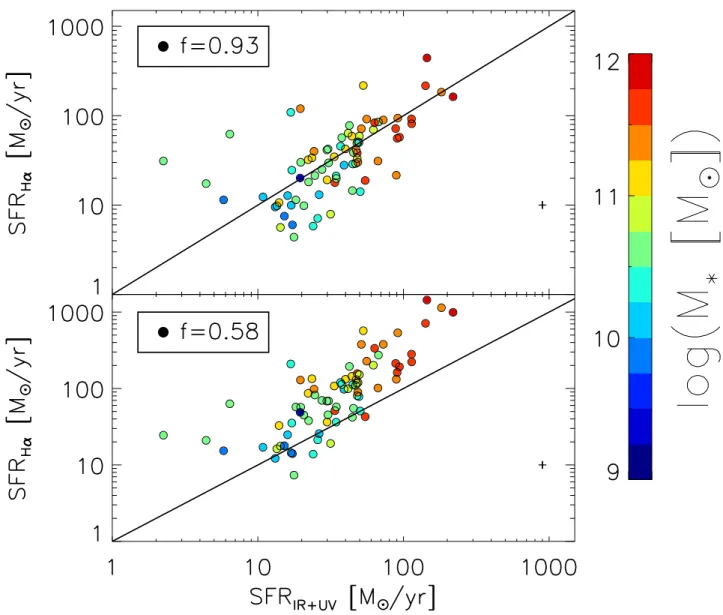
Fig. 11.Comparison between SFRIR+UVand SFRHαwhen varying the dust correction for the Hα emission. The lower panel shows the case where
LHαare corrected for dust attenuation by using the classical prescription of Calzetti ( f = 0.58) while in the upper panel the Hα luminosities are
corrected with our dust correction ( f = 0.93). The black solid line is the 1:1 correlation line and the different colors indicate the stellar masses, as indicated in the vertical color bar. The lowest part of each panel also shows the median errors on the SFR measurements.
5.3. Extra extinction from the f-factor
Following the formalism of Sect.5.1, we evaluated the f -factor as a function of the color excess on the continuum by using the ratio SFRHα,uncorr/SFRUV,uncorr and the two measurements
of the color excess on stellar continuum, Estar,β(B − V) and
Estar,IRX(B − V). To derive the f -factor we fit a linear
func-tion y = s × x to the data points through a minimization of a weighted χ2 (i.e., a least square fit obtained by weighting
each data point for its error in both the x and y axes), where y = log(SFRHα,uncorr/SFRUV,uncorr) and x = Estar(B − V). To
obtain this fit we used the routine mpfit.pro, and took care of checking the result by a MC simulation by inserting a scatter in the x-coordinate value for each datapoint. The f -factor is then finally obtained from the slope s of the best-fit line as
f = 0.4 × k(Hα)
0.4 × k(UV) − s· (12)
The uncertainty for the f -factor was estimated by propagating the error on the best-fit parameter s.
Figure 10 reports SFRHα,uncorr/SFRUV,uncorr as a function
of the continuum color excess. The red solid line in Fig. 10
corresponds to Eq. (7) with f = 0.93 (±0.065), which is the best-fit value from our data distribution. We therefore found that the f -factor required to match SFRHα and SFRUV in our
sam-ple is larger than the local value ( f = 0.58, blue dashed line in Fig.10) and turns out to also be higher than the values computed byKashino et al.(2013) on a sample with slightly higher z and different selection criteria (f =0.69 and 0.83, black dot-dashed and green dot-dot-dashed lines in Fig.10respectively).
The value of the f -factor does not change using either Estar,β(B − V) or Estar,IRX(B − V): this result is in line with the
high correlation of these two measurements, as seen in Fig.9.
5.4. Testing the dust correction: comparison between SFRHα
and SFRIR+UV
We tested the reliability of our extinction correction in Fig.11, where we compared the SFRIR+UVwith the SFRHα, corrected for
dust extinction using both the prescriptions derived in this work (i.e., Estar,IRX(B − V) and f = 0.93, upper panel) and byCalzetti
et al.(2000) for local galaxies (Estar,IRX(B − V) and f = 0.58,
Fig. 12.AHαas a function of stellar masses. The black filled circles are
the sources at z < 1 while red filled squares are objects with z > 1. The attenuation is computed from Estar,IRX(B − V) by using f = 0.93. The
gray filled circles are the median values of AHαin three mass bins (M?<
3×10¹⁰M
, 3×10¹⁰≤ M?< 1.7×10¹¹M , M?≥ 1.7×10¹¹M ) and the
errorbars are the median scatter for AHαand M?in each mass bin. The
two vertical dashed lines highlight the mass bins (M? < 3 × 10¹⁰ M ,
3 × 10¹⁰≤ M
?< 1.7 × 10¹¹M , M?≥ 1.7 × 10¹¹M ).
SFRHα and SFRIR+UV is obtained by applying our correction
factor with a median ratio SFRHα/SFRIR+UV = 0.88 and a
me-dian relative scatter |SFRIR+UV− SFRHα|/(1+SFRIR+UV)= 0.38.
In contrast, the Calzetti et al. prescription would lead to over-estimate the SFRHα by a factor up to 3.3 above SFRIR+UV >
50 M /yr. We emphasize that our recipe for the nebular dust
at-tenuation seems to “fail” for the tail of objects with SFRIR+UV∈
[10−20] M /yr and M?∼ 1010M (light blue points in Fig.11).
For these sources our dust correction underestimates the SFRHα
with respect to SFRIR+UV, while using the Calzetti prescription
the two SFRs are in slightly better agreement. This could imply that the f -factor is an increasing function of SFR and M?.
However, the disagreement between SFR indicators at SFRIR+UV <∼ 20 M /yr can be due also to an overestimate
of SFRIR+UV rather than a problem of the dust correction. At
lower M?and SFRs in fact, the contamination to the heating of
dust by an older stellar population (the so-called “cirrus” compo-nent, e.g.Kennicutt et al. 2009) became not-negligible, making it possible to overestimate LIR. Finally, the trend seen in Fig.
ref-compareSFR could also be a consequence of the selection crite-rion used in this work, considering that SFRIR+UV∼ 15 M /yr is
the value that corresponds to the 3σ flux limit at 160 µm at z ∼ 1 as estimated using the median SEDs ofMagdis et al.(2012) (see also Fig.2of Sect.2.5).
5.5. AHαvs. M?
Figure 12shows the relationship between the attenuation AHα
and stellar masses. Here we converted the continuum attenua-tion Estar,IRX(B − V) to AHαby using f = 0.93 and the k(λ) from
Calzetti et al.(2000). Despite the high dispersion of the data, we can observe an excess of AHαat the highest masses with respect
to the local relationship of Garn & Best(2010) (green dashed line in Fig.12). We also report the relationship ofKashino et al. (2013), derived at z ∼ 1.6 (blue solid line). Figure 12 repre-sents the median values of AHα obtained in three M? bins as
reported in the figure. The errorbars are the median scatter of
Fig. 13.SFRHαversus M?with LHαcorrected by dust with our recipe.
The blue solid line reports the MS relationship fromElbaz et al.(2007) at z= 1, and the blue dashed line is the corresponding 4×MS. The black filled circles are the sources at z < 1, while the red filled squares are the objects at z > 1. The median errors for M?and SFRHαare reported in
the lower part of the plot on the right.
AHαand M?in each bin. Within the large scatter in the data, the
median values in each bin are consistent with both the local and the higher-z relationships, in agreement with the results ofIbar et al.(2013). Of course, there may be selection effects in opera-tion in the graph that disfavor the detecopera-tion of galaxies with high values of AHα, which may be more important for the lower mass
objects with intrinsically faint Hα flux. Our combined selection requiring detection of the Hα line may be somewhat exposed to such an effect. To confirm that an evolution with z exists in the dust properties of star-forming galaxies it would be necessary to have deeper observations for the most attenuated galaxies. This aspect of the analysis will be investigated in a later paper.
5.6. Main sequence at z ∼ 1
In Fig.13we report an updated version of the relation between the stellar mass and the SFR, already presented in Fig.2, where SFR is now computed from the Hα luminosities, corrected for dust extinction according to our reference dust correction. As al-ready mentioned in Sect.2.5, our sources do not span the overall range covered by the star-forming main sequence population at z ∼ 1, since our far-IR selection favor the detection of sources with SFR > 10−20 M /yr. However, we note that above stellar
masses on the order of 3 × 10¹⁰ M , our sample is basically
rep-resentative of a mass-selected sample that traces the underlying MS at the same redshift.
6. Caveats: the many faces of the f -factor
Values of the f -factor estimated in the literature range from 0.44 to ∼1 , as shown in Table3, and in this section we briefly dis-cuss the likely origins of these differences. An f -factor less than unity is currently interpreted as implying more average obscura-tion affecting the line-emitting regions (HII regions) compared to the average obscuration affecting the hot stars emitting the UV continuum, i.e., f , 1 would be the result of a geometri-cal effect with the spacial distribution of line emitting regions
being different from that of continuum emitting stars. Actually, the reality may be somewhat more complicated.
First of all, the f -factor can be derived in two radically dif-ferent ways: either by comparing two extinctions or two SFRs. In the former case the Hα extinction derived from the Balmer decrement is compared to the extinction in the UV as derived from either the UV slope or from Eq. (10). Then one has to adopt one specific reddening law k(λ). In the latter case, the f -factor is estimated by enforcing equality between the SFR derived from the Hα flux with the SFR derived from another indicator, such as SFR(UV), SFR(UV+IR), or SFR from SED fitting.
When the f -factor is derived by comparing Hα and UV ex-tinction, then the result depends on the adopted reddening law k(λ), so it at once reflects both the mentioned geometrical ef-fect and possible departures from the adopted reddening law. As well known, the reddening law is not universal, not even within the Local Group. These two contributions to determine the value of f can barely be disentangled. When the f -factor is derived by forcing agreement between SFR(Hα) and the SFR from another indicator, then it becomes a fudge factor to compensate for the relative biases of the two SFR estimators, neither of which will be perfect.
Moreover, the measured Hα flux is subject to dust absorp-tion in two distinct ways: first, each Hα photon has a probability 10−0.4AHα of escaping the galaxy, but second, dust absorption in
the Lyman continuum reduces the number of produced Hα pho-tons by a factor 10−0.4ALyman−cont., where A
Lyman−cont. is the
extinc-tion in the Lyman continuum. With few excepextinc-tions (e.g.Boselli et al. 2009), this second aspect is generally ignored, in the hope that an empirical calibration of SFRs may also subsume in it this part of the involved physics. In any event, the resulting f -factor depends on the actual extinction law of each galaxy, extending from the optical all the way to the Lyman continuum, on the geometry of the emitting regions, as well as on the relative sys-tematic biases in the relations connecting SFRs to observables.
Besides these aspects, derived f values can also depend on the specific galaxy sample from which it is derived. For example, in our approach the far-IR selection criterion leads to selecting objects with strong levels of dust obscuration in the UV. The other requirement is to select objects with a strong Hα emission (Fobs(Hα) > 2.87 × 10⁻¹⁷erg/s and S/N higher than ∼3), hence
with lower levels of Hα attenuation. The two selection criteria partially conflict with each other and combined favor sources with Eneb(B − V) ∼ Estar(B − V). To understand how the selection
criterion influences the results we can compare our analysis with the work ofKashino et al.(2013). Our analysis was performed following the same approach as in Kashino et al.(2013), but our sample has a different selection criterion and size (168 sBzK galaxies for Kashino, 79 far-IR sources in this work), and we obtained an f = 0.93, which is 35% larger than the Kashino result. In the case of rest-frame UV-selected galaxies, such as in Erb et al.(2006), this bias favors galaxies with low extinction, which may result in a different f value compared to the case of samples, also including highly reddened galaxies.
All of these considerations imply that different indicators lead to different estimates of the f -factor. For example, if we consider the ratio SFRuncHα/SFRIR+UV, we get (see, e.g., Eq. (7))
S FRHα,uncorr
S FRIR+UV
= 10−0.4AHα= 10−0.4Estar(B−V)f k(Hα). (13)
Our data would imply f ' 0.85 in this case, which is, however, not significantly different from our best guess of f ' 0.93.
Table 2. Summary of the values obtained for the f -factor as a function of the assumed reddening curve k(λ).
k(UV) k(Hα) f-factor
Calzetti et al.(2000) Calzetti et al.(2000) 0.93
Calzetti et al.(2000) Fitzpatrick(1999) 0.66
Reddy et al.(2015) Reddy et al.(2015) 0.96
Reddy et al.(2015) Fitzpatrick(1999) 1.19
Notes. the first column is the k(λ) assumed to compute the UV attenu-ation at 1600 Å, the second column is the k(λ) used to compute the Hα attenuation while the last column is the f -factor, obtained from Eq. (12).
Also the estimate of Estar(B − V) and its errors influences the
estimate of the f -factor, leading to results that can vary from f ∼ 0.4 to a value greater than 1.
The last point to consider is again the reddening law k(λ) assumed in the analysis. In the literature one finds very di ffer-ent trends for k(λ), such as the presence of a bump at ∼2200 Å (Fitzpatrick 1999, for the LMC) or a smoother trend (Calzetti et al. 2000, for a starburst galaxy), and also very different values for its normalization RV ≡ AV/Estar(B − V), which vary from 3.1
(Cardelli et al. 1989) to 4.05 (Calzetti et al. 2000). At redshift ∼2, both galaxies with and without the 2200 Å bump appear to coexist (Noll et al. 2009). The shape and the normalization of the assumed k(λ) strongly influences the value of f, both for direct or indirect measurements. As an exercise we derived the f -factor using different k(λ) expressions in Eq. (12). Table2summarizes the results, showing that the value of the f -factors ranges from ∼0.7 to ∼1.2.
In summary, the f -factor may offer a fair measure of the rel-ative extinction of emission lines and the stellar continuum, still however relying on ingredients that are not completely well de-fined and understood.
7. Summary and conclusions
In this work we analyzed the near-IR spectra of 79 star-forming galaxies at z ∈ [0.7−1.5], acquired from the 3D-HST survey . The sources were selected in the far-IR from the Herschel/PACS observations: the PACS catalogs were associ-ated with the 3D-HST observations using the IRAC positions of the PACS sources. From the near-IR spectra we measured the Hα fluxes and the spectroscopic redshifts of the whole sample.
We computed the SEDs with the MAGPHYS software, using data from near-UV to far-IR including the GALEX-NUV, the GOODS-MUSIC optical to mid-IR catalog, the IRS-16 µm and the far-IR photometry from Herschel PACS and SPIRE (i.e., at 70, 100, 160, 250, 350 and 500 µm). From the SEDs we derived the stellar masses M?, the bolometric infrared luminosities LIR,
the UV luminosities LUV, and the UV slope β.
We then evaluated the color excess Estar(B − V) from the
IRX= LIR/LUV ratio and from the UV slope β and found that
these two quantities are in good agreement. In our sample the color excess on the stellar continuum ranges from Estar(B − V) ∼
0.1 mag to Estar(B − V) ∼ 1.1 mag.
We computed the dust attenuation on the Hα emission Eneb(B−V) as a function of Estar(B−V) by comparing the SFRHα
and the SFRUV, both uncorrected for extinction. We obtained
that the f -factor, which parametrizes the differential extinction on the nebular lines, is f = Estar(B − V)/Eneb(B − V)= 0.93 ±
0.06. This result is consistent within the errorbars with the anal-ysis ofKashino et al.(2013) from the Balmer Decrement and of
Table 3. Different values of f obtained from literature.
Author f zrange Sample Method
Calzetti et al.(2000) 0.44 (0.58) 0.003−0.05 starburst galaxies Balmer decrement
Kashino et al.(2013) 0.83 ± 0.10 1.4−1.7 sBzk galaxies Balmer decrement (stacked spectra)
" 0.69 ± 0.02 " " Hα to UV SFRs
Wuyts et al.(2011) 0.44 0−3 Ksselected galaxies SFR indicators
Price et al.(2014) 0.55 ± 0.16 1.36−1.5 MS star forming galaxies Balmer decrement (stacked spectra)
Pannella et al.(2015) 0.58 <1 UVJ selected galaxies comparison between AUV− M?/AHα− M?
" 0.77 1 " "
" 1 >1 " "
Valentino et al.(2015) 0.74 ± 0.05 2 CL J1449+0856 Balmer decrement (stacked spectra)
Erb et al.(2006) 1 2 rest-frame UV selected galaxies matching UV and Hα SFRs
Reddy et al.(2010) 1 1.5−2.6 Lyman Break Galaxies matching X-ray, UV and Hα SFRs
This work 0.93 ± 0.06 0.7−1.5 far-IR selected galaxies Hα to UV SFRs
Notes. Table also specifies the redshift ranges (third column of Table3), the types of sample, and the methods implied to measure the differential
extinction on nebular lines (fourth and fifth columns of Table3, respectively).
Pannella et al.(2015), performed in a similar redshift range. Our analysis is also consistent with the results ofErb et al. (2006) andReddy et al.(2010) performed at higher z, as summarized in Table3, which collect a list of results from others works. The good agreement found in our sample between the SFRIR+UVand
the SFRHαcorrected for extinction using our recipe further
con-firm our results.
From our dust correction we then computed the attenuation AHαas a function of M?. We found that AHαis increasing with
M?and this trend seems to diverge from the local relationship:
our sources shows an excess of AHαwith respect to the
relation-ship ofGarn & Best(2010) for M? >∼ 1011 M , suggesting an
evolution in the dust properties of star-forming galaxies with z. In conclusion we found that the level of differential extinc-tion required to match the SFRHα with the SFRIR+UV is lower
than in the local Universe, thus AHα∼ AUVfor the sources in our
sample. The value of the f -factor seems to be related to the phys-ical properties of the sample rather than be dependent on z. The trends of Figs. 11and12suggest that the Hα extinction (thus the f -factor) is a function of SFR and M?. In particular we no-tice that in Fig.11our dust correction underestimate SFRHαwith
respect to SFRIR+UV for sources with SFR <∼ 20 M /yr: these
sources require a lower value of f, similar to the local f = 0.58. This trend could be explained by the two components model of dust sketched in Fig. 5 ofPrice et al.(2014). A galaxy with high sSFR is supposed to have a high number of OB stars, which are located inside the optically thick birth cloud: in this case these massive stars dominate both the UV-continuum and the Hα emissions, so the level of attenuation for the continuum and the nebular emission will be similar (AUV ∼ AHα). On the other
hand, for a galaxy with low sSFR, the number of OB stars will be lower, so in this case the optical-UV continuum is mainly produced by the less massive stars that are located both in the birth cloud and in the diffuse ISM: in this case AHα> AUVsince
the Hα emission is produced in a different and more dust-dense region with respect to the continuum.
In this paper we do not examine the consequences of this modellistic approach in depth for the reasons discussed in the previous section. We defer to a future paper a more detailed anal-ysis of the extinction properties of star-forming galaxies based on the “Intensive Program” (S12B-045, PI J. Silverman) with the FMOS spectrograph at the Subaru Telescope in the COSMOS field (Silverman et al. 2015).
Acknowledgements. We thank the anonymous referee for a careful reading of the manuscript an for valuable comments. A.P., G.R., and A.F.
acknowl-edge support from the Italian Space Agency (ASI) (Herschel Science Contract I/005/07/0). We are grateful to Antonio Cava for the improvement of the IDL code used for the spectral analysis and Robert Kennicutt and Naveen Reddy for their comments. We also thank Mattia Negrello for his help with the error analy-sis and his comments. This work is based on observations taken by the 3D-HST Treasury Program (GO 12177 and 12328) with the NASA/ESA HST, which is operated by the Association of Universities for Research in Astronomy, Inc., un-der NASA contract NAS5-26555.
References
Akritas, M. G., & Bershady, M. A. 1996,ApJ, 470, 706 Baldwin, J. A., Phillips, M. M., & Terlevich, R. 1981,PASP, 93, 5 Berta, S., Magnelli, B., Nordon, R., et al. 2011,A&A, 532, A49 Berta, S., Lutz, D., Santini, P., et al. 2013,A&A, 551, A100 Boselli, A., Boissier, S., Cortese, L., et al. 2009,ApJ, 706, 1527 Brammer, G., van Dokkum, P. G., Franx, M., et al. 2012,ApJs, 200, 13 Bruzual, G., & Charlot, S. 2003,MNRAS, 344, 1000
Buat, V., Noll, S., Burgarella, D., et al. 2012,A&A, 545, A141 Calzetti, D. 2001,NewAR, 45, 601
Calzetti, D., Kinney, A. L., & Storchi-Bergmann, T. 1994,ApJ, 429, 582 Calzetti, D., Armus, L., Bohlin, R. C., et al. 2000,ApJ, 533, 682 Cardelli, J. A., Clayton, G. C., & Mathis, J. S. 1989,ApJ, 345, 245 Chabrier, G. 2003,PASP, 115, 763
Charlot, S., & Fall, S. M. 2000,ApJ, 539, 718
Cid Fernandes, R., Mateus, A., Sodré, L., Stasi´nska, G., & Gomes, J. M. 2005, MNRAS, 358, 363
Cimatti, A., Cassata, P., Pozzetti, L., et al. 2008,A&A, 482, 21 da Cunha, E., Charlot, S., & Elbaz, D. 2008,MNRAS, 388, 1595
Domínguez Sánchez, H., Bongiovanni, A., Lara-López, M. A., et al. 2014, MNRAS, 441, 2
Elbaz, D., Daddi, E., Le Borgne, D., et al. 2007,A&A, 468, 33 Erb, D. K., Steidel, C. C., Shapley, A. E., et al. 2006,ApJ, 647, 128 Fanelli, M. N., O’Connell, R. W., & Thuan, T. X. 1988,ApJ, 334, 665 Fioc, M., & Rocca-Volmerange, B. 1997,A&A, 326, 950
Fitzpatrick, E. L. 1999,PASP, 111, 63
Förster Schreiber, N. M., Genzel, R., Bouché, N., et al. 2009, ApJ, 706, 1364
Garn, T., & Best, P. N. 2010,MNRAS, 409, 421
Grazian, A., Fontana, A., de Santis, C., et al. 2006,A&A, 449, 951 Grogin, N. A., Kocevski, D. D., Faber, S. M., et al. 2011,ApJS, 197, 35 Gruppioni, C., Pozzi, F., Rodighiero, G., et al. 2013,MNRAS, 432, 23 Ibar, E., Sobral, D., Best, P. N., et al. 2013,MNRAS, 434, 3218 Kashino, D., Silverman, J. D., Rodighiero, G., et al. 2013,ApJ, 777, L8 Kennicutt, Jr., R. C. 1998,ARAA, 36, 189
Kennicutt, Jr., R. C., Hao, C.-N., Calzetti, D., et al. 2009,ApJ, 703, 1672 Koekemoer, A. M., Faber, S. M., Ferguson, H. C., et al. 2011,ApJs, 197, 36 Levenson, L., Marsden, G., Zemcov, M., et al. 2010,MNRAS, 409, 83 Lutz, D., Poglitsch, A., Altieri, B., et al. 2011,A&A, 532, A90 Madau, P., & Dickinson, M. 2014,ARA&A, 52, 415
Magdis, G. E., Daddi, E., Béthermin, M., et al. 2012,ApJ, 760, 6 Magnelli, B., Elbaz, D., Chary, R. R., et al. 2009,A&A, 496, 57
Markwardt, C. B. 2009, in Astronomical Data Analysis Software and Systems XVIII, eds. D. A. Bohlender, D. Durand, & P. Dowler,ASP Conf. Ser., 411, 251
Mas-Hesse, J. M., & Kunth, D. 1999,A&A, 349, 765
Mayya, Y. D., Bressan, A., Rodríguez, M., Valdes, J. R., & Chavez, M. 2004, ApJ, 600, 188
Meurer, G. R., Heckman, T. M., & Calzetti, D. 1999,ApJ, 521, 64 Morris, A. M., Kocevski, D. D., Trump, J. R., et al. 2015,AJ, 149, 178 Noeske, K. G., Weiner, B. J., Faber, S. M., et al. 2007,ApJ, 660, L43 Noll, S., Burgarella, D., Giovannoli, E., et al. 2009,A&A, 507, 1793 Nordon, R., Lutz, D., Genzel, R., et al. 2012,ApJ, 745, 182 Nordon, R., Lutz, D., Saintonge, A., et al. 2013,ApJ, 762, 125 Oliver, S. J., Bock, J., Altieri, B., et al. 2012,MNRAS, 424, 1614 Oteo, I., Bongiovanni, Á., Magdis, G., et al. 2014,MNRAS, 439, 1337 Pannella, M., Elbaz, D., Daddi, E., et al. 2015,ApJ, 807, 141 Price, S. H., Kriek, M., Brammer, G. B., et al. 2014,ApJ, 788, 86 Reddy, N. A., Erb, D. K., Pettini, M., et al. 2010,ApJ, 712, 1070 Reddy, N., Dickinson, M., Elbaz, D., et al. 2012,ApJ, 744, 154 Reddy, N. A., Kriek, M., Shapley, A. E., et al. 2015,ApJ, 806, 259 Rodighiero, G., Daddi, E., Baronchelli, I., et al. 2011,ApJ, 739, L40 Rodighiero, G., Renzini, A., Daddi, E., et al. 2014,MNRAS, 443, 19
Roseboom, I. G., Oliver, S. J., Kunz, M., et al. 2010,MNRAS, 409, 48 Salpeter, E. E. 1955,ApJ, 121, 161
Santini, P., Fontana, A., Grazian, A., et al. 2009,VizieR Online Data Catalog: J/A+A/504/751
Schmidt, K. B., Rix, H.-W., da Cunha, E., et al. 2013,MNRAS, 432, 285 Silverman, J. D., Kashino, D., Arimoto, N., et al. 2015,ApJS, 220, 12 Skelton, R. E., Whitaker, K. E., Momcheva, I. G., et al. 2014, ApJS, 214,
24
Steidel, C. C., Rudie, G. C., Strom, A. L., et al. 2014,ApJ, 795, 165 Talia, M., Cimatti, A., Pozzetti, L., et al. 2015,A&A, 582, A80 Teplitz, H. I., Charmandaris, V., Chary, R., et al. 2005,ApJ, 634, 128 Valentino, F., Daddi, E., Strazzullo, V., et al. 2015,ApJ, 801, 132 Viero, M. P., Wang, L., Zemcov, M., et al. 2013,ApJ, 772, 77 Whitaker, K. E., Franx, M., Leja, J., et al. 2014,ApJ, 795, 104 Wuyts, S., Förster Schreiber, N. M., Lutz, D., et al. 2011,ApJ, 738, 106 Wuyts, S., Förster Schreiber, N. M., Nelson, E. J., et al. 2013,ApJ, 779, 135 Xue, Y. Q., Luo, B., Brandt, W. N., et al. 2011,ApJS, 195, 10
Yoshikawa, T., Akiyama, M., Kajisawa, M., et al. 2010,ApJ, 718, 112 Zahid, H. J., Geller, M. J., Kewley, L. J., et al. 2013,ApJ, 771, L19 Zahid, H. J., Kashino, D., Silverman, J. D., et al. 2014,ApJ, 792, 75
Fig. A.1. Linear fit (red line) to the best-fit SED in the plane log(λ), log(Fλ).
Appendix A: Computation of the UV spectral slope A.1. β from the best-fit SED
The UV slope is derived from a linear fit to the model best-fit SED in the wavelength range λ ∈ [1250−2600] Å, lacking ob-servations in this rest-frame range for the majority of the sample. An example of the fit is shown in Fig.A.1. The errors related to the βmodel, i.e., the UV slope derived from the MAGPHYS SED,
are computed from the linear fit. A.2. β from the observed photometry
To test the validity of the estimate of βmodel we also computed
the UV-slope from the observed data, when the photometric coverage in the rest-frame range of interest is available. We interpolated the observed photometry in the rest-frame range λ ∈ [1200−3500] Å, following the method described inNordon et al.(2013). The photometric UV-spectral slope is defined as βphot=
−0.4(M1− M2)
log(λ1/λ2)
− 2 (A.1)
where M1and M2are the AB magnitudes at wavelengths λ1 =
1600 Å and λ2= 2800 Å.
The rest-frame 1600 Å and 2800 Å magnitudes (M1600and
M2800) were estimated by interpolating between the available
photometric bands. To derive M1600we used the filters between
rest-frame λ ∈ [1200−2800] Å and interpolated the flux at 1600 Å (converted to AB magnitudes) by fitting a linear function between the observed photometric bands. To derive M2800we
se-lected the filters that observe the rest frame λ ∈ [1500−3500] Å. FigureA.2shows an example for the computation of M1600and
M2800for a source that has the required photometric coverage.
FigureA.3shows the case in which we did not have the cover-age in the rest frame. The βphotwas computed for 13 sources. We
computed the errors for βphotby using a set of MC simulations:
we randomly varied the observed photometry within the error-bars and then computed the interpolation for each set of sim-ulated values of the observed photometry. The 1σ uncertainty on βphot was then estimated from the width of the probability
distribution function of the simulated values, assuming that this distribution has a Gaussian shape. The median error on βphotwas
added in quadrature to the error of βmodelso thus the error for the
UV-slope is σ2
β,i= σ2βmodel,i+ median(σ
2 βphot,i).
Fig. A.2.Method for computing βphotfor the source 3213 (ID MUSIC).
The figure also specifies the redshift of the source. The black open dia-monds are the observed photometry, connected with a linear interpola-tion (black solid line). The green vertical lines highlight the rest-frame spectral range considered to compute M1, while the blue vertical lines
outline the range for the computation of M2. The two dash-dot red lines
show the positions of 1600 Å and 2800 Å rest frame, respectively.
Fig. A.3. As in Fig. A.2, without the photometric coverage to derive βphot.
A.3.βphot vs.βmodel
The UV spectral slope is model-dependent, since it is obtained from a fit to the SED: to verify the validity of our measurements we compared βmodel to βphot for the 13 sources that have the
required photometric coverage in the UV spectrum. The SEDs were recomputed, but in this case excluding the photometric bands in the UV rest-frame spectral range, because we want to compare a value that strongly depends on the model to those constrained by the observed data. The correlation between βmodel
and βphotis shown in Fig.A.4: the agreement between the two
estimates is quite good, when also considering the poor statis-tic, and confirms the reliability of βmodel derived by fitting the
Fig. A.4. Comparison between βmodel, derived from the SED fitting,
and βphot, computed by fitting the observed photometry, for the
15 sources with photometric coverage in the rest-frame range λ ∈ [1200−3500]Å. The blue line is the 1:1 line. The linear Pearson cor-relation coefficient is r = 0.96.
Appendix B: Main parameters of the sample
TableB.1summarizes the MUSIC ID, the coordinates, the red-shift measured from the 3D-HST near-IR spectra, the observed Hα luminosity LHα,obscorrected for the aperture as explained in
Sect.3.2, the infrared luminosity LIR, the observed UV


![Fig. A.4. Comparison between β model , derived from the SED fitting, and β phot , computed by fitting the observed photometry, for the 15 sources with photometric coverage in the rest-frame range λ ∈ [1200−3500]Å](https://thumb-eu.123doks.com/thumbv2/123doknet/13360751.403072/16.892.85.426.126.380/comparison-derived-fitting-computed-observed-photometry-photometric-coverage.webp)
