HAL Id: hal-01886165
https://hal.inria.fr/hal-01886165
Submitted on 2 Oct 2018
HAL is a multi-disciplinary open access
archive for the deposit and dissemination of
sci-entific research documents, whether they are
pub-lished or not. The documents may come from
teaching and research institutions in France or
abroad, or from public or private research centers.
L’archive ouverte pluridisciplinaire HAL, est
destinée au dépôt et à la diffusion de documents
scientifiques de niveau recherche, publiés ou non,
émanant des établissements d’enseignement et de
recherche français ou étrangers, des laboratoires
publics ou privés.
To cite this version:
Jean-Daniel Boissonnat, Siddharth Pritam, Divyansh Pareek. Strong Collapse for Persistence. ESA
2018 - 26th Annual European Symposium on Algorithms, Aug 2018, Helsinki, Finland. pp.67:1–67:13,
�10.4230/LIPIcs�. �hal-01886165�
Jean-Daniel Boissonnat
1, Siddharth Pritam
2, and Divyansh
Pareek
31 Université Côte d’Azur, INRIA, France Jean-Daniel.Boissonnat@inria.fr
2 Université Côte d’Azur, INRIA, France siddharth.pritam@inria.fr
3 Université Côte d’Azur, INRIA, France divyanshpareek21@gmail.com
Abstract
We introduce a fast and memory efficient approach to compute the persistent homology (PH) of a sequence of simplicial complexes. The basic idea is to simplify the complexes of the input sequence by using strong collapses, as introduced by J. Barmak and E. Miniam [1], and to compute the PH of an induced sequence of reduced simplicial complexes that has the same PH as the initial one. Our approach has several salient features that distinguishes it from previous work. It is not limited to filtrations (i.e. sequences of nested simplicial subcomplexes) but works for other types of sequences like towers and zigzags. To strong collapse a simplicial complex, we only need to store the maximal simplices of the complex, not the full set of all its simplices, which saves a lot of space and time. Moreover, the complexes in the sequence can be strong collapsed independently and in parallel. As a result and as demonstrated by numerous experiments on publicly available data sets, our approach is extremely fast and memory efficient in practice. 1998 ACM Subject Classification Dummy classification – please refer to http://www.acm.org/ about/class/ccs98-html
Keywords and phrases Computational Topology, Topological Data Analysis, Strong Collapse, Persistent homology
Digital Object Identifier 10.4230/LIPIcs...
1
Introduction
In this article, we address the problem of computing the Persistent Homology (PH) of a given sequence of simplicial complexes (defined precisely in Section 4) in an efficient way. It is known that computing persistence can be done in O(nÊ) time, where n is the total number
of simplices and Ê Æ 2.4 is the matrix multiplication exponent [25, 17]. In practice, when dealing with massive and high-dimensional datasets, n can be very large (of order of billions) and computing PH is then very slow and memory intensive. Improving the performance of PH computation has therefore become an important research topic in Computational Topology and Topological Data Analysis.
Much progress has been accomplished in the recent years in two directions. First, a number of clever implementations and optimizations have led to a new generation of software for PH computation [37, 39, 40, 41]. Secondly, a complementary direction has been explored
This research has received funding from the European Research Council (ERC) under the European Union’s Seventh Framework Programme (FP/2007- 2013) / ERC Grant Agreement No. 339025 GUDHI (Algorithmic Foundations of Geometry Understanding in Higher Dimensions).
© Jean-Daniel Boissonnat, Siddharth Pritam, and Divyansh Pareek; licensed under Creative Commons License CC-BY
Leibniz International Proceedings in Informatics
to reduce the size of the complexes in the sequence while preserving (or approximating in a controlled way) the persistent homology of the sequence. Examples are the work of Mischaikow and Nanda [8] who use Morse theory to reduce the size of a filtration, and the work of D≥otko and Wagner who use simple collapses [13]. Both methods compute the exact PH of the input sequence. Approximations can also be computed with theoretical guarantees. Approaches like interleaving smaller and easily computable simplicial complexes, and sub-sampling of the point sample works well upto certain approximation factor [21, 12, 10, 9].
In this paper, we introduce a new approach to simplify the complexes of the input sequence which uses the notion of strong collapse introduced by J. Barmak and E. Miniam [1]. Specifically, our approach can be summarized as follows: Given a sequence Z : {K1≠æf1
K2Ω≠ Kg2 3≠æ · · ·f3 ≠≠≠≠æ Kf(n≠1) n} of simplicial complexes Kiconnected through simplicial maps
{fi
≠æ orΩ≠}. We independently strong collapse the complexes of the sequence to reach agj sequence Zc : {Kc 1 fc 1 ≠æ Kc 2 gc 2 Ω≠ Kc 3 fc 3 ≠æ · · · f c (n≠1) ≠≠≠≠æ Kc
n}, with induced simplicial maps { fc
i
≠æ or
gc j
Ω≠} (defined in Section 4). The complex Kc
i is called the core of the complex Ki and we
call the sequence Zc the core sequence of Z. We show that one can compute the PH of
the sequence Z by computing the PH of the core sequence Zc, which is of much smaller size.
Our method has some similarity with the work of Wilkerson et. al. [5] who also use strong collapses to reduce PH computation but it differs in three essential aspects: it is not limited to filtrations (i.e. sequences of nested simplicial subcomplexes) but works for other types of sequences like towers and zigzags. It also differs in the way the strong collapses are computed and in the manner PH is computed.
A first central observation is that to strong collapse a simplicial complex K, we only need to store its maximal simplices (i.e. those simplices that have no coface). The number of maximal simplices is smaller than the total number of simplices by a factor that is exponential in the dimension of the complex. It is linear in the number of vertices for a variety of complexes [32]. Working only with maximal simplices dramatically reduces the time and space complexities compared to the algorithm of [4]. We prove that the complexity of our algorithm is O(v2
0d+ m2 0d). Here d is the dimension of the complex, v is the
number of vertices, m is the number of maximal simplices and 0 is an upper bound on the
number of maximal simplices incident to a vertex. 0is a small fraction of the number of
maximal simplices [31].
We now consider PH computation. All PH algorithms take as input a full representation of the complexes and their complexity is polynomial in the total number of simplices of the complexes. We thus have to convert the representation by maximal simplices used for the strong collapses into a full representation of the complexes, which takes exponential time in the dimension (of the collapsed complexes). This exponential burden is to be expected since it is known that computing PH is NP-hard when the complexes are represented by their maximal faces [7]. Nevertheless, we demonstrate in this paper that strong collapses combined with known persistence algorithms lead to major improvements over previous methods to compute the PH of a sequence. This is due in part to the fact that strong collapses reduce the size of the complexes on which persistence is computed. The following factors also contribute: – The collapses of the complexes in the sequence can be performed independently and in parallel. This is due to the fact that strong collapses can be expressed as simplicial maps unlike simple collapses [30].
– The size of the complexes in a sequence does not grow by much in terms of maximal simplices, as observed in many practical cases. As a consequence, the time to collapse the
a clear advantage over methods that use a full representation of the complexes and suffer an increasing cost as i increases.
As a result, our approach is extremely fast and memory efficient in practice as demon-strated by numerous experiments on publicly available data sets.
An outline of this paper is as follows. Section 2 recalls the basic ideas and constructions related to simplicial complexes and strong collapses. We describe our core algorithm in Section 3. In Section 4, we prove that zigzag modules are preserved under strong collapse. In Section 5, we provide experimental results.
2
Preliminaries
In this section, we provide a brief review of the notions of simplicial complex and strong collapse as introduced in [1]. We assume some familiarity with basic concepts like homotopic maps, homotopy type, homology groups and other algebraic topological notions. Readers can refer to [29] for a comprehensive introduction of these topics.
Simplex, simplicial complex and simplicial map : An abstract simplicial complex K
is a collection of subsets of a non-empty finite set X, such that for every subset A in K, all the subsets of A are in K. From now on we will call an abstract simplicial complex simply a simplicial complex or just a complex. An element of K is called a simplex. An element of cardinality k + 1 is called a k-simplex and k is called its dimension. A simplex is called maximal if it is not a proper subset of any other simplex in K. A sub-collection L of K is called a subcomplex, if it is a simplicial complex itself. L is a full subcomplex if it contains all the simplices of K that are spanned by the vertices (0-simplices) of the subcomplex L.
A vertex to vertex map  : K æ L between two simplicial complexes is called a simplicial
map, if the images of the vertices of a simplex always span a simplex. Simplicial maps
are thus determined by the images of the vertices. In particular, there are a finite number of simplicial maps between two given finite simplicial complexes. Simplicial maps induce continuous maps between the underlying geometric realisations of the simplicial complexes.
Dominated vertex: Let ‡ be a simplex of a simplicial complex K, the closed star of ‡ in K, stK(‡) is a subcomplex of K which is defined as follows, stK(‡) := {· œ K| · fi “ œ
K; where “ ™ ‡}. The link of ‡ in K, lkK(‡) is defined as the set of simplices in stK(‡)
which do not intersect with ‡, lkK(‡) := {· œ stK(‡)|· fl ‡ = ÿ}.
Taking a join with a vertex transforms a simplicial complex into a simplicial cone. Formally if L is a simplicial complex and a is vertex not in L then the simplicial cone aL is defined as, aL := {a, · | · œ L or · = ‡ fi a; where ‡ œ L}. A vertex v in K is called a
dominated vertex if the link of v in K, lkK(v) is a simplicial cone, that is, there exists a
vertex vÕ ”= v and a subcomplex L in K, such that lk
K(v) = vÕL. We say that the vertex vÕis
dominating v and v is dominated by vÕ. The symbol K \ v (deletion of v from K) corresponds
to the subcomplex of K which has all simplices of K except the ones containing v. Below is an important remark from [1, Remark 2.2], which proposes an alternative definition of dominated vertices.
Remark 1: A vertex v œ K is dominated by another vertex vÕœ K, iff all the maximal
vÕ
v vÕ vÕ
vÕ
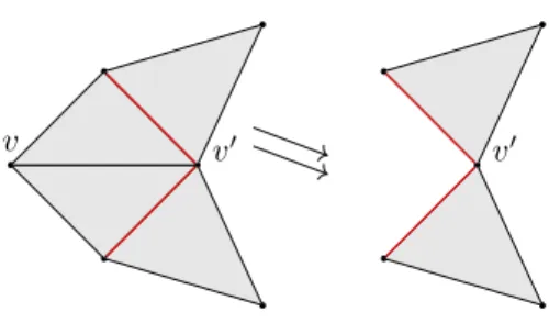
Figure 1 Illustration of an elementary strong collapse. In the complex on the left, v is dominated
by vÕ. The link of v is highlighted inred. Removing v leads to the complex on the right.
Strong collapse: An elementary strong collapse is the deletion of a dominated vertex
v from K, which we denote with K √√e K\ v. Figure 1 illustrates an easy case of an elementary strong collapse. There is a strong collapse from a simplicial complex K to its subcomplex L, if there exists a series of elementary strong collapses from K to L, denoted as
K √√ L. The inverse of a strong collapse is called a strong expansion. If there exists a combination of strong collapses and/or strong expansion from K to L then K and L are said to have the same strong homotopy type.
The notion of strong homotopy type is stronger than the notion of simple homotopy type in the sense that if K and L have the same strong homotopy type, then they have the same simple homotopy type, and therefore the same homotopy type [1]. There are examples of contractible or simply collapsible simplicial complexes that are not strong collapsible.
A complex without any dominated vertex will be called a minimal complex. A core of a complex K is a minimal subcomplex Kc
™ K, such that K √√ Kc. Every simplicial
complex has a unique core up to isomorphism. The core decides the strong homotopy type of the complex, and two simplicial complexes have the same strong homotopy type iff they
have isomorphic cores [1, Theorem 2.11].
Retraction map: If vÕ dominates v in K. The vertex map r : K æ K \ v defined as:
r(w) = w if w ”= v and r(v) = vÕ, induces a simplical map that is a retraction map. The
homotopy between r and the identity over K \ v is in fact a strong deformation retract.
Nerve of a simplicial complex: An open cover U of a topological space X is a set of open sets of X , such that X is a subset of their union. The nerve of a cover U is an abstract simplicial complex, defined as the set of all non-empty intersections of the elements of U. The nerve is a well known construction that transforms a continuous space to a combinatorial space preserving its homotopy type. The nerve N (K) of a simplicial complex K is defined as the nerve of the set of maximal simplices of the complex K (considered as a cover of the complex). Hence all the maximal simplices of K will be the vertices of N (K) and their non-empty intersection will form the simplices of N (K). For j Ø 2 the iterative construction is defined as Nj(K) = N (Nj≠1(K)). This definition of nerve preserves the homotopy type,
Kƒ N (K)[1]. A remarkable property of this nerve construction is its connection with strong collapses.
Taking the nerve of any simplicial complex K twice corresponds to a strong collapse. We will state it as a theorem below and recall the proof from [1] in the Appendix.
ITheorem 1. [1, Proposition 3.4] For a simplicial complex K, there exists a subcomplex L isomorphic to N2(K), such that K√√L.
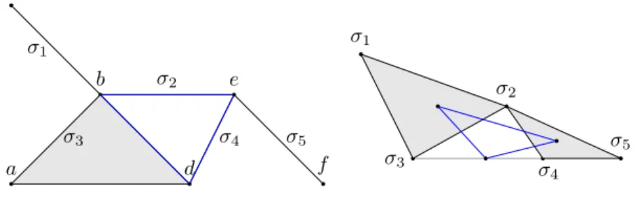
a b c d e f ‡3 ‡1 ‡2 ‡4 ‡5 ‡3 ‡1 ‡2 ‡4 ‡5
Figure 2 Left: K (in grey), Right: N (K) (in grey) and N2(K) (inblue). N2(K) is isomorphic
to a full-subcomplex of K highlighted inblueon the left.
An easy consequence of this theorem is that a complex K is minimal if and only if it is isomorphic to N2(K) [1, Lemma 3.6]. This means that we can keep collapsing our
complex K by applying N2(≠) iteratively until we reach the core of the complex K. The
se-quence K, N2(K), ..., N2p(K) is a decreasing sequence up to isomorphism. It leads to the easy
however deep consequence that K is strong collapsible iff N2p(K) is a point for some p Ø 1 [1].
3
Algorithm
In this section, we describe an algorithm to strong collapse a simplicial complex K, provide the details of the implementation and analyze its complexity. We construct N2(K) as defined
in Section 2.
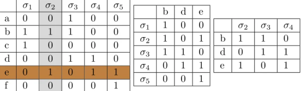
Data structure: Basically, we represent K as the adjacency matrix M between the vertices
and the maximal simplices of K. We will simply call M the adjacency matrix of K. The rows of M represent the vertices and the columns represent the maximal simplices of K. For convenience, we will identify a row (resp. column) and the vertex (resp. maximal simplex) it represents. An entry M[vi][‡j] associated to a vertex vi and a maximal simplex
‡j is set to 1 if vi œ ‡j, and to 0 otherwise. For example, the matrix M in the left of the
Table 1 corresponds to the leftmost simplicial complex K in Figure 2. Usually, M is very sparse. Indeed, each column contains at most d + 1 non-zero element since the simplices of a
d-dimensional complex have at most d+1 vertices, and each line contains at most 0non-zero
elements where 0 is an upper bound on the number of maximal simplices incident to a
given vertex. In most practical situations, 0 is a small fraction of the number of maximal
simplices [31, Table 5]. It is therefore beneficial to store M as a list of vertices, each vertex giving access to a list of maximal simplices that contain the vertex, and a list of maximal simplices, each simplex giving access to its list of vertices. This is similar to the SAL data structure of [31].
Core algorithm: Given the adjacency matrix M of K, we compute the adjacency matrix C
of the core Kc. It turns out that using basic row and column removal operations, we can
easily compute C from M. Loosely speaking our algorithm recursively computes N2(K)
until it reaches Kc.
The columns of M (which represent the maximal simplices of K) correspond to the vertices of N (K). Also, the columns of M that have a non-zero value in a particular row
‡
1‡
2‡
3‡
4‡
5a 0
0
1
0
0
b 1
1
1
0
0
c
1
0
0
0
0
d 0
0
1
1
0
e
0
1
0
1
1
f
0
0
0
0
1
b d e
‡
11 0 0
‡
21 0 1
‡
31 1 0
‡
40 1 1
‡
50 0 1
‡
2‡
3‡
4b 1
1
0
d 0
1
1
e
1
0
1
Table 1 From left to right M, N (M) and N2(M)
Therefore, each row of M represents a simplex of the nerve N (K). Not all the simplices of N (K) are associated to rows of M but all maximal simplices are since they correspond to subsets of maximal simplices with a common vertex. To remedy this situation, we remove all the rows of M that correspond to non-maximal simplices of N (K). This results in a new smaller matrix M whose transpose, noted N (M), is the adjacency matrix of the nerve N (K). We then exchange the roles of rows and columns (which is the same as taking the transpose) and run the very same procedure as before so as to obtain the adjacency matrix N2(M) of
N2(K).
The process is iterated as long as the matrix can be reduced. Upon termination, we output the reduced matrix C := N2p(M), for some p Ø 1, which is the adjacency matrix of
the core Kc of K. Removing a row or column is the most basic operation of our algorithm.
We will discuss it in more detail later in the paragraph Domination test.
Example: As mentioned before, the matrix M in the left of the Table 1 represents the
simplicial complex K in the left of Figure 2. We go through the rows first, rows a and c are subsets of row b and row f is a subset of e. Removing rows a, c and f and transposing it, yields the adjacency matrix N (M) of N (K) in the middle. Now, row ‡1 is a subset of
‡2 and of ‡3, also ‡5is a subset of ‡2 and of ‡4. We remove these two rows of N (M) and
transpose it and get the rightmost matrix N2(M), which corresponds to the core drawn in
blue in Figure 2.
Domination test: Now we explain in more detail how to detect the rows that need to be removed. Let v be a row of M and ‡v be the associated simplex in N (K). If ‡v is
not a maximal simplex of N (K), it is a proper face of some maximal simplex ‡vÕ of N (K).
Equivalently, the row vÕ of M that is associated to ‡
vÕ contains row v in the sense that the
non zero elements of v appear in the same columns as the non zero elements of vÕ. We will
say that row v is dominated by row vÕ and determining if a row is dominated by another
one will be called the row domination test. Notice that when a row v is dominated by a row
vÕ, the same is true for the associated vertices since all the maximal simplices that contain
vertex v also contain vertex vÕ, which is the criterion to determine if v is dominated by vÕ
(See Remark 1 in Section 2). The algorithm removes all dominated rows and therefore all dominated vertices of K.
After removing rows, the algorithm removes the columns that are no longer maximal in
K, which might happen since we removed some rows. Removing a column may lead in turn
to new dominated vertices and therefore new rows to be removed. When the algorithms stops, there are no rows to be removed and we have obtained the core Kc of the complex K.
The algorithm in fact provides a constructive proof of Theorem 1.
Removing columns is done in very much the same way: we just exchange the roles of rows and columns.
Computing the retraction map r: The algorithm also provides a direct way to compute
the retraction map r defined in Section 2. The retraction map corresponding to the strong collapses executed by the algorithm can be constructed as follows. A row being removed in
M corresponds to a dominated vertex in K and the row which contains it corresponds to a
dominating vertex. Therefore we map the dominated vertex to the dominating vertex and compose all such maps to get to the final retraction map from K to its core Kc. The final
map is simplicial as well as it is a composition of simplicial maps.
Reducing the number of domination tests: We first observe that, when one wants to
determine if a row v is dominated by some other row, we don’t need to test v with all other rows but with at most d of them. Indeed, at most d + 1 rows can intersect a given column since a simplex can have at most d + 1 vertices. For example, in Table 1 (Left), to check if row e (highlighted inbrown) is dominated by another row, we pick the first non-zero column
‡2(highlighted in Gray) and compare e with the non-zero entries {b} of ‡2.
A second observation is that we don’t need to test all rows and columns for domination, but only the so-called candidate rows and columns. We define a row to be a candidate
row for the next iteration if at least one column containing one of its non-zero elements has
been removed in the previous column removal iteration. Similarly, by exchanging the roles of rows and columns, we define the candidate columns. Candidate rows and columns are the only rows or columns that need to be considered in the domination tests of the algorithm. Indeed, a column · of M whose non-zero elements all belong to rows that are present from the previous iteration cannot be dominated by another column ·Õ of M, since · was not
dominated at the previous iteration and no new non-zero elements have been added. The same argument follows for the candidate rows.
We maintain two queues, one for the candidate columns (colQueue) and one for the candidate rows (rowQueue). These queues are implemented as First in First out (FIFO) queues. At each iteration, we pop out a candidate row or column from its respective queue and test whether it is dominated or not. After each successful domination test, we push the candidate columns or rows in their appropriate queue in preparation for the subsequent iteration. In the first iteration, we push all the rows in rowQueue and then alternatively use colQueue and rowQueue. Algorithm 1 gives the pseudo code of our algorithm.
Time Complexity: The most basic operation in our algorithm is to determine if a row is a dominated by another given row, and similarly for columns. In our implementation, the rows (columns) of the matrix that are considered by the algorithm are stored as sorted lists. Checking if one sorted list is a subset of another sorted list can be done in time O(l), where l is the size of the longer list. Note that the length of a row list is at most 0where 0denotes
an upper bound on the number of maximal simplices incident to a vertex. The length of a column list is at most d + 1 where d is the dimension of the complex. Hence checking if a row is dominated by another row takes O( 0) time and checking if a column is dominated
by another column takes O(d) time.
At each iteration on the rows (Lines 7-13 of Algorithm 1), each row is checked against at most d other rows (since a maximal simplex has at most d + 1 vertices), and at each iteration of the columns (Lines 18-24 of Algorithm 1), each column is checked against at most 0
Algorithm 1 Core algorithm
1: procedure Core(M) Û Returns the matrix corresponding to the core of K
2: rowQueueΩ push all rows of M (all vertices of K)
3: colQueueΩ empty
4: while rowQueue is not empty do
5: vΩ pop(rowQueue)
6: ‡Ω the first non-zero column of v
7: for non-zero rows w in ‡ do
8: if v is a subset of w then
9: Remove v from M
10: push all non-zero columns · of v to colQueue if not pushed before
11: break
12: end if
13: end for
14: end while
15: while colQueue is not empty do
16: ·Ω pop(colQueue)
17: vΩ the first non-zero row of ·
18: for non-zero columns ‡ in v do 19: if · is subset of ‡ then
20: Remove · from M
21: push all non-zero rows w of · to rowQueue if not pushed before
22: break
23: end if 24: end for
25: end while
26: if rowQueue is not empty then
27: GOTO 4
28: end if
29: return M ÛThe core consists of the remaining rows and columns
other columns (since a vertex can belong to at most 0maximal simplices). Since, at each
iteration on the rows, we remove at least one row, the total number of iterations on the rows is at most O(v2), where v is the total number of vertices of the complex K. Similarly,
at each iteration on the columns, we remove at least one column and the total number of iterations on columns is O(m2), where m is the total number of maximal simplices of the
complex K. The worst-case time complexity of our algorithm is therefore O(v2 0d+ m2 0d).
Observe that m is exponentially smaller (wrt d) than the total number of simplices. Moreover
0Æ m/n and is usually a small fraction of the number of maximal simplices [31].
4
Strong collapse of zigzag sequences
In this section, we begin with some brief background on quiver theory and zigzag persistence, enough to present our main result. Readers interested in more details can refer to [22, 23, 26].
Quivers: A quiver Q is a directed graph, more formally it’s a pair of sets (Q0, Q1),
where Q0= {v1, v2, ...vn}; n œ N is the set of vertices and Q1 is the set of directed edges
between the vertices. Given a field F, an F-representation V = (Vi, fij) of a quiver Q
is an assignment of a finite dimensional F-vector spaces Vi for every vertex vi œ Q0 and
a homomorphism fij : Vi æ Vj for each directed edge eij œ Q1. A morphism „ between
two different F-representations V = (Vi, fij) and W = (Wi, gij) of a quiver Q is a set of
homomorphisms „i : Vi æ Wi such that, for every edge eij œ Q1, „jfij = gij„i. In other
words all the squares in two representations connected by „is commute. A morphism „ is
an isomorphism (≥=) if all individual „is are bijective. A direct sum V ü W between two
different F-representations is defined using the direct sum of the individual vector spaces
Viü Wi at each vertex vi and direct sum (component-wise application) homomorphisms
fijü gij for each edge eij. An F-representation V is decomposable if it is isomorphic to
a direct sum of two non-trivial F-representations. Otherwise it is called indecomposable. These indecomposable F-representations of a quiver can be thought of as building blocks of the decomposable representations.
Zigzag module: A zigzag module is a "topological" representation of a quiver whose
underlying graph is a Dynkin graph of type An. Here the vector spaces are (co)homology
classes with induced homomorphisms between them. If a quiver Q is of type An, for two
integers b and d, 0 Æ b Æ d Æ n; we can define an interval F-representation I[b, d] of Q by assigning the vector space F for each vi when i œ [b, d], and null spaces otherwise, the
maps between any two F vector space is identity and is zero otherwise. These intervals representations are precisely the indecomposable representations for quivers of type An.
A result by Gabriel [22, Theorem 11] says that every F-representation V of a quiver of type An can be decomposed as the direct sum of finitely many interval representations. In
particular this means that a zigzag module can be represented with a finite set of intervals. These intervals pertain topological information as they indicate birth and death of homology classes. The multiset of all the intervals [bj, dj] is called a zigzag (persistence) diagram.
The zigzag diagram completely characterizes the zigzag module, that is, there is bijective correspondence between them [22, 18].
Given a zigzag sequence of simplicial complexes Z : {K1≠æ Kf1 2Ω≠ Kg2 3≠æ · · ·f3 ≠≠≠≠æf(n≠1)
Kn}, the most common way to get a zigzag module is to compute homology classes of these
sequences with field coefficients. The zigzag module of Z, P(Z) : {Hp(K1) f1ú
≠æ Hp(K2) gú2
Hp(K3) f3ú
≠æ · · · f
ú (n≠1)
≠≠≠≠æ Hp(Kn)}. Here p is the dimension of the homology class and ú
denotes the induced homomorphisms. A zigzag sequence is called a simplicial tower if all maps are forward. i.e. only fis. A tower is called filtration if the maps are only inclusions.
A zigzag module arising from a sequence of simplicial complexes captures the evolution of the topology of the sequence, encoded it in its zigzag (persistence) diagram.
Strong collapse of the zigzag module: Given a zigzag sequence Z : {K1 ≠æ Kf1 2 Ω≠g2
K3 ≠æ · · ·f3 ≠≠≠≠æ Kf(n≠1) n}. We define the core sequence Zc of Z as Zc : {K1c fc 1 ≠æ Kc 2 gc 2 Ω≠ Kc 3 fc 3 ≠æ · · · f c (n≠1) ≠≠≠≠æ Kc
n}. Where Kic is the core of Ki. The forward maps are defined as,
fc
j := rj+1fjij; and the backward maps are defined as gcj := rjgjij+1. The maps ij : KjcÒæ Kj
and rj : Kjæ Kjc are the composed inclusions and the retractions maps defined in Section
2 respectively.
ITheorem 2. Zigzag modules P(Z) and P(Zc) are equivalent.
Proof. Consider the following diagram
K1 K2 K3 · · · Kn≠1 Kn Kc 1 K2c K3c · · · Knc≠1 Knc f1 r1 r2 g2 r3 fn≠1 rn≠1 rn fc 1 g2c fn≠1c
and the associated diagram after computing the p-th homology groups
Hp(K1) Hp(K2) Hp(K3) · · · Hp(Kn≠1) Hp(Kn) Hp(K1c) Hp(K2c) Hp(K3c) · · · Hp(Knc≠1) Hp(Knc) f1ú rú1 rú2 gú2 r3ú fnú≠1 rú n≠1 rún (fc 1)ú (gc 2)ú (fc n≠1)ú
ú represents the induced homomorphisms between the homology classes by the corresponding simplicial maps. Since there exists a strong deformation retract between rj and ij, the
induced homomorphisms rú
j and iúj are isomorphisms [29, Corollary 2.11]. Also, (fjc)ú =
(rj+1fjij)ú = rúj+1fjúiúj = fjú and similarly (gjc)ú = gúj, see [29, Proposition (1) page 111].
Therefore all the squares in the lower diagram commute. Now the top and bottom rows are two different representations of the same underlying quiver. The set of maps rú
js are bijective
(isomorphisms on the vector spaces), therefore these two representations are isomorphic and
hence their zigzag diagrams are identical. J
In fact, using the notion of quiver representation this result follows for the multidimensional persistence as well.
5
Computational experiments
For each data set, we consider as the input sequence a nested sequence (filtration) of Vietoris-Rips (VR) complexes associated to a set of increasing values of the scale parameter (called snapshots). We first independently strong collapse all these complexes, then assemble the resulting individual cores using the induced simplicial maps introduced in Section 4. The resulting new sequence with induced simplicial maps between the collapsed complexes is usually a simplicial tower. We then convert the simplicial tower into an equivalent filtration using the software Sophia [38] that implements an algorithm of Dey et. al. [20]. Finally, we
X
1-sphere 2-Annulus dragon netw-sc senate eleg
Snp
80
80
46
69
107
77
Flt(10
6)
0.12
13.91
7.96
22.35
2.56
1.18
Twr
54
252
1,641
380
104
298
EqF
573
1,954
8,437
957
270
431
Flt/EqF(10
3) 0.21
7.12
0.94
23.35
9.48
2.74
0.65
174.18
69.92
243.86
24.92
10.87
MCT
0.005
0.022
0.065
0.009
0.003
0.002
AT
0.045
0.136
0.408
0.078
0.06
0.157
PDT
0.01
0.02
0.08
0.01
0.005
0.006
Total
0.060
0.178
0.553
0.097
0.068
0.165
PDF/Total
10.8
978.5
126.4
2514.0
366.5
65.9
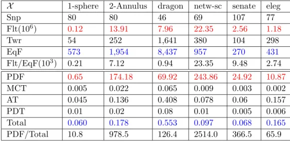
Table 2 The rows are, from top to down: dataset X , number of snapshots (snp), total number
of simplices in the original filtration (Flt), number of simplices in the collapsed tower (Twr), total number of simplices in the equivalent filtration (EqF), ratio of Flt and EqF (Flt/EqF), PD computation time for the original filration (PDF), maximum collapse time (MCT), assembly time (AT), PD computation time of the tower (PDT), sum MCT+AT+PDT (Total), ratio of PDF and Total (PDF/Total). All times are noted in seconds. For the first three datasets, we sampled points randomly from the initial datasets and averaged the results over five trials.
run the persistence algorithm of the Gudhi library [37] to obtain the persistence diagram (PD) of the equivalent filtration. By the results of Section 4, the obtained PD is the same as
the PD of the initial sequence.
The total time to compute the PD of the core sequence is the sum of three terms: 1. the
maximum time taken to collapse all the individual complexes, 2. the time taken to assemble
the individual cores to form a tower, 3. the time to compute the persistent diagram of the tower. Table 2 summarises the results of the experiments. In both cases, the original filtration and the collapsed tower, we use Gudhi through Sophia which is done through the command <./sophia -cgudhi inputTowerFile outputPDFile>. When we use the -cgudhi option, Sophia reports two computation times, one the total time taken by Sophia that includes (1) reading the tower, (2) transforming it to a filtration and (3) time taken by Gudhi to compute PD, second reported time is just the time taken by Gudhi to compute PD. In our comparison, for the original filtration we report just the Gudhi time and for the collapsed tower we report the total time taken by Sophia.
The dataset of the first column (1-sphere) of Table 2 consists of 100 random points sampled from a unit circle in dimension 2. The dataset of the second column (2-Annulus) consists of 150 random points sampled from a two dimension annulus of radii {0.6, 1}. For all the other experiments, we use datasets from a publicly available repository [43]. These datasets have been previously used to benchmark different publicly available software computing PH [42]. For the third experiment (dragon), we randomly picked 150 points from the 2000 points of the dataset drag 2 of [43]. The fourth and fifth column respectively correspond to the dataset netw-sc and senate of [43], here we used the distance matrix. The sixth column corresponds to the dataset eleg of [43], and here again we used the distance matrix. The first three datasets are point sets in Euclidean space. For the other three, the distance matrices of the datasets were available at [43]. The [initial value, increment, final value] of the scale
dimension snapshot = all fitration values?
parameter are [0.1, 0.005, 0.5], [0.1, 0.005, 0.5], [0, 0.001, 0.046], [0.1, 0.05, 3.5], [0, 0.001, 0.107] and [0, 0.001, 0.077] for the examples in Table 2 (from left to right). For more detail about the datasets and the computation of the distance matrices of the last three datasets please refer to [42].
The plots below count the maximal simplices and the dimensions of the complexes across the filtration and the collapsed tower. Blueandredcorrespond respectively to the filtration and the collapsed tower of the data netw-sc. Similarlygreenandbrowncorrespond respectively to the filtration and the collapsed tower of the data senate. Finally, black and
cyancorrespond to the filtration and the collapsed tower of the data eleg respectively. We can observe that in all cases the number of maximal simplices either stays near constant or decreases. Also they are far fewer in number compared to the total number of simplices. Observe that for the uncollapsed filtrations blue, greenand black, the dimension of the complexes increases quite rapidly with the snapshot index. Although dimensions are small, their effect on the total number of simplices is exponential. Another key fact to observe is that the dimension of the complexes in the corresponding collapsed tower are much smaller than their counterparts in the filtration.
0 15 30 45 60 75 90 105 0 50 100 150 200 250 300 350 400 Snapshot index Nu m of M ax im al Si m pl ic es
Count of maximal simplices across filtrations
0 15 30 45 60 75 90 105 0 2 4 8 12 16 20 Snapshot index D im en si on of th e com pl ex
Dimension of the complex across filtrations
Noticeably, in our experiments, the computing time of our approach is reduced by 1 to 3 orders of magnitude. The gain is more with the size of the filtration. A similar reduction of 2 to 4 orders of magnitude is achieved for the number of simplices. Observations from the plots combined with the experimental results of Table 2 clearly indicate that our method is extremely fast and memory efficient.
The implementation of the Core algorithm 1 bench-marked here is coded in C++ and will be available as an open-source package of the next release of the Gudhi library [37]. The code was compiled using the compiler <clang-900.0.38> and all computations were performed on <2.8 GHz Intel Core i5> machine with 16 GB of available RAM.
The experiments above are limited to filtrations of VR-complexes, by far the most commonly used type of sequences in Topological Data Analysis. We intend to experiment on Zigzag sequences in future work.
Acknowledgements. We want to thank Marc Glisse for his useful discussions, Mathijs
Wintraecken for reviewing a draft of the article. We also want to thank Francois Godi and Siargey Kachanovich for their help with Gudhi and Hannah Schreiber for her help with Sophia.
References
1 J.A. Barmak, E.G. Minian. Strong homotopy types, nerves and collapses. Discrete and Computational Geometry 47(2012), pp. 301-328.
2 M. Tancer: Recognition of collapsible complexes is NP-complete. Discrete and Computa-tional Geometry. 55(1) (2016), 21-38.
3 D. Attali, A. Lieutier, and D. Salinas. Efficient data structure for representing and sim-plifying simplicial complexes in high dimensions. International Journal of Computational Geometry and Applications (IJCGA), 22(4):279–303, 2012.
4 A. C. Wilkerson, T. J. Moore, A. Swami,and A. H. Krim. Simplifying the homology of networks via strong collapses. ICASSP - Proceedings (2013).
5 A. C. Wilkerson, H. Chintakunta and H. Krim. Computing persistent features in big data: A distributed dimension reduction approach. ICASSP - Proceedings (2014) pp. 11-15.. 6 C. H. Dowker, “Homology groups of relations,” The Annals of Mathematics, vol. 56, pp.
84–95, 1952.
7 M. Adamaszek and J. Stacho. Complexity of simplicial homology and independence com-plexes of chordal graphs. Computational Geometry: Theory and Applications. 57, 8–18 (2016).
8 K. Mischaikow and V. Nanda. "Morse Theory for Filtrations and Efficient Computation of Persistent Homology". DCG, Volume 50, Issue 2, pp 330-353, September 2013.
9 Michael Kerber and R. Sharathkumar. “Approximate ech Complex in Low and High Dimensions”. In: Algorithms and Computation. Ed. by Leizhen Cai, Siu-Wing Cheng, and Tak-Wah Lam. Vol. 8283. Lecture Notes in Computer Science. 2013, pp. 666–676.
10 Donald Sheehy.“Linear-Size Approximations to the Vietoris–Rips Filtration”. In: Discrete and Computational Geometry 49.4 (2013), pp.778–796.
11 Afra Zomorodian. “The Tidy Set: A Minimal Simplicial Set for Computing Homology of Clique Complexes”. In: Proceedings of the Twenty-sixth Annual Symposium on Compu-tational Geometry. SoCG’10. Snowbird, Utah, USA, 2010, pp. 257–266. isbn: 978-1-4503-0016-2.
12 M. Botnan. and G Spreemann. "Approximating persistent homology in Euclidean space through collapses". In: Applicable Algebra in Engineering, Communication and Computing 26 (1-2), 73-101.
13 P. D≥otko, H. Wagner, Simplification of complexes for persistent homology computations, Homology, Homotopy and Applications, vol. 16(1), 2014, pp.49 - 63.
14 T. K. Dey, H. Edelsbrunner, S. Guha and D. Nekhayev. Topology preserving edge contrac-tion. . Publications de l’Institut Mathematique (Beograd), Vol. 60 (80), 23–45, 1999. 15 C. Chen and M. Kerber. Persistent homology computation with a twist. In European
Workshop on Computational Geometry (EuroCG), pages 197-200, 2011.
16 U. Bauer, M. Kerber, and J. Reininghaus. Clear and compress: Computing persistent homology in chunks. In Topological Methods in Data Analysis and Visualization III, Math-ematics and Visualization, pages 103-117. Springer, 2014.
17 François Le Gall. Powers of tensors and fast matrix multiplication. ISSAC ’14, pages 296–303. ACM, 2014.
18 A. Zomorodian and G. Carlsson. Computing persistent homology. Discrete Comput. Geom., 33(2):249–274, 2005.
19 H. Edelsbrunner, D. Letscher, and A. Zomorodian. Topological persistence and simplifica-tion. Discrete Comput. Geom., 28:511–533, 2002.
20 T. Dey, F. Fan, and Y. Wang. Computing Topological Persistence for Simplicial Maps. In ACM Symposium on Computational Geometry (SoCG), pages 345-354, 2014.
21 F. Chazal, S. Oudot. Towards Persistence-Based Reconstruction in Euclidean Spaces. In Proc. ACM Symp. of Computational Geometry 2008.
22 Gunnar Carlsson and Vin de Silva. "Zigzag Persistence". Found Comput Math (2010) 10: 367.
23 Gunnar Carlsson, Vin de Silva, and Dmitriy Morozov. Zigzag persistent homology and real-valued functions. SOCG (2009), pages 247-256.
24 C. Maria and S. Oudot. “Zigzag Persistence via Reflections and Transpositions”. In: Proc. ACM-SIAM Symposium on Discrete Algorithms (SODA). Jan. 2015, pp. 181–199.
25 Nikola Milosavljevic, Dmitriy Morozov, and Primoz Skraba. Zigzag persistent homology in matrix multiplication time. In Symposium on Comp. Geom., 2011.
26 Harm Derksen and Jerzy Weyman. Quiver representations. Notices of the American Math-ematical Society, 52(2):200–206, February 2005.
27 Cohen-Steiner, David; Edelsbrunner, Herbert and Harer,John. Stability of Persistence Dia-grams. Discrete Comput. Geom., 37(1):103-120, 2007.
28 Herbert Edelsbrunner and John Harer. Computational Topology: An Introduction. Amer-ican Mathematical Society, 2010.
29 A. Hatcher. Algebraic Topology. Cambridge Univ. Press, 2001.
30 J.H.C Whitehead. Simplicial spaces, nuclei and m-groups. Proc. London Math. Soc. 45 (1939), 243-327.
31 Jean-Daniel Boissonnat, Karthik C. S., Sébastien Tavenas: Building Efficient and Compact Data Structures for Simplicial Complexes. Algorithmica 79(2): 530-567 (2017).
32 Jean-Daniel Boissonnat, Karthik C. S.: An Efficient Representation for Filtrations of Sim-plicial Complexes. ACM-SIAM Symposium on Discrete Algorithms (SODA 2017).
33 Gunnar Carlsson, Tigran Ishkhanov, Vin de Silva, and Afra Zomorodian. “On the Local Behavior of Spaces of Natural Images”. In: International Journal of Computer Vision 76.1 (2008), pp. 1–12.
34 Joseph Minhow Chan, Gunnar Carlsson, and Raul Rabadan. “Topology of viral evolution”. In: Proceedings of the National Academy of Sciences 110.46 (2013), pp. 18566–18571. 35 Vin de Silva and Robert Ghrist. “Coverage in sensor networks via persistent homology”. In:
Algebraic and Geometric Topology 7 (2007), pp. 339 – 358.
36 Jose Perea and Gunnar Carlsson. “A Klein-Bottle-Based Dictionary for Texture Represent-ation”. In: International Journal of Computer Vision 107.1 (2014), pp. 75–97.
37 Gudhi: Geometry understanding in Higher Dimensions. http://gudhi.gforge.inria.fr/ 38 Sophia: https://bitbucket.org/schreiberh/sophia/
39 Phat: https://bitbucket.org/phat-code/phat 40 Ripser: https://github.com/Ripser/ripser
41 Dionysus: http://www.mrzv.org/software/dionysus/
42 N. Otter, M. Porter, U. Tillmann, P. Grindrod and H. Harrington. "A roadmap for the computation of persistent homology", EPJ Data Science 2017 6:17, Springer Nature. 43 Datasets: "https://github.com/n-otter/PH-roadmap/"
6
Appendix
Proof of Theorem 1 : We recall the following crucial lemma from [1, Lemma 3.3], required to prove the Theorem 1 .
ILemma 3. Let L be a full subcomplex of a simplicial complex K, such that every vertex vœ K, /œ L is dominated by some vertex in L, then K√√L.
The vertices of N2(K) are the maximal family of the maximal simplices of K that has
a common intersection. That is, if s= {‡0s, ‡1s, ..., ‡sis} is a vertex of N
maximal set such that u
0ÆjÆis ‡s
j ”= ÿ, where the ‡sjsare maximal simplices of K. A 1≠simplex
of N2(K) is a pair
sand tsuch that sfl t”= ÿ and sfl tis a set of maximal simplices
of K. Otherwise sfi t would be a maximal family of intersecting maximal simplices,
contradicting the maximality of s and t. Similarly, all the higher dimensional simplices
will follows this condition of existence.
Now we define a map „ : N2(K) æ K, such that, if
s is a vertex of N2(K) then
„( s) œ u
0ÆjÆis ‡s
j. We claim that „ is injective, simplicial and its image is a full subcomplex
of K.
„is injective: Let 0and 1be two vertices of N2(K), such that „( 0) = „( 1) = v œ K.
Then v œ u
0ÆjÆi0
‡0j and v œ
u
0ÆjÆi1
‡1j, which implies v is a common vertex in the maximal
simplices which defines both 0 and 1. Therefore 0fi 1 is a family of interesecting
maximal simplices of K. Since 0and 1 are maximal, 0= 1= 0fi 1.
„is simplicial: Let [ 0, 1, ..., k] be a k-simplex of N2(K), then there exists a maximal
simplex ‡ of K, such that, ‡ œ s,’s = 0...k. By definition of „, „( s) œ ‡ for all s.
Therefore „([ 0, 1, ..., k]) spans a face of ‡, which is a simplex in K.
„(N2(K)) is a full subcomplex of K : Let ‡ be a simplex of K spanned by {„( 0), „( 1), ..., „( r)}
and let ‡Õ
is a maximal simplex of K, such that ‡ ™ ‡Õ
. Since „( s) œ ‡ ™ ‡
Õ
,
‡Õœ s,’s = 0...r, hence { 0, 1, ..., r} spans a simplex in N2(K).
The existence of such a map „ proves the following lemma.
ILemma 4. N2(K) is isomorphic to a full subcomplex of K.
Let v be a vertex of K, which is not in the image „(N2(K)). Let = {‡
0, ‡1, ..., ‡l} be
the set of all the maximal simplices of K that contains v. Since v is not in the image of „, may or may not be maximal. Hence there exists a vertex s of N2(K), such that, ™ s.
By definition „( s) dominates v. Therefore „(N2(K)) satisfies the hypothesis of Lemma 6,