Characterization of a series viscous actuator for use in rehabilitative robotics

Characterization of a Series Viscous Actuator For

Use in Rehabilitative Robotics

by

Nicholas Eric Wiltsie

Submitted to the Department of Mechanical Engineering

OF TECHNOLOcjY

Bachelor of Science in Mechanical Engineering

at the

JUN

3 0 2010

MASSACHUSETTS INSTITUTE OF TECHNOLOGY

LIBRARIES

June 2010

©

Massachusetts Institute of Technology 2010. All rights reserved.

Author ...

Department of Mechanical Engineering

May 10, 2010

Certified by...

Neville Hogan

Professor of Mechanical Engineering

Thesis Supervisor

Accepted by ...

C'oillis rofessor of

ohn H. Lienhard V

Mechanical Engineering

Chairman, Undergraduate Thesis Committee

Characterization of a Series Viscous Actuator For Use in

Rehabilitative Robotics

by

Nicholas Eric Wiltsie

Submitted to the Department of Mechanical Engineering on May 10, 2010, in partial fulfillment of the

requirements for the degree of

Bachelor of Science in Mechanical Engineering

Abstract

In this thesis, a series viscous actuator, composed of a viscous rotary damper con-nected to the output of a geared electric motor, is proposed as a novel solution to the high actuator impedances encountered when using such a motor. High impedances can be undesirable when interacting with the environment or animal subjects as un-expected forces may damage already-compromised joints. A state space model for the series viscous actuator was derived and verified by measurements upon a physical sys-tem. Physical design considerations for implementing a series viscous actuator, such as the appropriate gearing ratio and damper selection, are discussed and supported using the derived model.

Thesis Supervisor: Neville Hogan

Acknowledgments

The author would like to thank Yun-Seong Song and Neville Hogan for their invaluable help in completing this project.

Contents

1 Introduction . . . . 8

2 Background . . . . 8

2.1 SVA State Equations . . . . 8

2.2 System Dynamics . . . . 12

2.3 SVA Impedance . . . . 13

3 Experimental Design . . . . 14

3.1 SVA Design . . . . 14

3.2 Damper Characterization . . . . 14

3.3 System Dynamics Verification . . . . 15

3.4 SVA Impedance Measurement . . . . 16

4 Results . . . . 17

4.1 SVA Design . . . . 17

4.2 Damper Characterization . . . . 18

4.3 System Verification . . . . 19

4.4 SVA Impedance Measurement . . . . 20

5 Discussion . . . . 22

1

Introduction

The need for low-impedance actuators when interacting with humans or animals has recently been emerging. Particularly in the field of rehabilitative robotics, a high output-impedance actuator can be dangerous if it interferes with the subject's natural movement; due to inadequate muscle tone, a joint such as the shoulder may be particularly vulnerable to unexpected resistance. However, most actuators with high enough torque output usually suffer from high output impedance. For example, the gearbox necessary to transform the high-speed low-torque output of an ordinary

DC motor into a low-speed high-torque output increases the motor inertia as the

square of the gear ratio, in addition to introducing significant friction. These sum to a high-impedance output that is difficult to back-drive.

Previous work on this problem has resulted in the development of series elastic actuators (SEA) consisting of an elastic spring in series with the high-impedance actuator. In exchange for altered dynamics and increased complexity, the output force is delivered through the low-impedance spring. However, SEAs have limited travel and displacement-dependent impedance. As an alternative, series viscous actuators (SVA) have been proposed. Previous work on this project has resulted in an experimental setup consisting of a brushed DC motor in series with a gearbox and a viscous damper, with the far end of the damper connecting to a static torque gauge. A computer with data acquisition setup commands the motor, reads and logs the outcome. This system was characterized using linear models, and the expected torque outputs resulting from ramp and step voltage inputs were compared with measured results on the physical system.

2

Background

2.1

SVA State Equations

The physical SVA system is designed as shown in Figure (1), and the equivalent impedance model is shown in Figure (2); it consists of a DC motor in series with a

SVA

Vin

Motor Gearbox B1 B2

Figure 1: System diagram of a loaded SVA

SVA Motor

R L 0

Gearbox

Figure 2: Equivalent impedance diagram of a loaded SVA

gearbox connects to a load through a rotary damper, B1. The motor is modeled as a resistance R in series with an electrical-to-mechanical transformer. The motor and gearbox have rotary inertias Jm and Jg, respectively. The load is modeled as a rotary intertia J in series with a second rotary damper, B2, fixed to the ground.

The derivation of the system model begins with the constitutive equations

r. = KT -1 ₍₁₎

Vemf = KT w, (2)

ET = Jo (3)

T = B(Aw) (4)

Equations (1) and (2) relate the electrical inputs of the motor to the mechanical outputs through the motor constant KT, while (3) and (4) are the characteristic equations of a rotating mass and a rotary damper.

the two state variables of the system, with the input voltage Vm as the driving input. The state equations are obtained via manipulations of the free body diagrams of the following subsystems:

TI --- O-X -NT

WBia

Figure 3: Subsystems of loaded SVA

The first state equation is the torque balance of the fourth subsystem,

(5) JLL 2 = -B22- B1(w2 - W1)

The other state equation requires the inclusion of the motor dynamics,

Vn = Vemf + RI = KTwm + RTm

Kt (6)

as well as the relationship between the internal variables on either side of the gearbox, T2 ~ ₁

Wm W1 = 9W2

elim-inating the internal variables Ti, T2, Tm, and Wm reveals the final state equation: Tm - ri = JmAJm T2 Tm- -- = Jmgw1 9 72 = grm - Jm92C)i T2- B1(wi - w₂) = Jdi T2 = Jgu)1 + B1(wi - w₂) g7m - Jmg2

Ci91 = JcAi + B1(wi - W2)

rm = Jmg)1N JgCA1 B1 + + B(1 - W2) 9 9 Kr KT 2 =- Vin - WM R R 'rm = Vin - W1 KT g K 2 Vin - w1 = Jmgc1 R R C')1(Jg + g2Jm) B1(wi - W2) JLA1 B1 + + B,(Wi - W2) g g (gKW)2 _gKT R R

Converting the two state equations (5) and (7) into the canonical c = Ax + Bu

state space form and making the substitutions of Jd = Jg+g 2Jm and Beff = (gKT)2_/R

results in W2 Vin -B1-Beff B

1

]

2.2

System Dynamics

With the system model thus derived, the dynamics of any variable of the system ("r") can be derived in the Laplace domain using the state space equations

r = Cx (8)

C(sI - A)-'Bu

As the potentially desired results of these calculations are the dynamics of the gearbox output and the load shaft, as well as the torque between the SVA and the load, the transfer functions can be found as

Wi = [1 O]x W2 = [0 1]x r = [B2 - B2|X i n

Un

s2(JdJl)+ s(Ji(Bi + Bef) + Jd(B1 + B2))+ (B1B2 + (B1 + B2)Beff)

BlgKT/R

S2_{( JdJI) + s(J(Bi + Beff) +}

Jd(B1 + B2)) + (B1B2 + (B1 + B2)Be55)

(B2 + Jls)BlgKT/R s2

(Jd Jl)+ s(J(Bi + Be55) + Jd(B1 + B2))+ (B1B2+ (B1 + B2)Beff)

Using the final value theorem, commonly expressed as

lim f(t) = lim sF(s)u(s)

t-++oo s40

the steady state values of these variables in response to a step voltage input are

(10) (11) (12) (13) wi(t = oo) = W2(t = oo) = (B₁ + B2)gKT/R B1B2 + (B1 + B2)Beff BlgKT/R B1B2+ (B1 + B2)Beff (14) (15)

B1 B2g K / R

-r(t = oo) = B 29tR(16)

B1B2 + (B1 + B2)Beff

As the torque on either side of the damper is the same, the power efficiency of the

SVA as compared to the geared motor is exactly the ratio of the output shaft speed

to the SVA speed:

TW2 W2 B

17 = (t = oo) =- (t = 00)=

B

TWi W B1 + B2

2.3

SVA Impedance

The rotary impedance of a system is defined as the relationship between applied torque and angular velocity. The torque transmitted from the SVA is at all times defined by Equation (4), and the dynamics of the angular velocities were derived in the previous section. Assuming that the SVA input Vm was shorted, simulating a command of 0 volts, Equation (7) can be rearranged into

JdcAti + (B1 + Beff)wi = Biw2 (18)

Translated into the Laplace domain, this becomes

_1 B₁

W1- =, ₍₁₉₎

W2 s Jd+ B Be55(19)

From this, the SVA impedance can be found as

S = B1(w2 - W1) (20)

ZSVA - _____(20)_

W2 W

sB1Jd + B1Beff

3

Experimental Design

3.1

SVA Design

In order to evaluate the characteristics of the system and compare them to the expected dynamics found in Equation (11), three experiments were designed: one to measure the steady-state response of a loaded SVA system, one to measure the impedance of the back-driven SVA, and one to accurately characterize the behavior of the dampers used in the experiment.

The SVA was designed on a modular platform, allowing multiple loads to be attached to the output shaft and different measurements to be taken. The SVA itself consists of a Maxon A-max 114813 brushed DC motor in series with a Maxon 110483 64:1 spur gearbox mounted horizontally on an ABS platform. A rigid shaft and adapter plate couple the gearbox output shaft and the body of an Ace G2 rotary damper. The damper rotor acts as the output of the SVA. An Accu-Coder 15T-02-SA rotary encoder records the angle subtended by the gearbox shaft.

Three grades of Ace G2 dampers were used in the SVA, with torque codes of

200, 600, and 101. These dampers are referred to as "low," "medium," and "high"

respectively, and are noted as such in the subscript of the damper labels; for example, the 200-grade damper used in the SVA is referred to as B1L while the 101-grade used as the load is referred to as B2H.

3.2

Damper Characterization

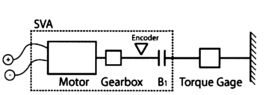
SVA

Encoder +

Motor Gearbox

Bi Torque Gage

Figure 4: System model for measuring individual damper characteristics To control for variability in the manufacturing process, the same dampers were

used in each experiment. To accurately characterize the relationship between the torque and speed across these specific dampers, a Futek TFF325 torque gage was attached between the SVA output and a rigid surface. A computer controller sent a stair voltage waveform of 0, 4, 7, and 10 volts through an Apex PA16A power amplifier circuit to drive the motor, producing a sequence of steady-state angular velocities across the damper currently mounted on the adapter plate. The turn angles measured by the encoder and the voltage produced by the torque gage were logged to a computer with a 2 kHz sampling rate.

The numerical derivative of the shaft angle as a function of time was computed from the recorded data to find the angular velocity of the damper. The torque voltage signal was initially very noisy, and was cleaned using a median filter with a window of 20 following samples. The voltage change induced by each successive applied speed was then converted to a torque value using a table of calibration values provided by the manufacturer.

A least-squares linear fit was performed on the collected values to obtain a single

characteristic ratio between torque and angular velocity for each damper.

3.3

System Dynamics Verification

To measure the steady state response of a loaded SVA system, a load consisting of a rigid shaft and a second damper was coupled to the output of the SVA, as shown in Figure (1). The casing of the load damper was held stationary, producing a load impedance proportional to the output shaft speed. A second rotary encoder measured the turn angle of the output shaft. A step input of 10 volts was applied to the motor for several seconds to allow any transient response to die away, leaving only the steady-state angular velocities of the gearbox and output shaft. The turn angles of the gearbox shaft and the output shaft were logged using a computer and differentiated to produce angular velocities as a function of input voltage. The ratio between these was computed and compared to the expected value derived from the measurements of the dampers and Equation (17).

3.4

SVA Impedance Measurement

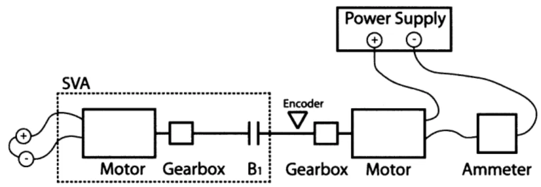
Figure 5: Setup to measure impedance of SVA.

To measure the impedance of the SVA, a second motor and gearbox set were coupled to the SVA damper as shown in Figure (5). The terminals of the

SVA

To measure the static frictional torque within the second motor, the current through the motor was decreased until the output shaft stopped turning. This thresh-old current at this operating point was recorded.

The torque applied to the SVA system was found from the recorded current as shown in Equation (1). The angular velocity of the load shaft was found from the encoder data as shown in Section (3.2). The impedance of the SVA system as a function of damper type and shaft speed was found as the ratio of the applied torque and the angular velocity, as given in Equation (20).

4

Results

4.1

SVA Design

Table 1: System constants found from component datasheets.

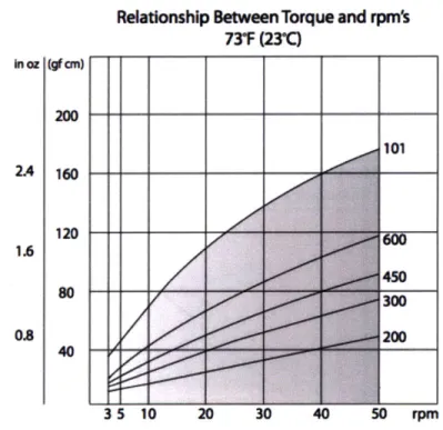
Relationship Between Torque and rpm 73'F (23'Q in m 2A 1.6 0.8 (ion) 200 160 120 so 40

Figure 6: Damper torque-speed curves as given by manufacturer. The 200, 600, and

101 grades were used in this experiment.

g 837/13

KT 0.049 N-m/A

4.2

Damper Characterization

Table 2: Damping coefficients for SVA and load dampers as a function of applied voltage (mN.m.s/rad).

Rotor angular velocity (RPM)

Figure 7: Torque-speed curve for B1H damper with least-square fit. 4V 7V 10V B1H 7.90 5.38 4.45 BiM 4.67 3.51 2.94 B1L 1.54 1.17 1.05 B2H 7.60 6.22 5.00 B2M 4.22 3.56 2.90 B2L 0.95 1.32 0.89

Table 3: Least-squares fit damping coefficients from Table (2) (mN-m-s/rad). B1H 4.73 B1M 3.14 B1L B2H B2M B2L 1.10 5.40 3.11 1.01

4.3

System Verification

Table 4: Measured w2/wi for SVA damper B1 and load damper B2.

Table 5: Expected W2/wi derived from Table (3) and Equation (17).

B2H B2M B2L B1H 0.462 0.619 0.817 B1M 0.271 0.553 0.744 B1L 0.037 0.021 0.209 B2H B2M B2L B1H 0.467 0.603 0.824 B1M 0.368 0.502 0.757 B1L 0.169 0.261 0.521

Table 6: Ratio of measured u2 and expected W2.

4.4 SVA Impedance Measurement

20 |-15 1 10 . -D---01 1 2 3 4 5 6 7 8 9

Shalt Speed (radis)

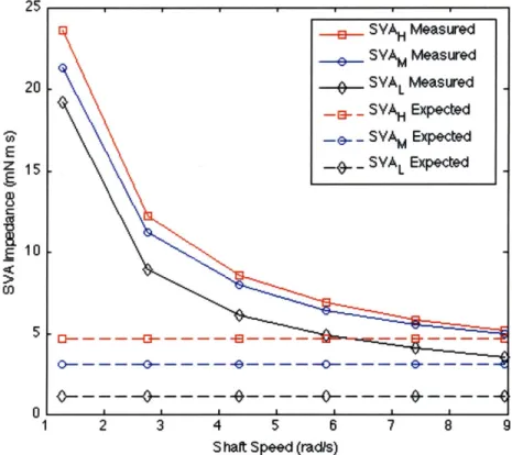
Figure 8: SVA impedance as a function of speed and damper type. B2H B2M B2L B1H 0.989 1.027 0.992 BlM 0.736 1.102 0.983 B1L 0.219 0.080 0.056 _ SVAH Meastred * SVAM Measured SAL Measured _B... SVAH Expected - SVAM Expected - SVAL Expected

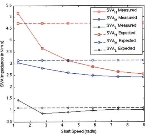
5 - 0 SYAM Measured 4.-- - -- - - 0- SYA Measured 4.5 .- L -- - SVAH Expected 4- SYAM Expected E -5-- SVAL Expected a) _{8 - - - --- - - - - - - - - -o0- - - - - e--} ---C 3 -2.5 -C 2 0.5 1 2 3 4 5 6 7 8

Shaft Speed (radis)

Figure 9: SVA impedance as a function of speed and damper type corrected for static friction torque.

5

Discussion

The damper characterization measurement produced results within a few percent of the manufacturer's data sheet. It is important to note that the expected range of operation should be considered when linearizing the damper, as the decreasing slope of the damper's measured torque-speed curve shown in Figure (7) cannot be perfectly modeled by a straight line.

The entries in the upper right of Table (6) reveal the that a medium or heavy

SVA damper driving a load of equal or lesser damping closely matches the expected

response from the model. A medium SVA damper driving a heavy load is poorly approximated by the model, and a light SVA damper behaves completely differently than expected. This is likely due to the non-modeling of dry or Coulomb friction within the system; friction has a significantly greater effect in low-torque, low-speed configurations as it is a larger percentage of the overall torque.

It was observed during the SVA impedance measurements that the gearbox output shaft did not rotate for anything except a 30 volt excitation and the heaviest SVA damper. From the point of view of the SVA damper, it acted as a fixed shaft, simplifying the system impedance to simply that of the damper itself. This result clearly follows from Equation (21) -the motor was shorted, reducing R to the internal winding resistance of the motor. Inserting the system values from Table (1) into this equation reveals an expected steady-state SVA impedance of the SVA within 1% of that of the damper itself.

As a check whether this high motor impedance was caused by a high electro-mechanical impedance or merely static friction within the SVA, the experiment was repeated with the short between the SVA motor terminals removed. It was observed that the gearbox shaft began to spin under lighter loads, indicating that a significant reduction of the SVA impedance. The derivation of Equation (21) neglected any loss mechanisms other than the motor resistance, so it predicts that the effective steady-state impedance will drop to zero as R goes to infinity. While this is clearly a deficiency of the model, the trend of reduced impedance is correctly predicted.

The primary unmodeled loss mechanism is is static friction within the SVA, most likely within the motor gearbox. The gearbox used in these experiments made use of spur gears, which are traditionally less efficient than other gearbox configurations. The effect of static friction can clearly be seen in the SVA impedance measurements displayed in Figure (8). The expected steady-state impedance is independent of the output shaft speed, but the measured impedances of three SVA configurations at low speeds range from 5 to 20 times too large. The measured impedances asymptotically approach the expected values, dropping off like the inverse of the shaft speed. This behavior can be explained by a constant frictional torque resisting the shaft motion. Figure (9) shows the same data with the measured static torque of the gearbox subtracted, and shows the greatly decreased dependence of impedance upon angular velocity.

Taking all of this into consideration, the general design procedure for an SVA should begin with an appropriate model of the system to be driven, including the load damping, the desired torques and operating speeds, and the desired SVA output impedance. Equation (21) and Figure (9) indicate that the overall system impedance is effectively the impedance of the SVA damper, so the damper should be chosen to match this desired output impedance. Once this value is determined, the necessary motor power can be chosen by back-calculation from the efficiency of the SVA given in Equation (17). The appropriate gear ratio and motor constant KT can then be chosen from the desired steady-state torque or angular velocity values given in Equations (15) and (16).

The deviations from the expected behavior resulting from very low choices of SVA dampers shown in Table (6) result from mis-modeling of the useful torque within the system. This problem may be addressed by either improving the quality of the gearbox or carefully modeling the damper and using encoders to measure wi and

W2. By increasing the gearbox quality, the losses to static friction can be largely

reduced. This will result in a transition similar to that from Figure (8) to Figure (9) and bring the low-speed impedance SVA impedance closer to the expected value. Harmonic drives are one such way to reduce the gearbox friction. Alternatively, by

characterizing the damper well and measuring the speed on either side, the torque delivered to the load can be calculated and controlled using a feedback loop. Allowing such low output impedances will allow lighter, smaller, and cheaper motors augmented with high-ratio gearboxes to meet the desired specifications.

6

Conclusion

The series viscous actuator configuration was found to be an acceptable means of reducing the effective impedance of a high-impedance actuator. The dynamic model derived for this research accurately predicted the physical response and of the system in configurations where the SVA damping matched or exceeding the damping of the driven load. The largest discrepancies between the model and the physical system concerned static and dynamic friction, which were particularly prevalent in low-speed and low-torque configurations.

Future work should focus on adapting the the adaptation of this system for use in rehabilitative robotics. As the conditions that produce significant deviations from the model coincide with the optimal conditions for use of an SVA - low speed and low output impedance - methods to reduce the losses to static friction should be investigated. Completely novel solutions may produce the best result - for example, the motor itself might be used as the vane of the damper in order to minimize the space usage of the SVA.