CCD photometric precision for the Transiting Exoplanet Survey Satellite (TESS)

CCD Photometric Precision for the Transiting Exoplanet

Survey Satellite (TESS)

by

Lulu Liu

SUBMITTED TO THE DEPARTMENT OF PHYSICS IN PARTIAL

FULFILLMENT OF THE REQUIREMENTS FOR THE DEGREE OF

BACHELOR OF SCIENCE IN PHYSICS

AT THE

MASSACHUSETTS INSTITUTE OF TECHNOLOGY

MAY 2009

ARCHIVES

@ 2009 Lulu Liu. All rights reserved.

The author hereby grants to MIT permission to reproduce

and to distribute publicly paper and electronic

copies of this thesis document in whole or in part

in any medium now known or hereafter created.

Signature of Author:

Department of Physics

A

_{. May 21, 2009}

George R. Ricker

Senior Research Scientist

-

P.I. of TESS Mission

Thesis Supervisor

David E. Pritchard

JUL

0 7 2009

LIBRARIES

CCD Photometric Precision for the Transiting

Exoplanet Survey Satellite (TESS)

Lulu Liu

Submitted to the Department of Physics on May 22, 2009 in Partial

Fulfillment of the Requirements for the degree of Bachelor of Science

in Physics

Abstract

We seek to fully characterize all noise contributions along the CCD and electronics signal path specific to the equipment to be used on board the TESS all-sky space observatory. We adjust physical variables in such a way as to minimize this noise and achieve a photometric precision limited in large part by shot noise. Ultimately, the goal is to demonstrate in the lab, by analyzing photon data generated by LED simulated stars and using relative photometric techniques, that TESS CCDs and electronics are capable of performing pho-tometry at the 100ppm (parts per million) level as required by the goals of the space mission. In our investigation, we are limited by unusually high readout noise in the CCD electronics but still able to achieve reliable sub-200ppm level photometry in the lab.

Contents

1 Background in Transiting Exoplanet Science 3

2 Introduction 4

3 Breakdown of Major Noise Sources

Limiting Photometry 5

3.1 Shot Noise ... ... 5

3.2 Dark Current ... 5

3.3 Variations in Quantum Efficiency ... . . ... 6

3.4 Saturation and Pixel Overflow ... ... 7

3.5 Readout Noise ... ... 7

3.6 Gain and A/D Converter Nonlinearlity . ... ... . 8

3.7 Error Propagation Formula. ... .... 9

4 Means and Methods 9 4.1 Data-Taking Strategy ... ... . 9

4.1.1 Equipment and Set-up ... ... 9

4.1.2 Temperature Control ... .... 11

4.1.3 Dark Current Elimination ... . 13

4.1.4 Strategy for Dealing with Pixel-to-Pixel Variation ... . 14

4.1.5 Humidity's Effect on Photometry . ... 14

4.1.6 Stability of LED Light Source . ... 15

4.1.7 Undersaturating Pixels and A/D Bits . ... 17

4.2 Analysis Strategy ... ... . 17

4.2.1 Image Stacking and Stamp-Size Subarrays . ... 17

4.2.2 Background/Bias Subtraction . ... 18

4.2.3 Star Field Intensity Profile and Relative Photometry ... . . 20

4.3 Summary ... ... .. 22

5 Calibration - CCD Gain 23 5.1 Relation to Shot Noise of a Bright Source ... 23

5.2 Calibrating to X-Ray Photons of Known Energy . ... 24

6 Photometry 28 6.1 Star Plate Layout and Star Reference Numbers . ... 28

6.2 Signal to Noise as a Function of Bounding Radius . ...

29

6.3 Intensity Correlations with Temperature and Position . ...

30

6.4 Light Curves

...

...

33

6.4.1

Shot Noise Limit? ...

...

33

6.4.2

Exclusions ...

...

.

33

6.4.3

Photometry Results ...

...

...

35

6.4.4

Analysis . . .

... ...

...

36

7 Conclusions and the Future

39

1

Background in Transiting Exoplanet Science

The first confirmed discovery of an extrasolar planet (or exoplanet) around a Sun-like star occurred in 1995 to the fascination of scientists and non-scientists aSun-like , [9] (Mayor & Queloz, 1995). Not only did the announcement touch off a new era in the human ongoing search for company in the universe, it also launched a now very exciting subfield of astronomy and astrophysics devoted to the discovery and study of these bodies. Since 1995, hundreds of exoplanets have been discovered orbiting main-sequence stars, with the rate of discovery increasing each year. The vast majority of these planets were detected through radial velocity measurements of its host star. Now, improved instrumentation has given us more powerful observational techniques. One recently expanded technique takes advantage of a somewhat rare occurrence: transits.

A transiting extrasolar planet is distinguished by the orientation of its orbit which causes it to periodically "transit" or pass through our line of sight to its host star, blocking some otherwise incident light and reducing the measured brightness of the star. Close to the star, about 10% of planets exhibit transits, but this probability decreases with both increasing radius of orbit and decreasing star size [13] (Ricker, et

al). The physics of transiting exoplanet discovery then centers around detecting these

very small, periodic changes in the intensity of radiation from a star as to indirectly determine the presence of'an orbiting body. Such a search generally monitors many stars all at once.

Ground-based surveys have contributed to the discovery of about 20 exoplanets using this technique, but are limited in sensitivity by "red noise", or noise associated with the deflection and absorption of star light by the atmosphere, to about 1%, or 10,000 ppm (parts per million) [12] (Pont, et al, 2007). Transits associated with smaller planets, with depths of less than 10,000 ppm, are lost in this noise floor, so ground-based searches strongly favor "hot Jupiters", or large planets orbiting very close to its bright, parent star. A whole new level of photometry can be achieved in space. A survey conducted in low-Earth orbit can neglect to great approximation any atmospheric effects and conduct photometry at the level limited only by shot noise from the source and CCD and electronics noise from the instrument itself. The improved sensitivity allows us to dip into the regime of earth-like planets: planets with radii several times the radius of Earth orbiting in more habitable regions. The Transiting Exoplanet Survey Satellite (TESS), set for launch in 2012, hopes to avail

itself of its location in space to directly observe the transits of approximately 1000 so far undiscovered exoplanets, greatly expanding the current database. Particularly significant is its target of nearby, bright stars for candidate exoplanets, which bodes well for subsequent ground-based followup verification and determination of other important properties such as mass, composition, existence of an atmosphere, presence of water, and so on.

2

Introduction

TESS is poised at this moment to make promising contributions to the field of ex-oplanet science. However, its ultimate success in yielding the desired number and range of extrasolar planets rests in the photometric precision of its onboard equip-ment. From the initial release of a photon by the parent star to the final electrical signal output that constitutes a measurement of this photon, the signal path, even assuming vaccuum space, is fraught with noise. The inescapable photon shot noise aside, the bulk of the noise resides in the CCD itself, as charge generated by incident radiation is stored in the potential well of each pixel and transferred row by row from the array during read out. The effects of pixel-to-pixel variation, charge transfer errors, dark current, saturation and pixel overflow, charge diffusion, and so on, all serve to obscure the true signal associated with meaningful measurement. The rest of the noise is added by the electronics during the conversion from electron signal to digital "counts", also known as ADUs, or analog-to-digital units. Two effects are most notable during this signal transfer: the addition on a per pixel basis of a ran-dom readout noise, and a systematic effect called integral nonlinearity, which is most significantly observed for CCD pixels near saturation. Each additional noise param-eter accordingly decreases the photometric precision of the observing instrument as a whole and contributes to its departure from shot-noise limited photometry.

The subsequent investigation detailed in this paper is, at its core, a full-scale characterization and quantification of all significant contributions of noise along the signal path. As a secondary objective, we will demonstrate, in the lab, using simulated stars and flight-ready CCDs and electronics, 100 ppm photometry, as required by the current mission model for the Transiting Exoplanet Survey Satellite.

3

Breakdown of Major Noise Sources

Limiting Photometry

3.1

Shot Noise

Any Poisson process, or stochastic process characterized by continuous and indepen-dent events occurring at a constant average rate, obeys Poisson statistics which states that the measured rate of occurrence of these events for any given interval of time, k, can be described by the probability mass function, which also depends on the average rate, N,

Nke-N

p(k, N)

=

(1)

Here, N is both the mean and variance of the distribution in units of counts per time. The generation of photons by stellar and electrical processes obeys Poisson statistics and therefore so does the rate of arrival of these photons at each individual CCD pixel. In the limit of large N, the Poisson distribution approaches a normal (Gaussian) distribution with a standard deviation of V. This inherent noise which accompanies any signal generated by a Poisson process is termed "shot noise". The signal-to-noise ratio (SNR) due to shot noise alone is given by,

SNR = S/N = N/vN = V

(2)

which goes up as the signal increases in power.

3.2

Dark Current

For a system in thermal equilibrium at temperature T, the probability that any particle in this system is in a state with energy E is proportional to the Boltzmann

E

factor, ekT, with k representing the Boltzmann constant. From this relationship, we can see that any system at a temperature greater than absolute zero will necessarily encounter thermal excitation and associated thermal noise. This is true of CCDs as well. CCD signals are generated by the excitation of electrons from the valence band of the semiconductor detector material into the conduction band. These electrons are collected in potential wells (pixels) and then transferred out of the active region of the CCD to be read out as current. Thermal excitation can result in positive signals which are indistinguishable from that produced by actual photons. This false signal is what is referred to as "dark current".

The amount of dark current in a CCD device is a strong function of its tempera-ture. As temperature increases, available energy increases, and dark current goes up. The band gap of the absorbing material also plays a role. The band gap energy, Eg, is the minimum energy needed to promote a valence band electron into the conduction band. The greater the band gap, the lower the resolution per pixel, the less dark current at a given temperature. Equation 3 gives the general empirical expression for average dark current, in units of electrons per pixel per second, as a function of temperature and band gap energy [1](Bely, 2003).

Nd oc Te( ) (3)

Because dark current generation is also a Poisson process, on a per pixel basis, devi-ations from average follow shot noise statistics. That is,

dc = Nd (4)

Dark current can also contribute non-uniformly from pixel to pixel, resulting in CCD structure, or systematic noise.

3.3

Variations in Quantum Efficiency

No device is 100% efficient. For a certain number of photons incident upon a detector, some of them will be absorbed, a number will be reflected, and the rest will pass right through the device. The quantum efficiency of a device is simply the ratio between the number of photons absorbed (and accounted for) and the number of incident photons, usually given on a percent basis. It is sensitive to changes in the thickness of the absorbing semiconductor material, various coatings applied to the surface of the CCD, temperature, wavelength of light, and so on.

Modern CCDs often boast quantum efficiencies peaking over 90%. By compari-son, the quantum efficiency of the human eye peaks at approximately 1%, and the photomultiplier tube at approximately 10% [4] (Howell, 2000). Although for a given device, the quantum efficiency is assumed to be uniform across all CCD pixels, this is, of course, not realistically the case. Variations in quantum efficiency from pixel to pixel are about 1% RMS, and it is this systematic variation, along with discrepancies in pixel size that contribute to the pixel response non-uniformity (PRNU) scientists aim to correct for using flatfield images.

3.4

Saturation and Pixel Overflow

Once charge has been generated within a pixel, either by thermal excitation or by interaction with incoming photons, it is held in place for the duration of the integra-tion period by an applied potential. These potential wells have a set, finite depth, and the amount of charge that can be stored in each pixel during routine operation is termed the "full-well depth". If more electrons are generated than can be contained within a pixel, the pixel will saturate at the full-well depth and some left over charge carriers will be lost while others will overflow into neighboring pixels. The result is a widening or distortion of the point spread function, which will negatively impact photometry of this object. The point spread function, or PSF, is the intensity vs. position distribution profile of photons across the pixels of a CCD due to a distant point source (in this case, a star).

Charge-carriers can be lost from unsaturated pixels as well due to charge diffusion and charge transfer inefficiencies. Charge diffusion is the migration of electrons during integration into neighboring pixels by means of tunneling or finding defects in the silicon material. The probability of charge diffusion can be decreased by increasing the height of the potential well holding the charges in place. Shifting between clock voltages in a systematic way allows a CCD to be read out along a row or column. For each pixel, the transfer process is similar to picking up a bucket of water and dumping it into another and has similar drawbacks. Largely, each time the process is repeated, there exists a finite probability of charges being lost or left behind. A CCD with a poor charge transfer efficiency (CTE) will exhibit a streak, or tail, trailing from bright objects opposite the direction of readout. Luckily, modern CCDs generally have CTEs greater than or equal to 99.9995%, and this effect can, for the most part, be ignored.

3.5

Readout Noise

During readout, the accumulated charge within a pixel is first transferred to the serial register, a row of inactive pixels whose sole function is to assist in the readout process, and then the signal is sent to be amplified and converted into a digital number. The amplification is facilitated by an on-chip amplifier and the conversion by a device termed the analog-to-digital converter. The noise acquired by the signal as it makes its way through the processing electronics is random on a per pixel basis and establishes the noise floor for a CCD device. Readout noise is the term given to

the total error introduced by this whole family of contributors. One of its components is Johnson Noise, or thermal noise generated by the amplifier and other electronics, which obeys the relation [11] (Nyquist, 1928),

2 = 4kBTBRout (5)

Here, ae- is noise in electrons, kB is the Boltzmann constant, T is the temperature,

B is bandwidth in Hz, and Rout is the effective resistance of the device. The only

other noise I will mention here is "flicker noise", also known as "l/f" noise for its inverse power-law dependence on frequency. It is present in almost all electronic systems and has been documented even in biological and geological phenomena. "1/f" noise dominates readout noise in devices with slow read rates (fread < 1 MHz). Its

origins are as of yet unconfirmed, although various hypotheses have been put forth [8] (Lundberg, 2002).

For our purposes, we will treat read noise wholistically and as a constant, random, source of error in our analysis. Like all other errors along the signal path, we will look to characterize it experimentally, and minimize its effect on photometry.

3.6

Gain and A/D Converter Nonlinearlity

Our final note on error contributions belongs to systematic nonlinearity in the A/D converter. Integral nonlinearity specifically is of interest to our project. To under-stand why it is so insidious, it is necessary first to introduce the concept of gain. The gain of an A/D converter is the conversion ratio between the signal in electrons and the output in ADU's or Analog-to-Digital Units, and is set by output electronics starting with the on-chip amplifier.

Gain = (6)

ADU

The gain of most CCD electronics is between 1 and 20 electrons per ADU. The relationship is linear, i.e. the gain is constant, over nearly the full output range of the A/D converter, but has a slight dependence on temperature. The linear region is the useable dynamic range, where a value in ADU can be easily associated with the number of charge carriers generated within a pixel. For pixels near but below saturation, however, the behavior is harder to predict, we've entered the region of nonlinearity. While there are clear signs which alert us to the likelihood of saturation in the A/D converter and pixel full well, nonlinear pixels raise no red flags. An

experimenter who converts the value in ADUs of these nonlinear pixels into electrons

using the gain as the conversion factor would get systematically erroneous results.

It is often best to avoid working in this region altogether. For example, in a 15-bit

A/D converter, the largest usable output is usually taken to be around 25,000 ADU

[4] (Howell, 2000).

3.7

Error Propagation Formula

Propagation of random errors on statistically independent quantities is governed by the very important error propagation formula. I will repost it here because of its

centrality to much of our analysis. Given a function f(x, x2,...) of independent variables x1, 2, ... with associated uncertainties x,X ₂, ..., the uncertainty on f,

represented by af obeys [2]

2 =

=f

(Of

_a

+

(7)

All the errors given above can be thought of as associated with independent

vari-ables.

4

Means and Methods

4.1

Data-Taking Strategy

4.1.1

Equipment and Set-up

The investigation is conducted using equipment and facilities belonging to the MIT

CCD Laboratory located on the fifth floor of the Kavli Center for Astrophysics

Re-search (Building 37) at MIT. We gather data using a 2000 x 4000 pixel back-side

illuminated frame transfer CCD manufactured by Lincoln Laboratory. Pixels are 15

microns on a side. Electronics are designed by the MIT CCD Laboratory for use with

an 18-bit A/D converter (a switch from the 12-bit to the 18-bit converter occurred

about halfway through this investigation, all essential measurements were repeated

using the new system). We use the lower 16 bits of the A/D converter. Integration

time is about 1 second per exposure. The chamber housing the CCD is kept near

vacuum at - 10-6 atmospheres; we tune its temperature by careful adjustment of

the flow of liquid nitrogen into the chamber. The CCD is fitted with an 85 mm, f/1.2

camera lens with an adjustable focus. One meter away, a power LED serves as our

Turbo Pump Front Plate Star Plate

/

\4

-Im

Figure

Figure

light source. It is placed behind a "star plate", that is, a thin metal sheet dotted with

precision-drilled micrometer-width holes, and together they are mounted on a 3-axis

programmable motor drive capable of simulating spacecraft jitter.

The path from the star plate to the lens is shielded, to the best of our abilities,

from infrared and visible light. Output from the CCD is read by a Linux machine and

compiled into FITS (Flexible Image Transport System) files for subsequent analysis.

Diffuser

LED

4.1.2 Temperature Control

The various dependencies of essential system parameters (such as gain and dark current values) motivate our desire to have precise knowledge and management of the temperature of the CCD system.

A Platinum Resistance Thermometer (PRT) placed inside the chamber near the CCD plate monitors, to good approximation given equilibrium conditions, the tem-perature of the plate itself. The conversion from resistance to temtem-perature in Kelvin occurs internal to the Lakeshore temperature control device itself, while an IDL script compiles the output, recording temperature as a function of time.

Two methods for exacting control over the temperature of the CCD are used. Method one involves a heating function built into the Lakeshore device, and an inter-nal feedback loop to activate and deactivate the heater based on the comparison of the temperature readout to a set point temperature, or "goal" temperature. Liquid nitrogen flow is steady, governed by a programmable timer which opens and closes the solenoid valve along the liquid nitrogen pipeline. The heater-timer method has the advantage of shorter period and lower amplitude temperature fluctuations in its equilibrium state (as short as a few seconds depending on the setting on the timer, and as low as 0.2K), but has the disadvantage of direct heating of the CCD, which, depending on the location of the temperature probe relative to the active heating mechanism, may yield unpredictable results due to uneven or local heating, such as a temperature gradient in the CCD or an inaccurate temperature reading. This method runs through nitrogen at a quicker pace, which limits the total number of data points with which we can construct a stable light curve.

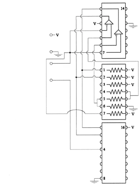
A second method takes input from the PRT, passes it through a simple logic circuit (Figure 3), and outputs instructions to the solenoid valve which controls nitrogen flow. It uses no heating mechanism aside from thermal contact with room temperature environment, and the set point is a range as opposed to a single value. The chamber temperature readout is compared with two bounding temperature values by way of a comparator, and the device will act to keep the temperature within this range. The range itself is set by a network of resistors and one adjustable potentiometer. This method has as its advantage even warming/cooling of the CCD and a more reliable temperature reading due to affecting the large-scale temperature control mechanism rather than combating its effects on a local scale (treating the cause, rather than the symptoms, so to speak). However, it is not without its drawbacks as the nitrogen must flow through the piping in order to begin cooling the CCD, the thermal inertia

of this system is rather large and we are looking therefore at a slower response rate.

Using a range of temperatures as a set point rather than a single value, although

essential for the correct operation of the circuit created especially for this purpose,

also acts to increase both the amplitude and the period of the temperature oscillations

to approximately 1K and 3-4 minutes, respectively.

Figure

3:

4.1.3

Dark Current Elimination

The strong dependence of dark current on temperature is good encouragement to

work in a very low temperature regime. Of course, since dark current is zero only

at absolute zero, we are not looking to eliminate it completely. Instead, we look to

establish a level for the dark current such that the shot noise resulting from the dark

current is insignificant compared to the readout noise and other baseline,

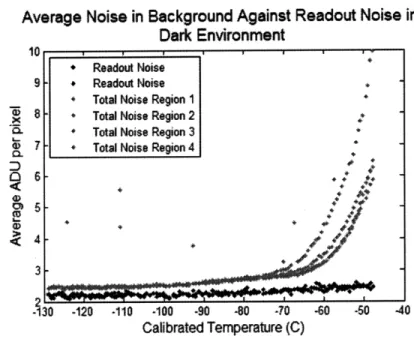
temperature-independent sources of noise. Figure 4 plots the total noise in an unlit region of the

Average Noise in

Background

Against Readout Noise in

Dark Environment

10 1 f I I I I

* Readout Noise 9 * Readout Noise

* Total Noise Region I

' 8- * Total Noise Region 2 .

* Total Noise Region 3 * e 7 * Total Noise Region 4

3--130 -120 -110 -100 -90 -80 -70 -60 .50 40

Cafibrated Temperature (C)

Figure 4: Comparison of total pixel-to-pixel variation of several regions in a dark frame of the CCD to the variation in the overclock region (readout noise only), as a function of approximate temperature.

CCD against the temperature of the device.

It becomes immediately evident that below -110K, dark current noise disappears

behind a dominant, temperature-independent noise term which is slightly larger than

the readout noise of the electronics as measured in the overclock region of the CCD

by a fraction of an ADU. The divergence of the noise in different regions in the high

temperature zone indicates structure in the CCD pixels, and the asymptotic difference

between readout noise in the active region of the CCD and in the overclock region is

closely related to a bias offset which for this CCD, could not be reduced any further.

It is important to mention that this data is collected on a 12-bit converter and a test

CCD for the purposes of developing experimental strategy early on, and the later

photometric data is actually taken with a similar but more advanced CCD and set of electronics.

4.1.4 Strategy for Dealing with Pixel-to-Pixel Variation

The measured pixel-to-pixel RMS deviation in quantum efficiency is 0.8% for the actual CCD used in the following experiment [16]. In addition there is often minor structure in the noise or the dark current generated on a per pixel basis due to

variations in pixel size or in the material itself. Although seemingly insignificant, these pixel-to-pixel variations are what mandates the practice of "flat-fielding". Flat-field images, usually taken of a uniformly illuminated surface such as a white wall, give us all the necessary information to normalize out all noise contributions of this nature from our data frames.

Because of the nature of our eventual mission, we neither have the flat-fielding capabilities we have on the ground (no moving parts on spacecraft bus, no large, uniformly lit regions in the sky) nor do we need them. We are merely looking for changes in a star's total incident intensity. Therefore, if we can keep the spacecraft attitude fixed to within a couple of arcseconds, we can keep the major portion of each star's point spread function (PSF) over the same few pixels, and will not need to attempt to flat-field in space. Strangely enough, we will find that our pointing accuracy and the steadiness of the attitude of the camera and CCD is probably better in space than in the lab. Nevertheless, we adopt the technique of fixing the array of stars to the same position on the grid of CCD pixels for each image as a way of eliminating pixel-to-pixel variation.

4.1.5 Humidity's Effect on Photometry

During the summer months, especially, humidity is an issue in the Boston area. When untreated, condensation begins collecting on the window of the liquid-nitrogen-cooled chamber behind which is situated the CCD. Of course, water droplets deflect

and reflect incident light, and the presence of this condensation can severely impact photometry. Our remedy is dry nitrogen. A steady flow of dry nitrogen over the chamber window, initiated before the liquid nitrogen, is sufficient to remove this worry from our minds.

4.1.6 Stability of LED Light Source

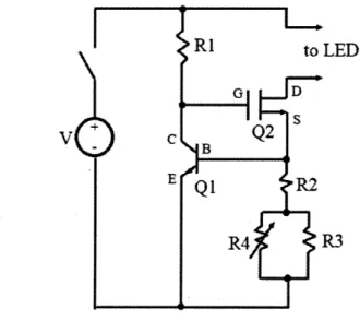
Since every variable is a potential source of noise or error in our investigation, it is also important to be able to fully control the brightness of the power LED light source. Originally, a voltage-source circuit supplied the power to the LED and the LED was operated at the very lowest end of its capabilities due to limited full-well capacity in the test CCD and a 12-bit A/D converter. Early data showed disturbing, high amplitude, apparently random fluctuations in the brightness of stars in the star plate on the timescale of hours (see Figure 6).

R1 to LED

V

C

Q2

B

E

Q1

tR2

R4 R3

Figure 5: Constant current source circuit diagram. R1 is a 100 kQ resistor, R2 a 120 Q resistor, R3

a 1 kQ resistor, R4 a 5 kQ potentiometer. Q1 is an NPN transistor, Q2 is an N-channel MOSFET.

After ruling out possible causes including humidity (as discussed in section 4.1.5 above) and correlations with CCD temperature, we realize the culprit is likely the light source itself and make two crucial corrections. First is the design of a very basic, constant (but tunable) current source (see Figure 5). Then, the brightness of the LED is cranked up to normal operating levels while its signal is accordingly dimmed by two constant-density filters. This allows us to continue to operate in the undersaturated regime of our instruments and stable range of our LED at the same time. Stability was much improved after these changes were implemented (see Figure 7).

x 10< 35-f 3 C_t S2.5 2 () gs C 0₃ 00 05

Light

Curves for 15 Stars

5 10 15 20 25 30 35

Successive Sums of 100 Exposures

Figure 6: Early light curves for 15 stars using 12-bit electronics. Evidence of an unstable LED

source.

x

Raw

Light

Curves for 13 Stars

1

0 2 4 6 8 10 12 14 16 18 20 Successive Captures (500 Exp Sum)

Figure 7: Light curves obtained after changes were made to the LED power source and operational parameters. No normalization has taken place.

4.1.7

Undersaturating Pixels and A/D Bits

We take pains to avoid saturating the full-well of a pixel or the A/D converter in order

to avoid many of the problems introduced in Section 3 which become manifest in this

region. Our strategy in general will be short exposures and low-intensity signals, and

relying on stacks of individual image frames to produce the statistics necessary to

reach our photometry goals.

4.2

Analysis Strategy

4.2.1

Image Stacking and Stamp-Size Subarrays

FITS format output produced in the readout process is an array of signal values in

ADUs which preserves the location of the pixel on the CCD that had collected it.

This makes image stacking a simple task, as the value of a particular pixel in any

exposure can be found each time at a fixed location in the array. Analysis scripts

are equipped with the ability to take simple sums over many FITS arrays along each

element in the array in order to produce stacked images which hopefully reproduce

the photometry of much brighter objects.

An onboard data reduction technique planned for TESS, which would reduce

dramatically the data downlink load, is the use of image subarrays. Eventually, a

4W0 4610 4620 4630 4640 4650

Figure 8: 40x40 pixel subarrays generated from full CCD frame. 4660 4670

program will locate the centers of stars suitable for photometry, draw a certain sized

box around it, and save only these stamp-size arrays for analysis. For now, we choose the star centers by hand, since this only needs to be done each time the star plate is shifted, and leave the rest to a computer script.

The script reads in the list of star centers, takes 20 pixel-steps in each direction from these locations, and throws down a 40 x 40 pixel frame around each star of

interest. These subarrays are saved in a separate file for subsequent analysis. An

example of nine stamp-size subarrays is shown in Figure 8.

4.2.2

Background/Bias Subtraction

There are many ways of finding the background-subtracted intensity of a star in a

subarray. For very precise measurements, one may desire to fit the point spread

function of the signal on the CCD to a gaussian, or even better, an Airy disc for

diffraction through a circular aperture, defined by

I(r) = Io 2J(r)

(8)

where J

is the first order Bessel Function, and Io and a are fit parameters. There

is much complexity to PSF fitting and it is even more complicated by the distortion

of the PSF due to non-central location in the field of view, an example of which is

given below in Figure 9, data from Howell, 1996 [4]. For our current purposes, the

marginal improvement in photometry is not worth the added processing time and

complication; instead, we go with a simple sum. The program finds the peak pixel in

each subarray and draws another bounding box of specified radius b. It then sums the

values of all the pixels contained within this smaller photometry box. To determine

background, it does a 300 pixel sample of the perimeter of the subarray and calculates

the average value of these pixels "far away from the star". This same value is then

subtracted on a per-pixel basis from the signal pixels within the central photometry

box. The operation is summarized below, where Ibs is the resulting

background-subtracted intensity of the star.

4b2

Zbs =

S

i=0

Here,

is the signal (in ADU) collected from the ith pixel within the photometry

box of radius b, and Sbg is the average background level set by a sample of 300 pixels

PSF va to arors Ie Field of View

0

0 1 2 n12-1 n12 n21 n-2 n-I n

Figure

along the perimeter of the full 40 x 40 subarray. 4b

_{is just the total number of}

pixels. This method eliminates the need to take bias or dark frames, and allows us

to observe parts of the sky with very different temperatures and background photon

levels at the same time. With a consistent method of simultaneous local background

and bias correction, the mission is afforded a greater observing flexibility and freedom.

Sph,i has two main contributions that we need to be concerned with, incident photons

and bias. The uncertainty on Ibs can then be found by using the error propagation

formula, Equation 7, assuming shot noise error on the actual bias-subtracted signal

and approximately uniform illumination of each background pixel.

b = Ibs

+

+ 16b

_a-

Ibbs b 4bb (10)

The error on the mean background depends on the readout noise

and the

number of pixels used in the calculation, N.

Sbg (11)

Equation 10 becomes:

9ibs = s, + 4b2a + 4( (12)

Later, b will be optimized for signal-to-noise ratio, or Ibs/-lbs.

4.2.3

Star Field Intensity Profile and Relative Photometry

Relative photometry is a useful technique for eliminating wide-field fluctuations in signal intensity. Though it is more crucial in ground-based exoplanet surveys than in space, it is useful in all contexts involving CCD electronics as it removes the effects of common-mode rejection in amplifiers [7] as well as temperature-dependent variations in the system gain, which uniformly affects all signals. We will find that in our investigation, in particular, due to the nature of our light source, it is indispensable. We model our light source as an isotropic emitter. A diffuser is placed a distance

d ? 1.5 cm away from the source, and the star plate approximately 2 inches from the

diffuser. It is immediately obvious our star field will not be uniformly illuminated.

z

to CCD

Diffuser

LED

Light Source

Figure 10: Geometry and coordinate designations used to calculate intensity profile for stars in star plate as a function of p, distance from the z-axis.

The brightness profile of the stars on the star plate will mirror the distributed intensity of light incident on the diffuser placed behind it. Ideally, as a function of polar distance

p from the centroid of the symmetric profile (£ = (0,0,0) in our coordinates), intensity

I is described by the function

Ptotd 1

= 4r

(d

where Ptt is the total power radiated by the LED light source. A plot of a cross section of this intensity profile as a function of distance from the z-axis is shown in

Figure 11. 0.8 -0.6 -0.4 - 0.2--3 -2 -1 1 2 3

Figure 11: Projected intensity of light onto a planar diffuser from an isotropic source as a function of radial distance p. The profile is reflected across the vertical axis to emphasize circular symmetry.

This function is linear in Ptot, which tells us that a constant factor increase in the brightness of the LED results in the same constant factor increase in the brightness of every star in the star field. Fluctuations of this nature can be corrected for by relative photometry.

Relative photometry is normalized photometry. Each star's total signal in elec-trons is converted into a unitless ratio by comparing its value against some reference value. There is some freedom in the choice of this reference, and clearly some choices are better than others. For one, it should not be a constant, but vary accordingly with the stars in the field. It should be some reliable characterization of the overall photometry. For these reasons, we choose as our reference value the average intensity

of all stars of photometric interest in the frame.

Ii

Ii-

(1/M) EM1 i

Ri is the relative brightness value of star i, Ii is brightness in electrons, M is the num-ber of relevant stars in the field. The uncertainty on Ri, propagated using Equation 7, is then

2 (1)2 (15)

with I representing average intensity. Putting them together to find an expression of normalized noise introduced by this method of photometry, we find,

-R,/Ri = i () 2 (16)

ai is calculated by the photometry software alongside Ii, ay is given below.

=

S

2

(17)

j=1

These equations are central to our strategy of relative photometry. As an aside, if we assume Poisson statistics (which is very idealized, of course), the relative signal to noise ratio, aRj/Ri, reduces to

UR,/Ri =- -

)

We confirm the intuitively reasonable assumption: that the photometry is limited by the number of stars, M, involved in the mean. In order to control the error introduced by normalization, M should be as large as possible.

4.3

Summary

We have most of the tools we need to begin our study. The code required to implement the functions described above is written in a number of languages, including Matlab, IDL, C, and Shell script. It's important, however, before we begin, to review the procedure as it has been presented so far as well as introduce the desired format for our results. Light travels from the light source to the diffuser, through the holes in

the star plate, along a light-shielded path, into the lens which focuses the photons onto the pixels of a CCD in back. The CCD is held at a temperature of -120K or below and read out approximately every second. The electrons collected in each pixel are transferred and converted by an A/D converter into ADUs and stored in FITS files for analysis. Analysis begins by stacking the images in chronological order in groups of 500 or more for improved statistics. Star centers are picked out and subarrays generated for each star in each stacked frame to facilitate data transfer and storage. Each star has an absolute and relative brightness in each frame sum, which is to be compared with its own values at earlier and later times. An RMS deviation of the relative intensity is measured, and inspected for its resemblance to expected error (aRj calculated from the parameters of the experiment) and shot noise limit of each particular star. Finally, all these uncertainty values are given as fractions of the average intensity of the star, multiplied by 106 to give parts per million statistics.

5

Calibration

-

CCD Gain

As with any experiment, calibration of the equipment is essential before any interpre-tation or analysis of the data can take place. A parameter of utmost importance when working with output from CCD electronics is gain. A more detailed introduction to gain can be found in Section 3.6, but suffice to say, it is most straightforward and reliable to determine the gain of the system by measurement rather than calculation. Several established methods exist. I will describe two of the simplest and one of those in detail as it is carried out.

5.1

_{Relation to Shot Noise of a Bright Source}

The first of these methods takes advantage of shot noise statistics and the relationship between number count of incident photons and numerical output in ADU. In the visible light and infrared region of the spectrum, one photon is universally correlated with the creation of one electron-hole pair [14]. The conversion between units of ADUs and photon counts is then,

NADU = N/g + Bias + NDc/g (19)

where g is the gain of the system. Bias is in units of ADU, and dark current, NDC, in units of electrons to facilitate in calculation of Poisson noise (see Section 3.2). Since

the number of photons obeys shot noise statistics, we can calculate the noise per pixel in ADU, UADU. It is a function of photon signal, N,, readout noise in electrons, aR, and dark current in the pixel, NDC.

2ADU

+ + NDC (20)

in the region where N, >> Bias and NDC, Equation 19 reduces to

NADU N1/g (21)

and the noise becomes

1

ADU -

N

(22)

converting N, in photons into units of ADU we plug Equation 21 into Equation 22 and obtain

1 NADU (23)

0ADU - NADU

g g

which is decidedly not Poisson in nature unless g = 1.

This key relationship can be exploited to determine the gain, g, from histograms of pixel values by analyzing either one very bright, very uniformly illuminated flat field frame, obtaining UADU from the RMS variation from pixel to pixel, and NADU as the mean value of all pixels, OR taking multiple exposures of a single, steady, bright source, and extracting aADU and NADU from single pixel variation from frame to frame.

We went into a bit of detail in discussing this method because of the important relations introduced. Equation 20 in particular, is the crucial noise component of the ubiquitous "CCD Equation", in units of electrons,

S N

N

N

N

+

ND

5.2

Calibrating to X-Ray Photons of Known Energy

Scholze, et al, found in 1996 [14] that the average electron-hole pair creation energy in silicon is 3.64 eV for excitation by photons in the x-ray range. Iron-55 decays into manganese-55 by inner-shell electron capture and the resulting cascade of higher energy electrons into lower energy orbital states to fill in the ground state of the manganese atom releases a bundle of x-rays with highly specific energies. The Kc,

line emitted by the decaying Fe-55 atom corresponds to the 2p

--

s transition and has

an average energy of 5.9 keV. The K3 line corresponds to the 3p --+ ls transition and

has an average energy of 6.5 keV [10]. The corresponding number of charge carriers

created by the absorption of a single x-ray photon is 1621 and 1786 respectively. If we

then measure the ADU output by the CCD corresponding to these individual events,

we can very easily take their ratios and obtain the gain of the system.

The front plate to the vacuum chamber containing the CCD is removable and

interchangeable. For photometry purposes, the front plate is fitted with a camera

lens to focus photons from the light source onto the CCD. For gain determination,

this front plate is removed and replaced with one fitted with an Fe-55 x-ray source.

The chamber is light sealed with the exception of the x-rays. A 1 second integration

of a portion of the illuminated CCD is shown in Figure 12.

Figure

Figure

A single absorption event on the CCD shows up in the read out in several common

ways, see Figure 13. All the energy of the photon is either absorbed by one pixel

(single-pixel event), or it is spread out among several neighboring pixels

(multiple-pixel event). This means, any (multiple-pixel participating in an event can contain anywhere

from 0 to 1621 (or 1786) electrons.

Since the sum across all pixels in an event should reflect the total energy of the

photon impact, some scientists opt to create scripts which would identify single and

multiple pixel events and sum them to produce the total signal in ADU. A histogram

is then created depicting the distribution of this signal sum across all identifiable

events. Hopefully, the statistics will be normally distributed. A gaussian fit then

reveals the mean.

Unfortunately, the few times we tried, this procedure did not produce much in

terms of identifiable peaks. We reverted to a much simpler approach, which actually

turned out some clearer results.

K K Ipeaks

107

10 1

-400

of Fe-55 Source Visible in CCD Histogram of Individual

-200 0 200 400 600

Pixel Pulse Height (AD

Pixel Values

800 1000 1200 1400

Figure 14: Histogram of count against pixel value (in ADU) in x-ray calibration exposures. The Mn-55 Ka and KO peaks are clearly visible. The largest peak centered at 0 ADU is the result of bias subtraction. The readout noise is measured to be 28.4 electrons.

t 1 "J f~ lj

i f

I

t

1

Although any pixel involved in an event is more likely to contain some of the

energy rather than all, when arranged in terms of signal values and frequency of

occurrence, a pixel is more likely to report the value associated with a single-pixel

event than any other specific value. In addition, we expect a step-like behavior, such

that above certain energy thresholds, more precisely, the two main energy values

taken on by the photons, the count will drop significantly as possible contributing

photons diminish. Any signal above the energy of the Kp peak is either from even

more energetic transitions or cosmic rays.

K, K. peaks of Fe-55 Source Visible in CCD Histogram of Individual Pixel Values lot [A) Peak: 0 ± 0.0 Width: ~14. 2

16, V

15 ADUO -~ausi Fit to Peak (Al ADU - aussian Pit to Peak [B]

'" Gaussian Fit to Peak [C]

Peak: 824 ± 10 ADU

Ec±

SPeak:

I I ! I I - !

--200 0 20 400 600 800 1000 1200 1400

Pixel Pulse Height (ADU)

Figure

Peak [A] is the bias, peak [B] corresponds to the Ka line of Mn-55, and peak [C] to the Kp line.

The histogram in Figure 14 is produced from the individual pixel values obtained

in 100 exposures (not stacked), with bias determined by a gaussian fit to the

zero-signal (largest) peak and subtracted individually from each frame. Individual peaks

are fit to gaussian functions, their means extracted. The width of the bias peak at 0

ADU is a good indicator of readout noise, which in this case is 14.2 ADU. Figure 15.

1620/(824

+

+

+

We find the gain of the system to be around 2 e-/ADU. The readout noise in electrons

is then a very high 28.4.

6

Photometry

6.1

Star Plate Layout and Star Reference Numbers

For the purposes of photometry, we are most concerned with stars near the center of

the field of view. PSF abberation is lowest in this region (Figure 9), and brightness

most uniform among the stars (although as we see it is still not very uniform at

all). We window only the region of the CCD which contains our stars of interest. The

motivation is reduced requirements on processing time and disk space. The windowed

region is shown in Figure 16 with the candidate stars labeled by number.

Figure 16: Candidate stars participating in photometry are referenced by number in no particular order. Brightest stars are near the center of the distribution.

6.2

Signal to Noise as a Function of Bounding Radius

In Section 4.2.2, we discussed our strategy for extracting absolute intensities of stars

by the use of bounding boxes and background subtraction. If you recall, our scripts

locate the brightest pixel in a stamp size subarray and draws a bounding box of

radius b around it, considering as signal only the pixels contained within this box,

and subtract from it the background and bias contributions in order to determine

background-subtracted intensity.

Thus, the choice of b plays a major role in the level of photometry we can hope

to achieve. Thinking about limiting cases only, it makes intuitive sense that as b

approaches zero, our signal to noise will drop to zero. On the other hand, as b

approaches the radius of the subarray, signal will stay constant as noise increases

(Equation 12), and signal to noise will decrease. A continuous function that increases

then decreases will have a maximum somewhere in between, we can optimize statistics

while holding all other parameters constant if we operate at this bo.

to Noise Ratio Curves for 19 Stars (2000 exposure sum)

"0 5 10

Radius in Pixels of Bounding Box

Figure

The value of bo depends on the width of the point spread function. Therefore, we

seek to determine b

experimentally by comparing the value of Ibs/Crbs for increasing

values of b.

We verify the behavior we expect based on the parameters we were handed. We

find that most stars peak at a relatively large b

=

9 while the brightest stars peak at

an even larger radius. Since their photometry is not much compromised, we choose

bo = 9 for subsequent photometry operations on all stars in the frame. We can be

assured that as long as the light source, the focus, and the integration time are all

kept relatively stable, we will not need to repeat this analysis.

6.3

Intensity Correlations with Temperature and Position

In the course of our study we ran into a very strange correlation between temperature

of the CCD and the x-y location of the centroid of the star on the pixels of the CCD.

We learn from our analysis (Figure 18) that this fluctuation was on the order of a

tenth of a pixel, and the orientation of this motion was different enough from star to

star to lead us to believe that it was the result of a rotation of the CCD.

At the time we were using the external temperature control circuit and the heater

was off. The temperature oscillated periodically between the two preset turning points

with a period of approximately 3 minutes and an amplitude of one degree. We were

skeptical that a change in one degree would result in such a noticeable rotation of

the CCD in the chamber, but noticing an asymmetry in the shape in the periodic

deflection, realized it must be correlated with the on/off action of the nitrogen rather

than the temperature measured on the CCD itself.

The chamber is fed by a flexible metal hose which is affixed to the side of the

CCD. Although the period of their oscillations will be the same, the hose which is in

direct contact with the nitrogen is subject to much greater extremes of temperature

than is the near equilibrium of the chamber. Large and sudden swings in temperature

have a dramatic effect on material properties, a small tensing of the tube is enough

to generate jitter at the level we observe.

Much more troubling is the effect of this jitter on photometry, as it was much

more pronounced than would be predicted by mere pixel-to-pixel variation in quantum

efficiency. Photons from a bright star are spread out over many pixels (its photometry

is built from 81, for instance), the worse case scenario is that all these pixels are

unique from frame to frame, corresponding to a jitter of more than 18 pixels. In that

case the variation in photometry due to pixel response non-uniformity will be on the

order of 1%/ i, or 0.1% [15]. Our observed brightness fluctuations for the star

10 Total Brightness vs X- Y- Position of Star 11

1.76 c1.74 -1.72 92 94 96 9 100 102 23.2 S23.1-a 23 22.9 1-92 94 96 98 100 102 22.4 -" 22.2 22 92 94 96 96 100 102

Successive Captures (no stack)

Figure 18: Temperature-correlated periodic displacements in centroid position of a bright star on the CCD. Because the star is near saturation, we observe that its background-subtracted intensity is highly impacted by this small change in position.

X 10Total Brightness vs X- Y- Position of Star 10

6.4 6.2 -92 94 96 96 100 102 22.3 g 22 1 222 9

VYVV

Successive Captures (no stack)

Figure 19: The intensity of fainter stars appear to be uncorrelated with movements on the order of a tenth of a pixel.

whose statistics are given in Figure 18 is an order of magnitude greater, while our measured jitter is more than two orders of magnitude below that which is used in this calculation. When we look away from the bright stars, we see this effect disappear entirely behind shot noise, Figure 20, which hints that this is likely an issue associated with saturation. A more detailed look at a fainter star can be found in Figure 19.

We speculate that there is clipping of the bright pixels or other loss of charge associated with nonlinearity.

x 10 A 0 0 o C Ile M CD) 3

2

Raw

Light

Curves for

19

Stars

550 600 650 700 750

Successive Captures

800 850 900

Figure 20:

coupling.

Brighter stars are disproportionately affected by this anomalous intensity-position

As the stars move around, the point spread function remains approximately con-stant while the pixels shift underneath it. This could make the difference between distribution of peak intensity over several pixels and a situation where the peak value falls squarely on one pixel. In the latter case, clipping (or charge loss) would be more severe, and a dip would be seen in the light curve of the integral intensity of the star each time it oscillates between these two states.

1' 500 __ r _______~1 ____~1____7______ ____ ___ 1__~_____1___~_ ____. L~z~L~ r t t 1 I I I

8f

Toning down the light levels and excluding from our photometry the brightest stars that exhibit this phenomenon, we ultimately construct a seven point light curve based on stacks of 2000 images.

6.4

Light Curves

6.4.1 Shot Noise Limit?

With such a high readout noise level (e 28.4 electrons, Figure 15), we struggle to reach shot noise limited photometry. We modify Equation 12 to find uIo,,, the photometric noise when working with stacks of 77 images with constant intensity, I, in each frame. We drop the background-subtracted subscripts for clarity's sake, as it is assumed that all stellar intensities are background-subtracted. The major adjustment is the dependence on 27,

,t(71)

+

(1++)

shot noise limited photometry, where , -o\ It and Itot = l71, we would need to

collect Itot >> 1 x 109

electrons. If we attempt to accomplish this by frame stacking, doubling 77 would double the intensity, but at the same time would double the readout noise component under the radical, and their contributions to the total noise remain at the some proportion as before. This implies stacking is generally ineffective for the purposes of bringing our stellar photometry closer to the shot noise limit. However, all is not lost. Meanwhile, the ratio rtot/Itot, our fractional noise, does decrease as

1/v , so stacking has a positive effect on our photometry in the expected way.

lt,

/to

I+ 4b

_{a- 1 +}

iN)

(26) All of this is easy to see graphically. Figure 21 compares our fractional noise (Equation 26) with shot noise statistics as a function of 77, the number of frames in a stack. Approximate values were entered for all constant parameters.

6.4.2 Exclusions

Although, due to the high readout noise of the system, we cannot hope to get any nearer to the shot noise limit by summing, we still attempt to stack enough images

0.0005 0.0004 Shot Noise Limit Predicted 0.0003 - SNR curve 0.0002 -0.0001 , 0 200 400 600 800 1000

Figure 21: Although the two normalized noise ratios both decrease as 1/v-j, the two curves

asymptote to different values.

so that 100ppm _{photometry is experimentally verified. If so, we can be assured that,}

in the future, when the system is tweaked to a state with a lower noise floor, which is easily done with the attention of any CCD expert on the TESS team, photometry can only be improved (and dramatically).

We are judicious in our choice of candidate stars. Keeping in mind the effect of the image jitter described in Section 6.3 on the photometry of bright stars, we exclude from our relative photometric analysis the four brightest stars in our field of view: stars 5, 6, 10, and 11 in Figure 16. These are all nearest the light source at the center of the star plate.

In addition, Star 2, the star farthest from the line-of-sight center, is also excluded due to unreliable photometry, the cause of which may be PSF aberration or overall low intensity. The rest of the stars are required to establish a reliable mean intensity curve against which all individual light curves are normalized. Recall that M, the total number of stars used to calculate the reference mean intensity, should be made as large as possible to limit error. The best statistics, naturally, will be found among the brighter stars.