Capital expenditures in industrial properties

Capital Expenditures in Industrial Properties by

Stephen James Gallagher B.Arch., Architecture, 2008

University of Notre Dame

Submitted to the Program in Real Estate Development in Conjunction with the Center for Real Estate in Partial Fulfillment of the Requirements for the Degree of Master of Science in Real Estate Development

at the

Massachusetts Institute of Technology September, 2018

2018 Stephen James Gallagher All rights reserved

The author hereby grants to MIT permission to reproduce and to distribute publicly paper and electronic copies of this thesis document in whole or in part in an' medium now kow or hereafter created.

Signature redacted

Center for Real Estate

Q L.

Certified

by_Signature

redacted

Professor David Geltner

Professor of Real Estate Finance,

Department of Urban Studies and Planning Thesis Supervisor

Signature redacted

Certified by

A exan van de Minne Re ch Scientist, Center for Real Estate Trn\is Co-fupervisor

Signature redacted

Professo''benkir'enchman

Class of 1922 Professor of Urban Design and Planning,

Director, Center for Real Estate _{MAS$ACHUSETTS INSTITUTE} School of Architecture and Planning OF TECHNOLOGY

Capital Expenditures in Industrial Real Estate

Stephen James Gallagher

Submitted to the Program in Real Estate Development in Conjunction with the Center for Real Estate on July 27, 2018 in Partial Fulfillment of the Requirements for the Degree of

Master of Science in Real Estate Development

Abstract

Using a sample of 1458 industrial properties with 36,450 quarterly observations, we apply a pair of OLS models to predict property-level NOI and capex. We then synthesize the results by modeling capex as a fraction of NOI, which we treat as a measure of property capex performance.

We model capex and NOI with a series of hedonic variables that account for property and market characteristics. Travel time to the nearest CBD predicts neither capex nor NOI, but building age strongly predicts both. We find that NOI declines continuously as buildings age, first quickly and then more gradually. Capex is lower in new buildings but rises over time, peaking after 30 years before declining. NOI and capex are strongly associated with building size, but the relationships are not linear. Large buildings experience economies of scale with respect to capex and diseconomies of scale with respect to NOI. Because the capex economies of scale are more pronounced, capex fractions of NOI are smaller in large buildings. Capex fractions of NOI rise and fall over time in a manner roughly similar to total capex, but the initial fractions are low and their peaks lag peak capex by 5 years. We find that capex fraction of NOI is lower in top markets when property characteristics are held constant. But property characteristics are not consistent across markets. We find that this fraction is actually similar across the country, as the economic efficiencies of top markets are offset by the inefficiencies of their smaller and older industrial building stock.

Thesis Supervisor: David Geltner Title: Professor of Real Estate Finance

Thesis Co-Supervisor: Alexander van de Minne Title: Research Scientist

Capital Expenditures in Industrial Real Estate 2

Acknowledgements

I couldn't have completed this paper without the overall education I received during my year at the MIT Center for Real Estate, so I thank everyone who contributed to it: the faculty, the staff, and my fellow MSRED students. Specifically I thank Professor David Geltner and Alex van de Minne for their general instruction throughout the year and their specific help during the thesis period. I wouldn't have been able to do this without the benefit of their time and their many valuable suggestions. Professor Geltner also deserves credit for suggesting that I pursue this topic in a forum post back in the fall.

I thank a number of people at Prologis who contributed to this study in various ways. Among them are Melinda McLaughlin and Chris Caton, who coordinated my research and provided insights into the U.S. industrial real estate business. Tom Tagliaferro collected all of my data. Market officers Cody Riles and Mark Shearer provided market insights that helped me interpret my results and provided numerous ideas for additional research. Finally, I thank Prologis CEO Hamid Moghadam, whose creation of the Prologis Fellowship made this paper and my year at MIT possible.

Table of Contents

1. Introduction ... 5

1. 1. Objective ... 5

1.2. Capex: An Overview ... 5

1.3. Findings and Approach ... 7

2. Literature Review ... 8

3. Research M ethodology ... 13

4. Data and Descriptive Statistics ... 15

5. Results and Commentary ... 23

5. 1. Building Age ... 23 5.2 Proximity to CBD ... 23 5.3. Building Size ... 24 5.4. Unused variables ... 25 5.5. M SA Dummy Variables ... 26 5.6. M odel Fits ... 26

5.7. Capex Fraction of NOI ... 27

5.8. Depreciation ... 29

6. Conclusion ... 37

References ... 38

Appendix A: Regressions ... 40

A. 1. NOI Regression Output ... 40

A.2. Capex Regression Output ... 41

1. Introduction

1.1. Objective

This paper examines industrial capex performance, which we identify as the capex fraction of net operating income (NOI). We use OLS regression models to find determinants of NOI and capex separately, and combine the results to find property and market-level drivers of capex fraction of NOI variance. We apply the analysis to a proprietary dataset provided by Prologis, Inc., the world's largest owner of industrial real estate. We interpret our quantitative results with the help of Prologis professionals who are familiar with industrial real estate at the property level.

1.2. Capex: An Overview

We begin by discussing the role of capex in a typical proforma, and follow with an examination of its major components. The following is a stylized one-year proforma for a stabilized industrial property:

Building Size: 100,000 s.f.

Rent: $5 per s.f.

Expected Vacancy: 5%

Plus: Potential Gross Income (PGI) = (Rent/s.f.) x (Building Size) $500,000 Less: Vacancy Allowance = (PGI) x (Expected Vacancy) ($25,000)

Expected Gross Income (EGI) $475,000

Less: Operating Expenses, Taxes, and Fees ($190,000)

Plus: Operating Expense, Tax and Fee Reimbursements $190,000

Net Operating Income (NOI) $475,000

Less: Capital Expenditures ($70,000)

Unlevered Cash Flow $405,000

The proforma assumes that the tenant reimburses the owner for operating expenses. This "triple net" lease structure is common in industrial real estate, although other arrangements are made in some cases. Notice that capital expenditures are placed "below the line", meaning that they are not included in net operating income.

Investors commonly estimate a property's value by applying a market cap rate to the property's NOI. If, for example, the above property's market applied a 5% cap rate to industrial properties, then

the property could be valued at $475,000/.05 = $9.5 million. But this valuation method is useful only to the extent that capex fractions of NOI are consistent from property to property. The actual cash flow generated by a property can substantially deviate from expectations if capex is higher or lower than predicted.

The three major components of total capex are building improvement expenditures (BIs), tenant improvement expenditures (TIs), and leasing commissions (LCs). Building expansions (BEs) are sometimes lumped in with these categories, but adding them and their associated rent increases complicates capex analysis. We avoid the issue by filtering from our data buildings whose total area changes significantly, and we do not address the effects of BEs in this paper.

Building improvement expenditures are the most obvious capex component, consisting of periodic replacement or renovation of building elements. Prologis professionals stated that the most common major BIs in their properties are roof replacements and parking lot repavements. HVAC and sprinkler system replacements are somewhat less frequent but costly.

Tenant improvements are costs associated with a tenant's occupation of a building. These are physical improvements customized to the specific needs of the tenant, and often include work like office build-outs and equipment installation. TIs can be cash payments to tenants who contract for the work's completion, or the expenditures can be incurred by building owners on behalf of tenants. In some cases, tenants make investments in improvements that are considerably larger than the sums provided by building owners.1 Prologis professionals indicated that building owners are generally price takers with respect to TIs; they know what the market provides for a particular type of building and do not deviate from it much. The market TI level tends to vary with the real estate cycle, however, and owners may need to offer more TIs to secure leases in weak markets.

Building owners commonly provide TIs to existing tenants who renew leases. Prologis professionals suggested that a new lease might require $1 to $1.25 per square foot in landlord TIs, but that a lease renewal might require $0.50 per square foot. They stated that prospective tenants of smaller

'Prologis professionals noted that manufacturing tenants tend to have more elaborate tenant improvement needs than logistics tenants. In a recent earnings call, CEO Hamid Moghadam noted that several of Prologis' tenants who operate data centers have invested $1000 per square foot or more of their own funds on improving their space. He pointed out, however, that Prologis is "not in the business of overimproving space at our expense in temporary and specific customized improvements for anybody just to pump up the rent."

and older buildings are in a position to demand larger TI allowances: perhaps as much as $3.50 per square foot in some cases.

The Literature Review section discusses some of the economic differences between BIs and TIs. There is reason to think these behave in systematically different ways in some real estate product types. We tested regression models on BIs and TIs separately in earlier versions of this study, and finding that that two components behave similarly, we limited our analysis to total capex. Ghosh and Petrova

(2017) report a similar positive relationship in the industrial subset of their data.

Total capex also includes leasing commissions, which share some economic behavior with TIs. The largest LCs occur when new leases are signed, and smaller spikes occur at lease renewals. One major-market industrial broker we interviewed suggested that his firm might earn 6% of the first year's rent upon signing of a new lease in a smaller building, and 3% of rent in additional years of the lease. They might then earn 3% upon renewal of the lease and 1.5% in each additional year of the renewed lease. The percentages tend to be lower in large buildings. While the specific numbers are negotiable and vary somewhat between markets, it is generally true that LCs are associated with tenant transitions, and that buildings with high turnover will experience more LCs along with more TIs.

1.3. Findings and Approach

In this study we find that building age and size are important determinants of both NOI and capex.

NOI declines continuously with age, first quickly and then more slowly. Capex rises with age, peaks

when buildings are about 30 years old, and then declines. Building size is associated with lower capex per square foot and lower NOI per square foot. The effect of size on capex is more pronounced, which means that large buildings have more efficient capex to NOI ratios. Like total capex, capex fractions of NOI first rise and then fall as buildings age, but the initial fractions are quite low and their peaks lag peak capex by about 5 years. Travel time to the nearest CBD predicts neither capex nor NOI.

We model capex fraction of NOI across markets by applying our regression results to an identical property in each market, and find that the fraction is lower in top markets. This approach demonstrates the pure market effects on capex and NOI, but does not account for the systematic differences in building stock between markets. We find that the fraction is actually similar across the country, as the economic efficiencies of top markets are offset by the inefficiencies of their smaller and older buildings.

The rest of this paper is organized as follows. We survey recent academic capex analysis in the Literature Review section. Our Research Methodology section presents our two regression equations and describes the reasoning behind our variable selections. The Data and Descriptive Statistics section discusses the origin of our data and our method of filtering it, and describes the ways in which our properties' characteristics vary between markets. The Results and Commentary section presents our empirical findings and combines them to analyze capex as a fraction of NOI. The Conclusion section summarizes and suggests avenues for additional research. Our full regression results are presented in Appendix A.

2. Literature Review

Until recently there was essentially no quantitative analysis of capital expenditures in commercial real estate. This has changed in the last decade, as the availability of large capex data sets, primarily from NCREIF, has made rigorous capex analysis possible for the first time.

Peng and Thibodeau (2011), who describe their paper as the first empirical analysis of real estate capex, study the effects of monetary policy on property investment. Using a NCREIF data set that tracks capital expenditures at the individual property level, they find that interest rate reductions have different effects on capex in different cap rate environments. When cap rates are low, indicating that the market expects income growth, they find that interest rate reductions generate substantial capex increases. When cap rates are high, though, similar interest rate reductions have no positive impact on capex. This effect is significant and substantial for all product types but industrial.

The authors examine other factors associated with capex variations. They find that cap rate increases are inversely correlated with capex, even apart from interest rate effects, although the result is significant only in apartment and office properties. This inverse correlation is "consistent with the notion that the lower is the cap rate, the higher is the expected growth rate of future NOI or the lower is the cost of capital, both of which indicates higher NPV of new investment and thus more expenditures on capital improvements." The authors find that capex during one portion of an owner's holding period is associated with lower subsequent capex, and that owners tend to spend less shortly after buying a property and more shortly before selling it.

Bond, Shilling, and Wurtzebach (2014) examine real estate capex in light of the extensive academic literature that views capital expenditures as real options. Following this theory, capex should vary with

expectations of potential revenue increases. The authors create an economic model that predicts that

capex will increase when the market is strong, as owners improve their buildings to maximize rental

income, and will decline when the market is weak. They hypothesize that capex should be capitalized

into market values at varying rates, depending on the depreciation of the property type.

Using NCREIF data, 54% of which comes from industrial properties, the authors compare capital

expenditures with subsequent NOI and property value changes. Their analysis focuses on building

improvements and expansions, not tenant improvements. They find strong evidence that capex leads

to increased NOT, but little evidence that it is fully capitalized into property values. The authors also

find that unobserved heterogeneity at the individual property level plays a major role in capital

expenditures' effect on NOI and property values.

Geltner and Bokhari (2015) examine capex as part of their larger project of quantifying gross

depreciation in commercial property. The first part of their paper analyzes net depreciation, which they

define as the decline in properties' values in real terms over the usable lifespan of their buildings, over

and above the cost of capex. The authors substantially improve upon earlier work in this area by using

a large data set from Real Capital

(Based on hedonic price model of 80,431 transaction prices in property asset market)

Analytics. They find that structure

0 .9- - - - -- -- - - -

-values depreciate quickly after 3 minn struc

value (1st 50 yrs)

construction, more slowly in > 0.7

"middle age", and then somewhat 0__

more quickly until they become

20.3

worthless after about 100 years. 0.2 LVF =47%@ LVFRedvipt

median age 1W% of old

The property values then consist 0.1 of new

0

entirely of land values, which do

depreciate,

sites are

approximate their non-parametric depreciation estimates with a geometric depreciation of 3.1% of

remaining structure value annually for the first 50 years, followed by a linear depreciation to zero (see

Figure 2-1).

The authors quantify gross depreciation, which is the sum of net depreciation and capital

expenditures, by analyzing capex in both apartment and non-residential properties. The non-residential

portion of their analysis uses NCREIF data. They are concerned more with measuring the size of capex

than with identifying the drivers of property-level variance. They find that capex tends to increase over the first 50 years of a structure's life, rising from an annual 1. 1 % of total property value to around 2% in non-residential properties, but they suggest that it may reverse course and decline as the structures continue to age. Their numbers account for routine capex, but data limitations prevent them from including major renovation expenses. They speculate that these expenses could add 20 to 100% to the values they report.

Chavada (2016) examines factors that drive property-level capex variance using NCREIF office property data. The author leads with a hypothesis that high capex in one period might be associated with low capex in later periods. He divides the overall data timespan into several multi-year segments and finds, contrary to the hypothesis and to Peng and Thibodeau (2011), that high capex in one period is associated with high, not low, capex in the following period.

The author then runs a series of regressions to identify factors that predict capex, and finds that it is negatively correlated with cap rates (reinforcing Peng and Thibodeau (2011)) and top market locations. He finds that capex is positively correlated with NOI, property value, and building size, which is intuitively obvious, but that capex per square foot is negatively correlated with building size, which suggests that large buildings achieve economies of scale. He finds that building age is associated with higher capex but that age squared is associated with lower values, providing evidence that capex rises in middle-aged buildings and then declines in old ones, as suggested by Geltner and Bokhari (2015). The R2 _{values for the regressions are fairly low, indicating that these factors explain a relatively}

small fraction of the property-level variance.

Ghosh and Petrova (2017) create a two stage model that measures the drivers and financial effects of capital expenditures. The model's first stage determines capex as a function of property-specific attributes, and its second stage examines the effect that each major capex component has on returns. They apply the model to each of the major real estate product types.

The authors find that building improvements and building expansions generally increase returns, but that TIs consistently decrease them. They describe TIs as negative NPV investments, driven by market forces that are out of the hands of property owners, unlike BIs and BEs, which are discretionary. (We observe that although TIs could be considered negative NPV investments in a narrow sense, they allow property owners to secure valuable leases that increase property values overall. Thus, viewed

Capital Expenditures in Industrial Real Estate 10

from a broader and more complete perspective, they should be considered positive NPV investments.) The authors also find that capex timing generally coincides with new leases.

The authors note that the original version of their model suffered from omitted variable bias and had a low R2 _{because it did not account for the idiosyncratic characteristics of individual properties.}

Their R2 _{improves substantially when they add property fixed affects to the model, indicating that}

capex variance is largely a function of property-specific factors. While this approach confirms that unobserved variation between properties plays an important role in capex outcomes, a purely hedonic model that explained the variation would of course be preferable.

When they examine industrial properties specifically, the authors find a consistent relationship between leasing commissions and capex, indicating that capex coincides with new leases as it does in other product types. They find a negative correlation between occupancy rates and TIs, probably because building owners have more bargaining power in strong markets and can reduce the TI allowances they offer to new tenants. Worsening of credit conditions, as indicated by the change in the

AAA spread, is associated with a decline in capex. The relationship between other variables and capex

are generally inconclusive, leading the authors to conclude that new leases are the best predictors of industrial capex.

In summary, it is becoming possible to draw some tentative conclusions from the work that has been completed in recent years:

1. Capital expenditures change throughout the property life cycle. Capex in non-residential properties

begins at around 1. 1 % of property value in new development and rises to around 2% after 50 years (Geltner and Bokhari (2015)). There is evidence that this trend reverses as structures continue to age, and owners see less value in major upgrades to outdated buildings (Geltner and Bokhari

(2015), Chavada (2016)).

2. Property owners seek positive incremental returns on their capex investments, but cannot always

achieve them. There is an important distinction between building improvements and building

expansions, which are discretionary investments, and tenant improvements, which are largely driven by market forces outside of property owners' control. Economic theory suggests that owners will only make discretionary investments when they will achieve positive returns by doing so, and there is evidence that BIs and BEs do tend to increase overall returns (Bond, Shilling, and Wurtzebach (2014), Ghosh and Petrova (2017)). Tenant improvements, on the other hand, are

defensive investments that achieve negative incremental returns (Ghosh and Petrova (2017)), although we assume that they are positive NPV investments in a broader sense.

3. Capex is affected by market conditions. Capital expenditures increase when cap rates are low (Peng

and Thibodeau (2011), Chavada (2016)). The increase arguably occurs because owners seek to maximize projected revenue growth implied by the low cap rates, and because high property values increases the NPVs of capital investments. The capex increase intensifies when interest rates are reduced, but interest rate reductions in high cap rate environments do not increase capex (Peng and Thibodeau (2011)).

4. Capex timing is also associated with owner and occupant transitions. Leasing commissions, which

occur at the beginning of leases, are significant predictors of capex (Ghosh and Petrova (2017)). Building owners tend to reduce capex shortly after they buy properties and increase it shortly before they sell them. (Peng and Thibodeau (2011)).

5. Property-level heterogeneity plays a major role in capex variance. Controlling for property fixed effects substantially increases the reliability of capex regression models, which suggests that these effects are major determinants of capex for individual properties (Bond, Shilling, and Wurtzebach (2014), Ghosh and Petrova (2017)). Models that do not control for property-level variance in this way tend to have low R2 values, which suggests a similar explanation (Peng and Thibodeau (2011), Geltner and Bokhari (2015), Chavada (2016)). Ghosh and Petrova conclude that "capital expenditures are mostly idiosyncratic and related to unique property characteristics".

The effect capex has on the size of subsequent capex is unclear. Arguably the two could be inversely correlated (i.e. "the problems are fixed for a while") and Peng and Thibodeau (2011) find an inverse correlation. But a positive correlation is also plausible (i.e. "some buildings are money pits") and Chavada (2016) finds a positive correlation. Additional study is needed in this area.

It is worth noting that all of the capex studies conducted to date have used NCREIF data, with the partial exception of Geltner and Bokhari (2015), who incorporated apartment data from Green Street Advisors. NCREIF properties tend to be quite large, and they are held by institutional investors whose incentives may vary from those of other property owners. Capex studies that incorporate non-NCREIF data would help validate the recent papers' findings.

Capital Expenditures in Industrial Real Estate 12

3. Research Methodology

We model NOI and capex with a pair of regression equations that have the same predictor variables. This section presents the equations and explains the reasoning behind our variable selections, and the next section presents our data. The following section reviews our empirical results for each of the predictor variables and for the full models, and combines them to analyze capex fraction of NOI variation across buildings and markets.

Our models use an ordinary least squares multivariate regression equation whose general form is:

Y = ao + ajXj + a

X

+...+ anXn + E

(3-1)

where Y is the outcome variable, ao is the intercept value, x1 through Xn are predictor variables, al through an are regression coefficients associated with the predictor variables, and E is an error term. The specific form of each of the equations is:

ln(OUTCOME VAR

)

ao + a

AGEi

AGESQi +

a

DRIVETIMEj

a4ln(SFi) + a5Austin

+

aBaltimoreWashingtonDC

+

a7CentralFlorida

+

a8CentralValley

jCincinnati

+ a14Denver + aj5Houston + a16Indianapolis + aj7InlandEmpire +

ajLACounty

+

aj9LasVegas

+

a2oLouisville

+

a2jMemphis

+

a22Nashville

+

a23NewJerseyNewYorkCity

+

a24OrangeCounty

+

a25Pennsylvania

+

a2

Phoenix

+

a27Portland

+

a

8Reno

+

a29SanAntonio + a3oSeattle + a3jSFBayArea + a32SouthFlorida + ci

where: (3-2) & (3-3)

OUTCOME VARi is the outcome variable quantity for property i. The outcome variables for

equations 3-2 and 3-3 are TOTNOL and TOTCAPEXi respectively. TOTNOIL is the sum of the property's NOI from January of 2012 until March of 2018, and

TOTCAPEXi is the sum of the capex the property absorbs during the same

AGEi is the building's age in years

AGESQ, is the square of the building's age in years

DRIVETIMEi is the average round-trip travel time between the property and the center of the

MSA in which it is located

SFi is the building's size in square feet

Austin (etc.) are dummy variables that indicate the MSA in which the property is located

We include both AGE and AGESQ variables because we predict, based on theory and previous empirical results, that capex and NOI vary nonlinearly with age. Bokhari and Geltner (2016) find that real estate asset value declines are almost entirely due to NOI declines with age, and only marginally due to cap rate expansion (see Figure 3-1). Thus we predict that our NOI curve should look relatively similar to the depreciation Cumulative Effect of Real Depreclaton on Property Value (including land): Due to:

NOI Effect, Cap Rate Effect, Total of the Two

curve they present. o - -- --

-0..%/y

Moreover, their finding 0.3

median bldg indicates that our NOI results 07age

o0.6

will

effectively

show

Overall natl average =1.5% of total ________

industrial net depreciation as 0^-4,t~au _{property value per year during first 50 years}eya~uig,,ts

~~

I0.2 mostly because building structure is smaller

Previous empirical results 0.1 fraction of older properties' values. "0

indicate that NOI should 0 10 20 30 40 so

Property Age (yrs)

decline continuously over

more gradually. (Nominal NOI generally increases over time due to inflation, but the NOI variation with age captured by our model is purely cross-sectional, and thus indicates the effect of age in real terms.) This means that the NOI AGE coefficient should be negative and the AGESQ coefficient should be positive.

We expect capex to be low in a new building, to rise as the building ages, and then to level off and decline as the building ages further, arguably because very old buildings are not usually worth enough to justify major capital expenditures. By this logic capex should be a quadratic function of building age, so the capex AGE coefficient should be positive and the AGE_SQ coefficient should be negative.

We include the DRIVETIME variable to estimate the effect of proximity to the nearest urban core. We propose that NOI should be higher in properties with reduced travel times to large population and business centers, since logistics tenants and others whose businesses involve deliveries should be willing to pay higher rents if their transportation costs are lower. It is not obvious whether capex should vary with proximity to the city center, but arguably buildings that generate more NOI may attract tenants who demand more TIs and better-maintained properties.

We use the Google Distance Matrix API to determine an expected round-trip travel time between each property and the nearest large city center. The API is a component of the Google Maps Platform, and incorporates typical rush-hour traffic delays into its travel time estimates. We create a script that calculates the traffic-adjusted travel time for each property at 8 a.m., noon, 5 p.m., and 10 p.m. on a typical weekday and average the times to generate each property's DRIVETIME value.

We include the SF predictor variable to measure the effect that building size has on NOI and capex. Both of the outcome variables will obviously increase as building size increases, but it is reasonable to predict that large buildings might achieve economies of scale that result in lower capex per square foot. The effect of building size on NOI per square foot is less clear.

We log-transform the outcome variables and the SF predictor variable. This means that the ln(SFi) coefficients for each regression are elasticities, which allows us to more easily understand their effects on the outcome variables. For example, a 10% increase in building size would result in a total capex increase of (10% * a4). Throughout this paper, all references to logarithms indicate natural logarithms. Finally, we include a series of MSA dummy variables to estimate the effects of local market forces on NOI and capex. The omitted category is the Atlanta MSA.

4. Data and Descriptive Statistics

Our data is provided by Prologis, Inc., the world's largest industrial real estate investment trust (REIT). The sample consists entirely of industrial properties. Prologis holds many buildings on its balance sheet and also manages a number of funds, in which it coinvests along with outside investors. Data from the fund properties is reported to NCREIF and is almost certainly included in previous academic papers on capex, although this paper incorporates data from recent periods that were not included in those papers. Data from the balance sheet properties has not been used in any previous academic paper.

Prologis follows Generally Accepted Accounting Principles (GAAP) when recording relevant data for its balance sheet and fund properties, and we expect its data entry practices to be consistent with those of other NCREIF data providers, who also follow GAAP. Capex and NOI are recorded using accrual accounting techniques, and capital improvement projects that last several periods may be recorded as accrued expenses and then adjusted by entries in later periods when the true construction costs are known. Thus the data is more representative of true costs over an extended period than it is on a quarter-by-quarter basis. We address this issue by summing the values over the entire reporting period.

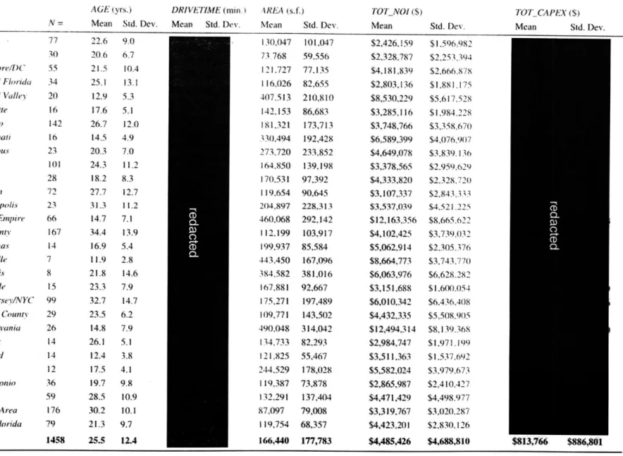
Each property is identified with a unique alphanumeric code and includes a variety of property-level data. Not all data is available for every property. Our unadjusted data set contains 4575 property codes, and includes quarterly financial information for a 6.25-year observation period that stretches from January of 2012 to March of 2018. We filter the data set in the following way. First, we exclude properties for which complete capex and NOI data is not available throughout the entire observation period. Next, we exclude properties whose total building areas have changed by more than 200 square feet during the period. We assume that smaller variations are essentially rounding errors that do not substantially affect the buildings' values, but that larger ones indicate additions or partial demolitions that could bias our results. We eliminate several properties whose building ages are not recorded. We are left with only one property in the San Diego MSA, so we eliminate it as well. The final sample consists of 1458 properties for which a total of 36,450 quarterly capex and NOI entries are available during the observation period. Table 4-1 contains descriptive statistics for both the overall sample and the individual MSAs. The average building in the sample has an area of approximately 166,000 square feet, is approximately 26 years old, and is about

redacted

Figures 4-1 through 4-5 are histograms that plot each of these variables' distributions in the sample. We observe that AGE and DRIVETIME are more or less normally distributed, but that the TOTNOI

and TOTCAPEX distributions are positively skewed, almost certainly because the AREA distribution

is also positively skewed. The standard deviations for these skewed variables are fairly large, because although most of properties are between 50,000 and 150,000 square feet, a substantial minority are considerably larger. Ghosh and Petrova (2017) note that this skewness also appears in their NCREIF data.

In this paper we classify New York/New Jersey, Baltimore/Washington DC, South Florida, Seattle, San Francisco, and Los Angeles as top markets. This generally follows academic and industry practice, as these markets tend to be the country's most supply-constrained and tend to provide the highest rents. Boston is often included in this category, but Prologis does not have a major presence in the Boston area, and no Massachusetts properties appear in our sample. It is also common to classify Chicago as a top U.S. real estate market, but the Chicago industrial buildings in our sample generate much less NOI per square foot than buildings in the markets listed above.

Figure 4-6 is a bar chart that shows our sample's property count by MSA. We observe that the properties tend to be concentrated in top markets, although Chicago, Dallas, Atlanta, Houston, and California's Inland Empire are also well represented. These latter MSAs provide access to major population and business centers, but apart from Chicago, they are inland and generally less supply-constrained. Demand increases in these markets tend to generate new development rather than increased rents.

Figure 4-7 shows the top markets that generate the highest average NOI per square foot. Orange County is actually the highest NOI generator in the country, but it is part of the Los Angeles metropolitan area and adjoins the ports of Long Beach and Los Angeles, the two busiest container ports in the United States. The Orange County buildings in our sample are also substantially newer, on average, than the Los Angeles County buildings (23.5 years old versus 34.4 years old). Generally speaking, the buildings in the top markets, including Orange County, are smaller (118,000 square feet versus 207,000 square feet) and older (29.4 years old versus 22.1 years old) than buildings in the other markets.

Finally, we observe that we have quarterly assessed values for 475 of the 1458 properties in our sample. Prologis obtains quarterly assessments only for properties that are held in the funds that it manages, and NCREIF collects data from these fund properties. Thus we estimate that about 33% of the properties in our sample have appeared in other academic capex papers that used NCREIF data.

Table 4-1 Final Sample Descriptive Statistics

AGE (yrs.) DRIVETIME (mini AREA (sIf.) TOTNOl (s)$

MSA N Mean Sid. Dcv. Mean Std. Dcv. Mean Std. Dev. Mean std. Dev.

Atlanta - 77 22.6 9.0 130,047 101,047 $2,426,159 $1.596;982 Austin 30 20.6 6.7 73.768 59.556 $2,328.787 $2,253,394 Balimore/DC 55 21,5 10.4 121.727 77.135 $4,181,839 $2.606.878 Central Florida 34 25.1 13.1 116,026 82.655 $2,803,136 81,881,175 Central Valley 20 12.9 5.3 407,513 210,810 $8,530,229 $5.617,528 charlotte 16 17.6 5.1 142,153 86.683 $3,285,116 $1.984.228 Chicago 142 26.7 12.0 181.321 173.713 $3,748,766 $3,358.670 Cincinnati 16 14.5 4.9 330.494 192,428 $6,589,399 $4,076,907 Columbus 23 20.3 7.0 _{273,720 233,852 $4,649,078 $3.839.136} Dallas 101 24.3 112 164,850 139,198 $3,378,565 82.959.629 0- Denver 28 18.2 8.3 _{170,531 97,392 $4,333,820 $2,328,720} Houston 72 27.7 12.7 119,654 90.645 $3,107,337 $2,843.333 (D Indianapolis 23 31.3 11.2 204,897 228,313 $3,537,039 $4.521 ,225 Inland Empire 66 14.7 7-1 0 460.068 292.142 $12,163.356 $8,665,622 LA County 167 34.4 13.9 _I 12,199 103,917 $4,102,425 $3,739.032 Las Ve rVas 14 16.9 5.4 0 199,937 85.584 $5,062.914 $2,305,376 Louisville 7 11.9 2.8 443.,450 167,096 $8,664,773 $3,743,770 Memphis 8 21.8 14.6 384,582 381,016 $6,063,976 $6,628,282 Nashville 15 23.3 7.9 167,881 92.667 $3,151,688 $1.600.054 New Jersey/NYC 99 32.7 14.7 175,271 197,489 $6,010,342 $6.436,408 Orange County 29 23.5 6.2 109,771 143,502 $4,432.335 $5,508,905 Pennsylvania 26 14.8 7.9 490.048 314,042 $12,494,314 $8,139.368 Phoenix 14 26.1 5.1 134733 82,293 $2,984,747 $1,971.199 Portland 14 12.4 3.8 121.825 55,467 $3,511,363 $1.537,692 Reno 12 17.5 4.1 244.529 178,028 $5,582.024 $3,979,673 San Antonio 36 19.7 9.8 11.387 73,878 $2,865,987 $2,410.427 Seatle 59 28.5 10.9 131,291 137,404 $4,471,429 $4,498.977 SF Hav Area 176 30.2 10.1 87,097 79,008 $3,319,767 $3,020.287 South Florida 79 21.3 9.7 119,754 68,357 $4,423,201 $2,830,126 Total 1458 25.5 12,4 166,440 177,783 $4,485,426 $4,688,810 00 TOTCAPEX ($) Mean Std. Dv $813,766 $886,801 This table presents descriptive statistics for 1458 properties and 36,450 quarterly capex and NOI observations during the period that stretches from January 2012 to March 2018. AGE represents the average building age during the observation period. DRIVETIME represents the round-trip travel time between the property and the center of the nearest MSA. SF is the building area, and TOT_,NOI and TOTCAPEX are the total NOI and capex over the duration of the observation period.

Building Age

-

Drivetime

50

.X

5~~

V, edce

Figure 4-2 Rownd Trip Travel Time to City Center in Minutes

0 >4 CD 0- -t CD C,, 0- C C,, CD tri Cd, CDI Number of Properties rF, 250k1 (250k, 500k] (500k, 750kJ (750k, IOOkl (I.000k, I,250kl o(1,250k. 1.500k] f-(1,500k, t,750kJ -(1.750k,m,0Xkj C (2.000k,

-250kl

to

-

.

04

-o'H

U

_0.

Number of Propenies CD [0, 1,500kl CD 4 (1.500k, 3,0(kJ (3,000k, 4,500k] (4,500k, 6,000k-CD (6,000k, 7,500k] (7,500k. 9,000kl

z

lk-Darker bars indicate Top 7 markets

SF Bay Area L.A County Chicago Dallas New Jersey/New York South Florida Atlanta Houston Inland Empire Seattle Baltimore/DC San Antonio Central Florida Austin Orange County Denver Pennsylvania Indianapolis Columbus Central Valley Cincinnati Charlotte Nashville Portland Phoenix Las Vegas Reno Memphis Louisville 176 142 101 167 79 77 59 66 72 55 36 34 30 29 28 26 23 23 20 16 16 15 - 14 14 12 Sm 7 0 20 40 60 80 100 120 Number of Properties Figure 4-6

Annual NOI/s.f. by MSA

140 160 ISO 200

Darker bars indicate Top 7 markets Orange County

SF Bay Area South Florida LA County Baltimore/DC New Jersey/New York Seattle Austin Portland Inland Empire Houston Pennsylvania Denver Las Vegas W Central Florida San Antonio Charlotte Reno Phoenix Central Valley Chicago Dallas Cincinnati Louisville Nashville Atlanta Indianapolis Columbus Memphis $0 $1 $2 Annual NOt/s.f. Figure 4-7 $3 $4 $5 $6 $7

Property Count by MSA

5. Results and Commentary

In this section we review the empirical results for the predictor variables in each of the regressions and graph the significant results. We expand on our findings with commentary from Prologis professionals. We do the same for the complete regression models, and then combine the results by examining capex as a fraction of NOI. The section ends with comments on industrial real estate depreciation. The complete regression results are presented in Appendix A.

5.1. Building Age

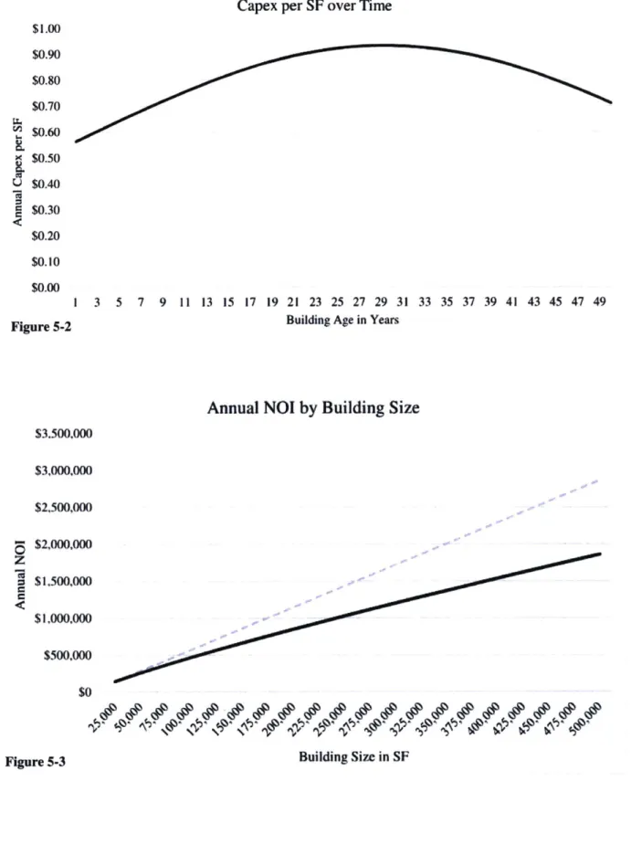
Our AGE and AGESQ results are largely as we expected, and each of the two variable coefficients is highly significant in each regression. In the NOI regression, the AGE coefficient is negative and the AGESQ coefficient is positive, indicating a continuous but decelerating NOI decline in real terms as a building ages, as shown in Figure 5-1. The signs of the coefficients are reversed in the capex regression, indicating that capex rises until it peaks when the building is about 30 years old. It then levels off and declines somewhat. This behavior is graphed in Figure 5-2.

Prologis professionals agreed that NOI typically declines with age. One professional observed that the decline is largely a result of functional, rather than physical, obsolescence. Shipping and manufacturing technologies have changed over time, and buildings that were state of the art decades ago are often poorly suited for modern uses. Older buildings tend to have non-standard loading dock sizes, low interior clear heights, and inadequate truck parking and maneuvering space. He stated that older buildings do not actually rent at a discount to new buildings if they are just as functional as the new buildings.

Regarding capex, the professionals observed that some of major property components have predictable lifespans. Roof and parking lot replacements are perhaps the largest line items that every property faces, and tend to come every 25 to 30 years. Sprinkler and HVAC system replacements are

not required in every property, but tend to be costly and are more frequent in older buildings. 5.2 Proximity to CBD

The DRIVETIME variable coefficient is not statistically significant in either of the regressions. We

investigated other versions of this variable in previous regressions that are not included in this paper. In one, we controlled for the difference in average travel times between MSAs by dividing each property's specific DRIVETIME value with the average value for the properties in that MSA. This

"standardized drivetime" value was measure of the property' proximity to the CBD relative to others in its market. In another version of the regressions, we split the DRIVETIME variable into two variables to see whether travel time has a systematically different effect in the top markets than it has in other markets. Neither of these approaches had statistically significant results.

Prologis professionals agreed that proximity to the CBD does not necessarily drive industrial rents. One observed that markets tend to have desirable areas that achieve higher rents, but that their desirability is the result of factors specific to individual markets that would not necessarily be important in other markets. He suggested that more general rent-increasing factors might be proximity to airports and proximity to high-income population centers. Another professional observed that many industrial tenants are manufacturers, and that these companies often draw their workforces from well outside urban cores. A facility too close to the city center might be difficult for them to staff. This observation validates the industrial rent model presented by DiPasquale and Wheaton (1996).

Callahan (2017) uses land transaction data to explore factors that drive industrial land values. He finds that proximity to CBDs results in higher industrial land prices, and suggest that this may be due to the reduced transport costs we described in our Research Methodology section. Alternatively, he notes that a higher land price may indicate an option premium in areas that are poised for redevelopment, and whose highest and best use may soon change from industrial to a more intense use. Our finding that proximity to CBDs is not associated with increased NOI suggests that the option premium effect explains higher land prices in those locations.

The Prologis professionals saw no reason that capex should vary between specific locations within a market. They observed that material costs are consistent from one location to the next, and that labor is mobile with a market. They did not find that tenants nearer to the city center had leverage to demand more tenant improvements or building improvements; rather, these costs are functions of the overall market and the condition of each property.

5.3. Building Size

The ln(SF) coefficient is highly significant in each regression. This was expected and is intuitively obvious, since a building's size clearly has an important impact on the rent it generates and the capex it absorbs. As we discussed in the Research Methodology section, the log-log models generate log(SF) coefficients that are elasticities, indicating the degree by which a building area change affects NOI and capex. The NOI regression's coefficient is approximately .86, indicating that a 100% increase in

24 Capital Expenditures in Industrial Real Estate

building size would generate an 86% increase in NOI. By contrast, the capex regression coefficient indicates that the same increase would generate only a 72% increase in that variable. Figures 5-3 and

5-4 graph annual NOI and capex as functions of building size. The dashed lines graph linear NOI and

capex growth with size, which would occur if there were no economies or diseconomies of scale affecting these variables. We observe that capex's growth is further from linear, meaning that capex economies of scale are more pronounced than NOI diseconomies of scale. Our models show that larger buildings have more efficient capex-to-NOI ratios.

Prologis professionals agreed that larger buildings require less capex per square foot, and described a variety of ways in which size increases efficiency. They noted that an engineer who produces construction documents for a roof replacement will charge little, if anything, more for a 200,000 square foot building than for a building half that size. Contractors' general conditions costs follow a similar pattern, and scale also increases buying power.

One professional observed that larger buildings tend to have longer lease durations, which reduces capex that occurs at lease transitions. This is consistent with Ghosh and Petrova (2017), who found that leasing commissions were the most important determinants of industrial capex.

5.4. Unused variables

Some earlier versions of our regressions contained additional predictor variables that are not included here. It is worth summarizing them briefly as they may prove useful in other studies.

We defined AVGVAL as the average assessed value of each property during the observation period. We have quarterly assessments only for the properties that are part of Prologis' funds, so including this variable reduces our sample size by two thirds. We log-transformed the variable so that we could more easily interpret the results.

We used STDCAP as a measure of the relative quality of individual properties. We calculated this variable in several steps. First, we divided average annual NOI by AVGVAL to determine each property's cap rate during the observation period. We then found the average cap rate for the properties in each MSA, and subtracted the market cap rate from the individual property cap rate to obtain

STDCAP. We assumed that negative STDCAP values indicated properties of higher than average

We found that the STDCAP coefficient was significant only at the p < .1 level. The ln(A VGVAL) coefficient was significant at the p < .001 level, but its inclusion caused the ln(SF) coefficient to become insignificant. Overall, the inclusion of these variables increased the capex regression's adjusted R2

value by about .05.

We chose not to incorporate these variables into the final version of this paper for several reasons. First, we do not have assessed values for most of the properties, and we did not want to dramatically reduce our sample size. Second, the STDCAP values incorporate NOI on the right side of the equations, which threatens to cause endogeneity in Equation 3-2, whose predictor variable is

TOTNO. Although these variables did not prove useful to us in this paper, they may be useful for

other researchers, particularly those using NCREIF data. The STDCAP and AVGVAL variables can generally be constructed for properties in the NCREIF database.

5.5. MSA Dummy Variables

We find that both NOI and capex are higher in top markets, but that the intensity of the effect is greater for NOI than for capex, which suggests that top markets have more efficient capex-to-NOI ratios. This observation does not account for the systematic differences in building stock between MSAs, though, which we discuss later in this section.

A Prologis professional suggested that capex variations between markets might be less than expected because their contractors are relatively mobile, even between distant locations. He stated that it is common for specialized contractors to travel halfway across the country to replace a roof on one of their buildings. While there are some additional costs associated with the travel, this practice tends to equalize construction costs across markets.

Figures 5-6 and 5-8 are bar charts that show the MSA effects on NOI and capex per square foot. We generate these results by applying the regression results to a hypothetical property whose size and distance to the CBD match the overall sample averages. This approach controls for building stock variations between MSAs, thus showing the pure market effects.

5.6. Model Fits

The adjusted R2

value for our NOI regression is approximately .85, which is unusually high for social science research. Our model explains 85% of the total NOI variation, indicating that industrial NOI is almost entirely a function of building size, building age, and market. This is an important

finding in its own right, and it gives us confidence that our capex fraction of NOI analysis is fairly accurate.

The capex regression has an adjusted R2 value of approximately .37. While it is lower than our NOI value, our R2 value is as high or higher than that in any previous capex regression that did not include property fixed effects. Still, the relatively low R2 suggests that the idiosyncratic variance described by Ghosh and Petrova (and implied in the low R2 results in other papers) remains at work in our data.

One Prologis professional suggested that a major portion of this variance may be due to leasing outcomes. Consider two properties in the same market whose size, age, and location are identical. Building A is leased to a manufacturing tenant who invests in major tenant improvements to fit out the building for its specific technical needs. After a few years the tenant files for bankruptcy or does not renew its lease, and the building reverts to the landlord. The professional estimated that it might cost $3.50 per foot to return this building to leasable condition, which is much higher than a normal TI allowance of perhaps $1.25 per foot for a new lease or $0.50 per foot at lease renewal. Building B, on the other hand, is leased to a tenant who renews the lease four or five times. These two buildings would absorb far different amounts of capex, despite being identical in all the variables included in our models. This topic is worthy of additional research.

5.7. Capex Fraction of NOI

We next combine our NOI and capex results to model capex as a fraction of NOI over time. We find this percentage for each building in the sample and average the results, and do the same for subsets of large buildings and small buildings. The typical building's value begins at 8%, rises to 22.5% after 35 years, and then declines to about 18% after 50 years. We observe that peak capex fraction of NOI lags peak capex by about 5 years. As a comparison of Figures 5-3 and 5-4 suggests, large buildings perform considerably better than small ones; the difference between buildings over 200,000 square feet and those under 100,000 is 4.6 percentage points on average over a 50-year period.

The regional effect on this variable requires more explanation, as we were faced with an apparent contradiction during our research. On one hand, a simple comparisons of asking rents and construction costs in each market suggests that top markets should have substantially lower capex fractions of NOI, since rents vary more widely than construction costs between markets. Prologis professionals predicted we would find this effect, and our regression results point to it as well.

On the other hand, it is common for academics and industry professionals to use broad rules of thumb when estimating this variable, without adjusting the value for top or lower-tier markets. Geltner et al. (2014), for example, state that capex tends to be 10-20% of NOI over the long term, and Prologis CEO Hamid Moghadam indicated that the number has historically been 12-15% in the industrial real estate business. And in fact it is not unreasonable to use such estimates, because actual capex fractions of NOI do not vary nearly as much between markets as the above factors suggest that they should. Figures 5-6 through 5-11 display the contradiction, but our descriptive statistics provide an explanation.

Figures 5-6, 5-8, and 5-10 apply our regression results. We use a theoretical property whose size matches the sample average (166,440 square feet), graphing the NOI, capex, and capex fraction of NOI it would generate in each market. We model the annual values for each variable and average them over a 50-year period. The bar charts display the average values, and include trend lines for easier interpretation. Top MSAs are shown in black.

The charts are sorted by NOI, and buildings in the top markets of course produce more than the others. The trend line is relatively steep, as the lower markets generate an average of 40% less per square foot than the top ones generate. Capex is also higher in top markets, but the difference is more subtle. These results reflect the market rent and construction cost disparities we discussed, and produce substantially lower capex fractions of NOI in the top markets.

Figures 5-7, 5-9, and 5-11 use our sample data. We simply total the annual NOI and capex per square foot produced by each market during the 25 quarters in our observation period. We observe that the NOI trend line in Figure 5-7 is similar to the line in 5-6, but the capex trend line is steeper, producing a capex fraction of NOI trend line that is completely flat. Clearly the capex values in top markets are higher than our regression values predict. The reason for this is obvious in the sample statistics: the buildings in top markets are considerably older and smaller than those in other markets, and as we describe in this section, old, small buildings absorb more capex than others. The average building in top markets is almost half the size of buildings in other markets (118,000 square feet compared with 207,000 square feet) and 7.3 years older (29.4 years old versus 22.1 years old). The bar charts show that the efficiency of the top markets is offset by the inefficiency of the actual building stock in those markets, producing capex fractions of NOI that are the same, on average, in top markets as in other markets.

Capital Expenditures in Industrial Real Estate 2828

5.8. Depreciation

Our findings lead to a broader observation about depreciation in industrial real estate. As we discussed in our Research Methodology section, Bokhari and Geltner (2016) found that net depreciation is essentially a function of NOI decline, as building values largely track NOI over the long term. To the extent that this is true, our graph of NOI over time is effectively a graph of net industrial depreciation, that is, depreciation over and above the cost of the capital improvements buildings absorb as their values decline. Adding the annual capex figures provides an estimate of gross depreciation. Figure 5-12 displays the results for our sample. The darker portion of the bars indicate year over year NOI declines, which we use as a proxy for property value declines. We estimate property value by applying a cap rate of 6.1 %, which is the average cap rate of all buildings in the subset of our sample with property value data. We can then determine annual capex as a percentage of property value, which is shown in the light bars. Combining the NOI decline (net depreciation) with annual capex yields gross depreciation. We observe that gross depreciation changes more gradually from year to year than either NOI or capex, as the high initial net depreciation is offset by low capex, and the low net depreciation later combines with higher capex. Annual gross depreciation drops slowly over time, starting at 3.1 % before declining to 2.7% by year 20 and 1.6% by year 40. We find that NOI declines are relatively minimal after this time, but we observe that NOI is only a proxy for property value to the extent that cap rates remain constant. Cap rate expansion with age would make net depreciation higher in later years, resulting in a more stable gross depreciation rate over time.

NOI per SF over Time

I Building Age in Years

F Igur

-Capital Expenditures in Industrial Real Estate 30

W- I

U

30 Capital Expenditures in Industrial Real Estate

Capex per SF over Time $1.00 $0.90 $0.80 $0.70 LT I E $0.60 S$0.50 U $0.40 S$0.30 $0.20 $0.10 $0.00 1 3 5 7 9 11 13 15 17 19 21 23 25 27 29 31 33 35 37 39 41 43 45 47 49

Figure 5-2 Building Age in Years

Annual NOI by Building Size

z