Publisher’s version / Version de l'éditeur:
Questions? Contact the NRC Publications Archive team at
[email protected]. If you wish to email the authors directly, please see the first page of the publication for their contact information.
https://publications-cnrc.canada.ca/fra/droits
L’accès à ce site Web et l’utilisation de son contenu sont assujettis aux conditions présentées dans le site LISEZ CES CONDITIONS ATTENTIVEMENT AVANT D’UTILISER CE SITE WEB.
2nd ACM Workshop on Embedded Sensing Systems for Energy-Efficiency in
Buildings (BuildSys 2010): 02 November 2010, Zurich, Switzerland [Proceedings],
pp. 13-18, 2010-11-02
READ THESE TERMS AND CONDITIONS CAREFULLY BEFORE USING THIS WEBSITE.
https://nrc-publications.canada.ca/eng/copyright
NRC Publications Archive Record / Notice des Archives des publications du CNRC : https://nrc-publications.canada.ca/eng/view/object/?id=65c7fdd7-c971-41e1-ba65-0fa3ff650f75 https://publications-cnrc.canada.ca/fra/voir/objet/?id=65c7fdd7-c971-41e1-ba65-0fa3ff650f75
NRC Publications Archive
Archives des publications du CNRC
This publication could be one of several versions: author’s original, accepted manuscript or the publisher’s version. / La version de cette publication peut être l’une des suivantes : la version prépublication de l’auteur, la version acceptée du manuscrit ou la version de l’éditeur.
Access and use of this website and the material on it are subject to the Terms and Conditions set forth at
Building-level occupancy data to improve ARIMA-based electricity use
forecasts
http://www.nrc-cnrc.gc.ca/irc
Building-le ve l oc c upa nc y da t a t o im prove ARI M A-ba se d e le c t ric it y
use fore c a st s
N R C C - 5 3 5 6 6
N e w s h a m , G . R . ; B i r t , B .
N o v e m b e r 2 0 1 0
A version of this document is published in / Une version de ce document se trouve dans:
2nd ACM Workshop on Embedded Sensing Systems for Energy-Efficiency in
Buildings (BuildSys 2010), Zurich, Switzerland, November 2, 2010, pp. 13-18
The material in this document is covered by the provisions of the Copyright Act, by Canadian laws, policies, regulations and international agreements. Such provisions serve to identify the information source and, in specific instances, to prohibit reproduction of materials without written permission. For more information visit http://laws.justice.gc.ca/en/showtdm/cs/C-42
Les renseignements dans ce document sont protégés par la Loi sur le droit d'auteur, par les lois, les politiques et les règlements du Canada et des accords internationaux. Ces dispositions permettent d'identifier la source de l'information et, dans certains cas, d'interdire la copie de documents sans permission écrite. Pour obtenir de plus amples renseignements : http://lois.justice.gc.ca/fr/showtdm/cs/C-42
Building-level Occupancy Data to Improve ARIMA-based
Electricity Use Forecasts
Guy R. Newsham
National Research Council Canada – Institute for Research in Construction 1200 Montreal Rd, M24, Ottawa Ontario, K1J 7X1, Canada +1 613 993 9607
[email protected]
Benjamin J. Birt
National Research Council Canada – Institute for Research in Construction 1200 Montreal Rd, M24, Ottawa Ontario, K1J 7X1, Canada +1 613 991-0939
[email protected]
ABSTRACT
The energy use of an office building is likely to correlate with the number of occupants, and thus knowing occupancy levels should improve energy use forecasts. To gather data related to total building occupancy, wireless sensors were installed in a three-storey building in eastern Ontario, Canada comprising laboratories and 81 individual work spaces. Contact closure sensors were placed on various doors, PIR motion sensors were placed in the main corridor on each floor, and a carbon-dioxide sensor was positioned in a circulation area. In addition, we collected data on the number of people who had logged in to the network on each day, network activity, electrical energy use (total building, and chilling plant only), and outdoor temperature. We developed an ARIMAX model to forecast the power demand of the building in which a measure of building occupancy was a significant independent variable and increased the model accuracy. The results are promising, and suggest that further work on a larger and more typical office building would be beneficial. If building operators have a tool that can accurately forecast the energy use of their building several hours ahead they can better respond to utility price signals, and play a fuller role in the coming Smart Grid.
Categories and Subject Descriptors
J.2 [Physical Sciences and Engineering]: Engineering
General Terms
Measurement, Experimentation, Human Factors
Keywords
Sensors, office buildings, occupancy, energy forecast
1. INTRODUCTION
Energy costs are rising, and there is a growing trend towards charging higher prices for energy when overall system demand is highest, in order to better reflect the true cost of generation, and to discourage on-peak use that might threaten grid stability. A building’s ability to reduce overall energy use and peak demand may be substantial, depending on the systems in place and data available to inform decisions, and tuning building power draw in response to utility signals and other inputs may be one element of the Smart Grid [1]. As part of this strategy a building operator may wish to explore and manipulate building energy use a few hours ahead; actions might involve load shedding, pre-cooling, charging of ice storage, activation of local generation, or a variety of other actions [2-6].
Building energy use data comprise a time series. In recent decades a class of time series analysis models named ARIMAX (Auto Regressive Integrated Moving Average with eXternal (or eXogenous) input) has been developed for forecasting in other domains, particularly in economics [7]. The “integrated” part of the name indicates that it is often required that one runs the analysis on the change in the dependent variable of interest (known as “differencing”), to render the series stationary1. “Auto regressive” indicates that the forecasted value of the dependent variable may be predicted from prior, known, values of the dependent variable. “Moving average” indicates that the forecasted value of the dependent variable may be predicted from prior values of the error term. “External input” refers to the optional use of independent predictors. The general notation for such a model is ARIMAX(p,d,q); if independent predictor variables are not employed then the notation is ARIMA only. The “p” indicates how far back in time one goes in using prior values of the variable of interest. For example, if the current value of a variable measured every hour is predicted using values of that
1
In a “stationary” series the values vary around an unchanging mean, and the variance over time is constant. Stationary series are a requirement for ARIMA models.
variable from one and two hours ago (known as “lag 1” and “lag 2”), p=2. Similarly, q refers to how many lags in the error term are used and “d” indicates how many times one takes the difference of the dependent variable. It is often the case that the variable of interest exhibits obvious periodic behaviour, generally referred to as “seasonal” behaviour. For example, building power use often displays a clear diurnal pattern; if one measures power hourly then there will be a seasonality of order 24. For modelling, one creates a new seasonal variable to reflect this variation, which is the current value of the dependent variable minus the value from one seasonal period ago. One can then apply differencing and lags to this variable and include these terms in the model. Thus the final general notation is ARIMAX(p,d,q)(P,D,Q)s, where P, D, and Q have the same meaning as above, but now refer to the seasonal variable, and s is the order of seasonality with respect to the measurement interval.
The most general mathematical form of the ARIMAX model equation is as follows [8]:
{Eq. 1}
,
wher
is the dependent time series e,
Yt
Xi,t is a set of i external predictor time series
at is a white noise time series representing random error, the values of this series are not known a
priori, but are an outcome of the iterative
parameter estimation methods used to generate the best-fitting model
t
µ is the mean of the series (=0 when series is
differenced)
indexes time
B is the backshift operator; i.e. BYt Yt‐; B Y Yt t‐ ; BB Yt B Yt
B is the autoregressive operator, a polynomial of order p in the backshift operator :
s B is, similarly, the seasonal autoregressive
operator, a polynomial of order P :
, ,
θ B is the moving average operator, a polynomial of order q in the backshift operator:
θs B is, similarly, the seasonal moving average
operator, a polynomial of order Q :
, ,
Ψi B is a transfer function for the effect of Xi,t o nYt :
, ,
δi B is the denominator polynomial in the backshift
operator, for the ith predictor:
, ,
δs,i B is similarly, the denominator seasonal
polynomial, for th ith predictor:e
, , , , ,
ωi B is the numerator polynomial in the backshift
operator, for e ith predictor: th
, , ,
ωs,i B is similarly, the numerator seasonal polynomial,
for th ith pe redictor:
, , , , , , ,
ki is the time delay for the effect of the ith predictor
(if the predictor cannot affect the dependent variable for a certain number of time steps for basic physical reasons)
ARIMAX models have been applied to building-related applications, including: modelling and forecasting of room temperature [9, 10], modelling of water and fuel use in a variety of buildings [11], optimizing the operation of cold storage in a large building [12], and forecasting and controlling the peak demand for electricity at a government complex [4].
Occupants are a key factor behind commercial building energy use, due to use of office equipment, lighting, plug loads, ventilation, thermal conditioning etc. Because ARIMAX models use prior values of the dependent variable, and because power use in a building is correlated with occupancy, the auto regressive and moving average components will implicitly carry the effect of occupancy. The question we explored was whether including an occupancy metric as an explicit independent variable would improve model accuracy. In [9] the authors suggested that variance in their ARIMA model of indoor temperature could be partially explained by variations in occupancy, and in [3] the authors lamented the lack of occupancy data for use in their artificial neural network model of building energy use.
In this study, our goal was not to compare ARIMA models to other forecasting techniques, but to use an
ARIMA model as a platform for exploring the added value of occupancy data. In certain buildings swipe card access can easily give building occupancy information, but where this is not used, are there other ways of determining how many people are in a building?
2. METHODS & PROCEDURES
The study was conducted in a three-storey building in eastern Ontario, Canada, comprising laboratories and 81 individual work spaces, and total serviced floor area of 5800 m2. Various wireless sensors were installed to collect data on activities related to occupancy, and other relevant information. Contact closure sensors were placed on the two exterior doors used as primary entrance and exit points, on two internal doors in common use, and on the refrigerator door in the main break room. PIR motion sensors were placed in the main corridor on each floor, and a carbon-dioxide sensor was positioned in a circulation area on the third floor. Wireless air temperature and horizontal illuminance sensors were positioned on the building’s roof to provide external climate data. These sensors were all based on the EnOcean platform. Repeater stations, with considerable trial-and-error experimentation in their placement, were required to deliver sensor data to the central receiver in a reliable manner. In addition, we collected data on the number of people who had logged in to the network on each day (but not when they logged off), network activity (bit transfer rates), and electrical energy use (total building, and chiller separately). Detailed information on the sensor system and data sources is available in [13].
2.1 Energy Use Forecasts Using ARIMAX
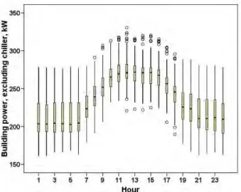
All variables used were hourly values (derived from measurements at shorter time scales). The dataset included weekdays only [12], because weekend occupancy was virtually nil and our long term interest was in peak demand load control.We subtracted chiller power from total building power. Thus the power variable included lighting, office equipment, lab equipment, and other plug loads that were likely directly related to occupancy, and thus perhaps of more relevance to the goals of this study2 (in [11] the authors suggested that non-weather related energy use would benefit from a separate analysis). Figure 1 shows the average hourly values of this power variable. The average peak load corresponds to ~46 W/m2, perhaps double the typical value for a building comprising offices only. An initial analysis suggested that network logins and motion sensor counts were likely to be the most
2
An earlier, linear regression time series analysis suggested that using total building power including the chiller yielded similar final results and conclusions.
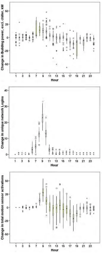
useful measures of occupancy ([13] provides information on all measures of occupancy, and the correlations between them). Analysis showed using once-differenced variables was appropriate for modelling purposes. Figure 2 shows average hourly values, and the expected rise (and fall) of building power draw coincident with the rise (and fall) of indicators of occupancy.
Figure 1. Average hourly values of total building power minus chiller. Length of box is interquartile
range (IQR); line in box is median; ‘o’ are outlier values more than 1.5 IQR from the end of the box; ‘*’ are outlier values more than 3 IQR from the end of the
box; whiskers show min. to max. range excluding outliers as defined above.
All analyses were conducted using the Forecasting module in SPSS version 18. Some SPSS routines require complete data sets, whereas we had some gaps in our data due to imperfect data collection systems and subsequent data cleaning. We had 79 days of complete and continuous data for building power draw; of these 79 days, 5 complete days of network login data and 17 complete days of motion sensor data were missing and were imputed with the mean of the non-missing values for that hour and day of the week.
Data were available from 1 am on June 12th, 2009 (Week 1 Day 1 Hour 1) to midnight on September 30th, 2009 (Week 17 Day 3 Hour 24). Initial model exploration was conducted on the majority of the dataset (Week 2 Day 1 Hour 1 to Week 16 Day 1 Hour 7), and checked for robustness on a split sample. Finally, the model was used to forecast power draw for the immediate future hours (Week 16 Day 1 Hour 8 onwards) and compared to the actual power draw data for this same period; i.e., data that were not used in the derivation of the model.
Figure 2. Average hourly values of the change in total building power minus chiller, unique network logins, and motion sensor activation (sum of three sensors).
3. RESULTS
Initially we derived a model for building power on the majority of the dataset without occupancy-related or other predictors. We did try cooling degree hours (base 18 °C, CDH18) for each hour (differenced) as a predictor to check for residual climate dependence. CDH18 was significant in the model but worsened the model fit. We therefore decided on the pure ARIMA model as the base model for comparison to later models. The automatically-generated, best fit model from SPSS Forecasting included a lag 7 term. However, this did not have any obvious physical explanation, and to keep the model compact we dropped this term from the model; this had only a tiny effect on the overall model fit. Therefore, the model was ARIMA(0,1,1)(0,1,1)24, and Eq. 1 simplifies to:
{Eq. 2}
,
The model parameters and fit statistics are shown in Table 1. For time-series data, stationary R-squared is a better measure of variance explained than simple R-squared, and higher values indicate a better fit. RMSE (Root Mean Square Error), MAPE (Mean Absolute Percentage Error), MAE (Mean Absolute Error), MaxAPE (Maximum Absolute Percentage Error), MaxAE (Maximum Absolute Error) are all measures where lower values indicate better performance. Normalized BIC (Bayesian Information) accounts for the number of parameters used in the model, and may penalize non-compact models; lower values indicate better model performance.
Table 1. Model with no external predictors, Week 2 Day 1 Hour 1 to Week 16 Day 1 Hour 7.
ARIMA Model Parameters MA (Power), θ MA (Power), Seasonal, θs, Lag 1 Lag 1 Estimate -.150 .753 SE .025 .017 t -5.908 43.377 Sig. .000 .000 Stationary R-squared 0.679 Normalized BIC 3.076 R-squared 0.984 RMSE 4.268 MAPE 1.244 MaxAPE 8.807 MAE 2.958 MaxAE 20.54
In the next step we added login data as a predictor in the model, using the Transfer Function option in SPSS Forecasting. Logins were significant in the model. The final model was ARIMAX(0,1,1)(0,1,1)24, and Eq. 1 thus simplifies to:
{Eq. 3}
,
The model parameters and fit statistics shown are shown in Table 2; fit statistics were generally improved compared to Table 1, albeit by relatively small amounts.
Table 2. Model with logins as predictor, Week 2 Day 1 Hour 1 to Week 16 Day 1 Hour 7.
ARIMA Model Parameters MA (Power), θ Seasonal, MA (Power), θs, Numerator (Logins), ω
Lag 1 Lag 1 Lag 0
Estimate -.150 .757 .100 SE .026 .017 .034 t -5.856 43.566 2.968 Sig. .000 .000 .003 Stationary R-squared 0.702 Normalized BIC 3.040 R-squared 0.985 RMSE 4.127 MAPE 1.217 MaxAPE 9.307 MAE 2.889 MaxAE 17.82
We tried adding motion sensor data as a predictor instead of logins, but this predictor was not statistically significant and did not improve the model.
We explored model robustness by specifying the model form in Table 2 to a split sample (Week 2 Day 1 Hour 1 to Week 10 Day 5 Hour 24; and, Week 11 Day 1 Hour 1 to Week 16 Day 5 Hour 24). All three model parameters from Table 2 were significant in both split samples, and the parameter estimates were similar.
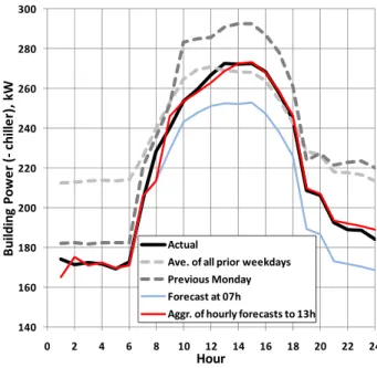
We then used the model from Table 2 to forecast building power into the future, using the methods in the SPSS Forecasting module. Note, that using the final model equation (Eq. 3), to forecast the value of Yt requires Xt . In this case, Xt is unknown a priori, and therefore it too must be forecast in some manner. This may be done with a separate ARIMA model for X alone [7]. The model in Table 2 was used in a forecast for the remainder of Week 16 Day 1 (a Monday). Figure 3 shows the forecast made at Hour 7 for the remainder of the day, and the actual building power. For comparison we chose two simple forecasts that might commonly be invoked: the average for all weekdays in the sample up to Week 15 Day 5; and the values from Week 15 Day 1 (the previous Monday). Beyond Hour 7 the ARIMAX model tends to under-predict the building power draw, forecasting a peak load 20 kW lower than the actual peak. The RMSE for Hours 8 to 24 are shown in Table 3.
Overall, the ARIMAX model performs better than assuming values from the previous Monday, but slightly worse that assuming average values from all weekdays.
Figure 3. Building power forecast using the ARIMAX model (at Hour 7, and hour-ahead forecasts to Hour 13), compared to: actual power;
average for all weekdays; the previous Monday.
It is common practice to update ARIMAX models as new data become available [12, 14]. We recalculated the model at every hour after Hour 7, and restricted ourselves to one-hour ahead forecasts; Figure 3 also shows the aggregate one-hour ahead forecasts up to Hour 13, and the forecast out to Hour 24 using the model updated at Hour 13. In this mode the RMSE is 73% lower than that from the average of all previous weekdays.
Table 3. Accuracy of forecasts for Hours 8 – 24 on Week 16 Day 1, for various methods
RMSE (Hours 8 – 24)
ARIMAX model (at 16.1.7) 17.4
ARIMAX model (aggr. to 16.1.13) 4.4
Average of all weekdays 16.3
Previous Monday 23.5
4. DISCUSSION
The improvement in the ARIMAX model with logins as a predictor was small but encouraging. There were several reasons why small effects might prevail in this building, and why we could expect a larger effect in a more typical office building. First, the study building had a high fraction of process loads for laboratory equipment, and a
140 160 180 200 220 240 260 280 300 0 2 4 6 8 10 12 14 16 18 20 22 2 B ui lding Po w e r (‐ ch ille r) , kW H 4 our Actual Ave. of all prior weekdays Previous Monday Forecast at 07h Aggr. of hourly forecasts to 13h
relatively lower fraction of loads related to the arrival and departure of occupants. This building was not unusual for its type, building power and occupancy profiles for a university computer science building [15] were very similar to those in our study building. In a building power profile for a more typical office building [3], the peak power draw was similar to our study building, but the overnight power draw was only 20% of this peak. Second, we expect that if logouts were also known in addition to logins, the model would be improved.
Motion sensor data did not improve our model. Perhaps this was because there was more variability in this parameter, or that it had less of a direct connection to occupancy than logins (i.e. logging in requires switching on a load, a computer, whereas activating a motion sensor does not). It might also simply be an artefact of the modelling process. Also, recall that a relatively large number of days of data were missing for this variable and had to be imputed, thus reducing the explanatory power. None of the other occupancy measures were effective in the model. Again, it would be interesting to explore whether such data streams were more effective in a more conventional office building. Further, the sensors and data streams we selected were a convenience sample from a wider possible range, other sensors might prove valuable (e.g. cameras, pressure sensors, noise data). Future development should explore robustness over longer time periods, through changing patterns of energy use throughout a year, and in a variety of building types.
5. ACKNOWLEDGEMENTS
We thank Loren Parfitt and Shawn Pedersen (Echoflex Solutions Inc.) for assistance with the wireless network. Richard Laurin, Mario Laniel and David Fothergill (NRC) provided IT support, and Kevin Li (NRC) helped access power meter data. Greg Nilsson (NRC) assisted with sensor calibration. We are also grateful to Ruth Rayman of NRC’s ICT Sector for financial and moral support.
6. REFERENCES
[1] Gershenfeld, N., Samouhos, S., and Nordman, B. 2010. Intelligent infrastructure for energy efficiency.
Science, 327 (Feb. 26th), 1086-1088.
[2] Zhou, Q., Wand, S., Xu, X., and Xiao, F. 2008. A grey-box model of next-day building thermal load prediction for energy-efficient control. International
Journal of Energy Research, 32, 1418-1431.
[3] Neto, A.H. and Fiorelli, F.A.S. 2008. Comparison between detailed model simulation and artificial neural network for forecasting building energy consumption. Energy and Buildings, 40, 2169-2176. [4] Hoffman, A.J. 1998. Peak demand control in
commercial buildings with target peak adjustment
based on load forecasting. Proceedings of the 1998
IEEE International Conference on Control Applications (Trieste, Italy), 1292-1296.
[5] Piette, M.A., Watson, D.S., Motegi, N., and Bourassa, N. 2005. Findings from the 2004 fully
automated demand response tests in large facilities.
Report for the PIER Demand Response Research Center. LBNL Report Number 58178. URL: http://drrc.lbl.gov/pubs/58178.pdf.
[6] Newsham, G.R. and Birt, B. 2010a. Demand- responsive lighting: a field study. Leukos, 6 (3), 203-225.
[7] Montgomery, D.C., Jennings, C.L., and Kulahci, M. 2008. Introduction to Time Series Analysis and
Forecasting. Wiley Series in Probability and
Statistics. John Wiley & Sons, Inc. (Hoboken, USA). [8] UC. 2010. Notation for ARIMA models. URL:
http://www.uc.edu/sashtml/ets/chap30/sect13.htm. [9] Loveday, D.L. and Craggs, C. 1993. Stochastic
modelling of temperatures for a full-scale occupied building zone subject to natural random influences.
Applied Energy, 45, 295-312.
[10] Rios-Moreno, G.J., Trejo-Perea, M., Castaneda-Miranda, R., Hernandez-Guzman, V.M., and Herrera-Ruiz, G. 2007. Modelling temperature in intelligent buildings by means of autoregressive models.
Automation in Construction, 16, 713-722.
[11] Lowry, G., Bianeyin, F.U., and Shah, N. 2007. Seasonal autoregressive modeling of water and fuel consumptions in buildings. Applied Energy, 84, 542-552.
[12] Kimabra, A., Kurosu, S., Endo, R., Kamimura, K., Matsuba, T., and Yamada, A. 1995. On-line prediction for load profile of an air-conditioning system. ASHRAE Transactions, 101 (2), 198-207. [13] Newsham, G.R. and Birt, B. 2010b. Detecting Total
Building Occupancy for More Efficient Operation,
National Research Council – Institute for Research in Construction, Research Report, RR-304. URL:
http://www.nrc-cnrc.gc.ca/obj/irc/doc/pubs/rr/rr304.pdf
[14] Kawashima, M., Dorgan, C.E., and Mitchell, J.W. 1995. Hourly thermal load prediction for the next 24 hours by ARIMA, EWMA, LR, and an Artificial Neural Network. ASHRAE Transactions, 101 (1), 186-200.
[15] Hay, S. and Rice, A. 2009. The case for apportionment. Proceedings of the First ACM
Workshop on Embedded Sensing Systems for Energy-Efficiency in Buildings (BuildSys 2009, Berkeley,