Publisher’s version / Version de l'éditeur:
Vous avez des questions? Nous pouvons vous aider. Pour communiquer directement avec un auteur, consultez la première page de la revue dans laquelle son article a été publié afin de trouver ses coordonnées. Si vous n’arrivez pas à les repérer, communiquez avec nous à PublicationsArchive-ArchivesPublications@nrc-cnrc.gc.ca.
Questions? Contact the NRC Publications Archive team at
PublicationsArchive-ArchivesPublications@nrc-cnrc.gc.ca. If you wish to email the authors directly, please see the first page of the publication for their contact information.
https://publications-cnrc.canada.ca/fra/droits
L’accès à ce site Web et l’utilisation de son contenu sont assujettis aux conditions présentées dans le site LISEZ CES CONDITIONS ATTENTIVEMENT AVANT D’UTILISER CE SITE WEB.
Applied Artificial Intelligence, 20, 1, pp. 1-33, 2006
READ THESE TERMS AND CONDITIONS CAREFULLY BEFORE USING THIS WEBSITE. https://nrc-publications.canada.ca/eng/copyright
NRC Publications Archive Record / Notice des Archives des publications du CNRC :
https://nrc-publications.canada.ca/eng/view/object/?id=2dbd6a74-1a51-4f64-8e48-fd1d7613f506 https://publications-cnrc.canada.ca/fra/voir/objet/?id=2dbd6a74-1a51-4f64-8e48-fd1d7613f506
Archives des publications du CNRC
This publication could be one of several versions: author’s original, accepted manuscript or the publisher’s version. / La version de cette publication peut être l’une des suivantes : la version prépublication de l’auteur, la version acceptée du manuscrit ou la version de l’éditeur.
For the publisher’s version, please access the DOI link below./ Pour consulter la version de l’éditeur, utilisez le lien DOI ci-dessous.
https://doi.org/10.1080/08839510500313711
Access and use of this website and the material on it are subject to the Terms and Conditions set forth at
Inferring and revising theories with confidence: analyzing bilingualism
in the 1901 Canadian census
Institute for
Information Technology
Institut de technologie de l'information
Inferring and Revising Theories with
Confidence:
Analyzing Bilingualism in the 1901
Canadian
Census*
Drummond, C., Matwin, S., and Gaffield, C.
2006
* published in: Proceedings of Applied Artificial Intelligence. 20(1) pp 1-33. 2006. NRC 47437.
Copyright 2006 by
National Research Council of Canada
Permission is granted to quote short excerpts and to reproduce figures and tables from this report, provided that the source of such material is fully acknowledged.
Analyzing Bilingualism in the 1901 Canadian
Census
Chris Drummond Chris.Drummond@nrc-cnrc.gc.ca Institute for Information Technology
National Research Council Canada Ottawa, Ontario, Canada, K1A 0R6
Stan Matwin stan@site.uottawa.ca
School of Information Technology and Engineering University of Ottawa
Ottawa, Ontario, Canada, K1N 6N5 and
Institute of Computer Science Polish Academy of Sciences
Warsaw, Poland
Chad Gaffield gaffield@uottawa.ca Institute of Canadian Studies
University of Ottawa
Ottawa, Ontario, Canada, K1N 6N5
Abstract
This paper shows how machine learning can help in analyzing and understanding historical change. Using data from the Canadian census of 1901, we discover the influences on bilingualism in Canada at be-ginning of the last century. The discovered theories partly agree with, and partly complement the existing views of historians on this ques-tion. Our approach, based around a decision tree, not only infers the-ories directly from data but also evaluates existing thethe-ories and revises them to improve their consistency with the data. One novel aspect of this work is the use of confidence intervals to determine which factors are both statistically and practically significant, and thus contribute appreciably to the overall accuracy of the theory. When inducing a decision tree directly from data, confidence intervals determine when new tests should be added. If an existing theory is being evaluated, confidence intervals also determine when old tests should be replaced or deleted to improve the theory. Our aim is to minimize the changes made to an existing theory to accommodate the new data. To this end, we propose a semantic measure of similarity between trees and demonstrate how this can be used to limit the changes made.
1
Introduction
This paper discusses a tool that can help in analyzing the increasing amount of available data and thus in understanding historical change. As such the work is a contribution to the field of historical methods. It is also a contribu-tion to artificial intelligence research not only as an interesting applicacontribu-tion of existing machine learning algorithms but also for the novel variants of these algorithms proposed to effectively deal with historical data. We view our work as a contribution in the important problem area of doing machine learning in the presence of domain knowledge. We show here how a human-built theory and the computer-constructed theory are combined, based on their validity on the domain data. In the same context of knowledge-based learning (to be contrasted with the recent statistically-oriented approaches), we present a principled tradeoff between comprehensibility and accuracy. In the opinion of many practitioners of machine learning and data mining, comprehensibility of the results is often the number one criterion of accept-ability of the results by their recipients (in our case, historians). It often outweighs more quantitative measures, e.g. accuracy on the hold-out set. We feel this is becoming more critical as data mining systems are used by more researchers in fields other than artificial intelligence to develop theories about their particular domains.
In this paper, we focus on exploring the influences on the languages spoken in Canada at the beginning of the last century. At the time of Confederation in 1867, language was a secondary issue to other concerns, most notably, religion. By the turn of the century, however, language was becoming an increasingly significant concern in Canada as in other western countries, and during the following decades, it came to be seen as a principal indicator of an individual’s identity. While much research has focused on the changing official views of language in Canada, little is known about the actual linguistic abilities of the Canadian population before the later twentieth century. Despite the central role that language has played in the origins of modern Canada, our current knowledge is limited to the political, religious and educational controversies that have erupted since the 1880s. In fact, this paper is the first study of bilingualism in Canada before 1971. As such, it serves as a point of departure for understanding the history of a key feature of the making of modern Canada
To address this problem, we apply a machine learning algorithm to the 1901 Canadian census. For the first time, the census asked all residents in Canada three language questions: mother-tongue, ability to speak English, and ability to speak French. Our research investigates a random five-percent sample of the 1901 enumeration that has been created by the Canadian Families Project. The sample is composed of all individuals living in house-holds that were randomly selected from each microfilm reel of the census enumeration for that year. Households were selected to permit analysis of individuals with relevant social units. The resulting sample is a cluster sam-ple but given the nature and large size of the samsam-ple, the design effect is not a concern is this study. For a detailed analysis of this question, see Ornstein [2000]. The sample includes data on 231,909 individuals over the age of five, and it allows us to explore how factors such as ethnic origin, mother-tongue, place of birth and residence, age and sex influenced the frequency of bilingualism across Canada. We build upon research that focused on the interpretive implications of how the census questions were posed, and how the actual enumeration was undertaken [Gaffield, 2000]. We now focus on the responses to these questions written down by the census officials at the doorsteps of individuals and families across the country.
We are certainly interested in inferring theories directly from the data. But we are also interested in testing existing theories, such as those repre-senting the views of politicians of that era, to see if they are confirmed, or indeed contradicted, by the data. Confirmation, or contradiction, is likely to be a matter of degree and not all parts of the theory will be affected equally. It may be possible to reduce the contradiction and avoid abandoning the
theory altogether. One advantage of the approach discussed below is that it minimizes the amount a theory is changed to bring it into accordance with the data. This should help us not only evaluate an existing theory but also to identify any erroneous assumptions on which it was based.
The algorithm we use is a decision tree learner. Decision trees are im-portant representations that have been used extensively in machine learning research. They are easy to understand, even by non-specialists, and have been used by domain experts in many diverse applications including agri-culture and law [Murthy, 1998]. They have not been used extensively in the historical research community. In research on social and cultural change in Canada, the statistical tool of choice has been logistic regression [Baskerville and Sager, 1998, Darroch and Soltow, 1994]. But an important property of any learning algorithm “is that it not only produce accurate classifiers (within the limits of the data) but that it also provide insight and under-standing into the predictive structure of the data” [Breiman et al., 1984, authors’ italics]. We would argue that logistic regression fails in this regard and this is critical in historical research. Decision trees do provide such insight and when applied to the census data will help to identify interesting population subgroups whose linguistic abilities differed from the dominant group. Furthermore, recent empirical research [Perlich et al., 2003] indi-cates that when working with very large datasets (in millions of examples), decision trees perform better than logistic regression. Analyzing historical census data requires learning methods that achieve high performance on data sets of this order of magnitude.
In decision tree learning, as with other representations with many degrees of freedom, an important issue is over-fitting avoidance. A complex tree that fits the training data well typically has unnecessary structure that does not contribute to the accuracy of the tree and may even degrade it. As the number of examples increases so does the problem [Oates and Jensen, 1997]. Many different algorithms have been proposed for pruning away unnecessary structure [Murthy, 1998]. In this application, we also regard structure that results in only a small increase in accuracy as unnecessary. The new or modified trees are intended to be used by non-specialists, so comprehensibility is of paramount importance. Although accuracy on new data is the main way of determining the validity of a theory, a more complex theory with only a minor improvement in accuracy is unwarranted and the simpler theory would be preferred.
Some algorithms have a parameter that controls the amount of pruning. To make the trade-off between accuracy and tree size more principled, we use confidence intervals to prune the tree rather than one of these methods.
Confidence intervals are closely related to statistical significance tests which have been used for pruning by a number of researchers [Quinlan, 1986, Frank, 2000, Jensen, 1991]. In recent times significance tests have been subjected to increasing criticism [Harlow et al., 1997]. It has long been known that statistical significance and practical significance are not the same thing. Statistical significance tests give no indication of the size of the effect. Even very small effects will be statistically significant if there is a sufficiently large amount of data. Using confidence intervals allows the determination of not only a statistically significant improvement in the accuracy of the tree, but also to quantify the size of the improvement. A test then will only be added to the tree if the expected accuracy gained is sufficiently large to justify it. One way to evaluate an existing theory represented by a tree is to com-pare its accuracy to a tree grown directly from the data. If the difference is large the existing theory might be rejected. But even if a theory has relatively poor accuracy, a small change might improve its accuracy sub-stantially. It would seem sensible to only reject the theory completely if the changes required were also large. To quantify the size of a change, a mea-sure is needed of the difference between two theories. For decision trees, one measure might be the syntactic change in the form of tree, say the number of tests added or deleted. An alternative is a measure based on some notion of the semantics of a tree.
The semantic measure proposed here is based on viewing a decision tree as a particular labeling of the attribute space. Under this geometric view, the semantics of a tree is determined by how it would label all future in-stances. Trees with the same partitioning of the attribute space into classes would be equivalent semantically even though they might be syntactically different. The semantic difference between two trees can then be determined by the number of potential instances classified the same way. But even this does not seem to capture the full semantics of a decision tree designed by an expert. Not only are semantics dependent on which attributes are chosen but also on the order in which they are chosen. Attributes that are closer to the root are likely to be considered more important in classifying the instances. To include these two semantic influences in decision tree learn-ing, we generate synthetic instances that are consistent with the expert’s tree designed to represent an existing theory. When modifying an expert’s tree, the performance of tests selected based on the synthetic data can be compared to the performance of tests selected based on some mixture of the synthetic data and new instances gathered from the domain. Using a mixture biases the system towards using attributes from the existing theory. Confidence intervals then determine when old attributes should be replaced
by new ones or deleted altogether to improve the theory.
This paper builds on previous work by the authors [Drummond et al., 2002]. Section 2.1 explores in greater depth the use of confidence intervals to prune decision trees and thereby control the trade-off between comprehensi-bility and accuracy. In Section 3, this technique is now applied not only to decision trees but also to probability estimation trees. It is shown that both types of tree are useful in identifying interesting population subgroups from the 1901 Canadian census data. Section 4 discusses in detail our semantic measure. It shows how the measure is combined with confidence intervals and new data to control the revision of an existing tree. Section 5 shows how this approach is used to evaluate and revise an existing theory on the influences on bilingualism in Canada in 1901.
2
Representing a Theory
Often in machine learning applications it is appropriate to represent the concept at more than one level of granularity, in order to abstract out the details unnecessary at a given level. For that reason, we use two types of tree to represent the theories. First is the standard decision, or classification, tree which divides the state space into regions which differ from their neighbors as to which class is the more common. Second is the probability estimation tree [Provost and Domingos, 2003] which typically makes finer distinctions. The neighboring regions need only differ significantly in the probabilities of belonging to each class. Both types of tree are interesting when exploring the census data. The first clearly identifies regions where bilingualism is dominant, the second identifies small subgroups where there are interesting differences in the probability of bilingualism. The standard decision tree is the one with which specialists and non-specialists, alike, have the most experience. There is also a clear consensus on how its performance should be measured. The probability estimation tree on the other hand, is much better at exposing historically interesting subgroups. Unfortunately there is no consensus on how to measure its performance, something we discuss in a later section.
Throughout this paper, we lay great emphasis on the understandability of the theories learned from the data. It is their explanatory power rather than their predictive performance that is of primary importance here. We are interested in the main influences on the languages spoken in Canada in 1901 and how these varied across different population subgroups. Good predictive performance matters only as a way of confirming the validity of
the explanations. As we argued in the introduction, we chose a decision tree algorithm for its comprehensibility. Many of the detailed choices about the way a decision tree is grown, and discussed in this section, have been motivated by this principle.
2.1 Growing A Tree
A binary tree is used to represent the theories induced from the data, the same representation used by the well known CART algorithm [Breiman et al., 1984]. The main advantage of a binary tree is that, unlike a tree with a greater branching factor, it only includes branches for attribute-values where the likelihood of classes is clearly different. We would argue that this is important for comprehensibility. If having French as one’s mother tongue is a good predictor of bilingualism, it does not mean that other mother tongues are worth distinguishing. Thus a binary tree helps us determine not only what are the important attributes but also the critical values of those attributes.
The tree is grown in the standard greedy manner, the best test, according a splitting criterion, is selected to be added to the tree. The main difference in our approach is that a test is actually added only when there is a high confidence that a worthwhile increase in accuracy will result.
f (a, v) = max
a,v |P (La,v|+) − P (La,v|−)| (1)
We use the splitting criterion proposed by Utgoff et al. [1997] and shown in equation 1. The continuous form of this criterion is a commonly used statistic, the Kolmogorov-Smirnov distance. The best split is the one with the greatest difference in the estimated probability of a positive instance going left P (La,v|+) and a negative instance going left P (La,v|−). The cri-terion is applied to each attribute and each value and the attribute-value with the greatest difference is selected. This value becomes the left branch of the split and the right branch represents the remaining values of the attribute. The difference in likelihood provides a measure of the probabil-ity that positive and negative examples come from different distributions. Likelihood difference is completely insensitive to the class distribution, but some research [Drummond and Holte, 2000] suggests this is an advantage rather than a disadvantage. A large difference tends to produce branches with a large difference in class ratios. Further splits should ultimately lead to better accuracy.
We could have used one of many splitting criteria proposed in the liter-ature [Murthy, 1998]. Two popular ones, information gain [Quinlan, 1993] and Gini [Breiman et al., 1984], both have a strong preference for generating branches that contain only a single class. When growing probability estima-tion trees, this biases the estimates towards extreme probabilities, zero and one [Zadrozny and Elkan, 2001]. The Kolmogorov-Smirnov distance based criterion does not have this tendency, so should be better for such trees. We could have used a different criterion for decision trees. However, by us-ing the Kolmogorov-Smirnov criterion, probability estimation trees are not completely different trees but rather expose more detail in already bilingual or unilingual majority regions. We feel this is more intuitive, particularly for non-specialists using the trees. Furthermore the Kolmogorov-Smirnov crite-rion, although prior insensitive, has a close relationship to accuracy which we exploit in generating a test statistic.
2.2 Choosing a Statistic
Our aim is to only add tests that improve the predictive performance of the tree by a useful amount. For decision trees accuracy is a good measure of performance, although there are reasons for not measuring it directly. But, accuracy is not a useful measure for probability estimation trees. Making a split where the majority class is the same on both branches does not improve accuracy, yet is still useful in identifying interesting subgroups. In this section, we propose a statistic which is a linear combination of likelihood difference and accuracy. One set of weights is useful for decision trees, another for probability estimation trees.
When growing a decision tree, accuracy is not measured directly as often adding a single test does not improve it at all; tests on multiple attributes are needed. We need a measure which is correlated with accuracy but will not suffer from this problem. We could use chi-square or indeed the difference in likelihood that we use as a splitting criterion. Other measures used as splitting criteria such as information gain are also potential candidates. For this application, the fact that these measures nearly always improve with additional tests is a disadvantage. When testing an existing theory, we also want to determine if removing tests is likely to improve accuracy. As a compromise, we use a measure based on accuracy but with a modified class distribution. Accuracy often does not improve when a test is added due to the strong imbalance in classes away from the root node. Reducing this imbalance means the measure is more likely to show improvement when a single test is added but also produces negative values.
To meet the necessary independence assumptions, our statistic is applied to separate pruning data [Jensen, 1991]. A pruning set is produced from a random 25% of the training set. The test chosen by the splitting criterion partitions this data, producing a contingency table as shown in Figure 1. The rows represent the class of the instances. Looking at the numbers not in parentheses, there are 32 positive and 8 negative examples, for a total of 40 instances. The columns show the number of instances going to the left, 26, and right, 14. If each side is labeled according to the majority class, there is no increase in accuracy. Yet, more of the positives go to the left and more of the negatives to the right which seems desirable. If the number of positives and negatives was closer to equality, say 24 and 16 as indicated by the numbers in parentheses, the sides of the split would be labeled differently and there would be an increase in accuracy.
2
6
(4)
(16)
Neg
Pos
Left Right
(18)
24
8
(6)
(12)
(24)
32
8
40
14
26
(22)
(18)
Figure 1: A Contingency Table
When applying the test statistic, a confusion matrix is produced from the contingency table. Based on the training data, the side of split where the positive likelihood is greater than the negative likelihood is labeled positive and the other side negative. Equation 2 gives the accuracy of the split if the left and right hand sides are labeled positive and negative respectively. Here, the role of the probability of each class, P (−) and P (+), is evident. To make a statistic less sensitive to class distribution, the values are replaced by ones closer to 0.5. If the terms are rearranged and the class probabilities set to 0.5, equation 3 results. This is essentially the difference between the likelihood functions of the two classes. This is very similar to our splitting criterion except that it is not the absolute difference in likelihood, it depends on how the sides of the split are labeled
Acc = P (L|+)P (+) + P (R|−)P (−) (2) = P (L|+)P (+) + (1 − P (L|−))P (−)
= P (−) + (P (L|+)P (+) − P (L|−)P (−))
= 0.5 ∗ (1 + P (L|+) − P (L|−)) (3)
A series of statistics can be produced by using equation 2 and applying the squashing function P′(a) = (P (a) + α)/(1 + 2α) to the class probabili-ties. Sensitivity to the class distribution is controlled by α. When growing decision trees, we use an α of one. This statistic can be viewed either as accuracy with a modified class distribution, or as the linear combination of two statistics, accuracy and likelihood difference. When growing probability estimation trees, we set both class probabilities to 0.5. The statistic is then just a measure of the difference in likelihood. In both cases, the statistic is divided by the fraction of instances reaching the test, and thus estimates the overall improvement in performance.
2.3 Pruning with Confidence Intervals
We use confidence intervals to determine when additional tree complexity is warranted by a worthwhile, and statistically significant, improvement in the predictive performance of the tree. This allows us to focus strongly on the issue of comprehensibility by preventing the extra structure often added to give marginal, even if statistically significant, improvement. Oates and Jensen [1997] show how standard decision trees continue to add structure even when there is no appreciable gain in accuracy.
Preventing additional structure is a form of pre-pruning. In the more commonly used post-pruning, the tree is first grown until it fits the training set well and then extraneous tests, not expected to improve accuracy, are pruned away. In pre-pruning, new tests are only added if they are likely to improve accuracy. Quinlan [1986] proposed using a chi-square significance test to pre-prune the tree. If the result of adding a new test is not statistically significant then noise might account for any apparent gain in using the test. Such a test is unlikely to generalize well. In C4.5, Quinlan [1993] adopted a post-pruning technique. He argued that pre-pruning suffers from the horizon effect, measuring the gain of a single test is insufficient as multiple new tests are needed to improve accuracy. Frank [2000] experimentally compared the two techniques based on significance tests and showed there was little
performance difference. The horizon effect was not found to be a problem provided the significance value was chosen appropriately.
Frank [2000] also investigated pre-pruning using a non-parametric sig-nificance test, called a permutation test. The rejection region of the null hypothesis is estimated by generating new random samples based on the data. In this paper, pre-pruning is based on confidence intervals rather than significance tests. We use a technique called bootstrapping [Efron and Tibshirani, 1993] which has been used extensively to generate confidence intervals. We follow the basic procedure proposed by Margineantu and Di-etterich [2000], who used bootstrapping to generate confidence intervals for the expected difference in cost between two classifiers.
We are also interested in bounding the difference in performance between two classifiers. When growing a tree and when evaluating a theory, the two classifiers are the one with a test and the one without. In addition when evaluating a theory, the two classifiers are the one with a test based on a particular attribute and the one with a test based on another attribute. In both cases the rest of the tree is unchanged so we only need consider instances that reach the test. Let us begin with the situation of comparing tests based on different attributes. We need samples of confusion matrices for each test, but the matrices are not independent. The dependency is represented by a three dimensional matrix, as Margineantu and Dietterich [2000] proposed, generated using the pruning data. The matrix is split vertically into positive and negative classes. The columns represent the number of instances sent down each branch by the first classifier and the rows represent the same for the second classifier. The matrix is projected down to two dimensions by summing over the other classifier. By labeling according to the likelihoods, a confusion matrix for each classifier is produced.
We generate new 3-D matrices (2 X 2 X 2) by sampling the original matrix as if it is a 8-valued multinomial. We project down to form the two confusion matrices and record the difference between the test statistic applied to each table. When comparing a tree with a test to one without, we do not need the full 3-D structure. But for simplicity, we use the fact that no test is effectively the same as a test that sends all instances down one branch. We sample the 3-D matrix as before but certain cells are empty. In both situations, we apply our test statistic to 500 randomly generated matrices. After sorting the resulting values in ascending order, the fiftieth element will be the lower bound of a 90% one-sided confidence interval.
If this lower bound is greater than zero, we are confident that the gain is statistically significant. In Figure 2 a), H0 is the null hypothesis (indicated by the vertical continuous line) that the difference is less than or equal to
zero. H1 is the alternative hypothesis (indicated by the vertical dashed line) that adding the test improves accuracy. Not only is the lower bound (indicated by the dashed semi-circle) greater than H0, it is also greater than 0.5%. We can be confident that this test would improve the accuracy of the tree by 0.5%, so the test would be added. If the bound is smaller than the chosen percentage or smaller than H0, as shown in Figure 2 b), the test would not be added. When starting with an existing theory, we are also interested in deleting structure. Now when the test is included it must be unlikely to produce a positive difference. So applying the same test but using the upper bound, (the dashed semi-circle in Figure 2 c)), allows us to determine that we are confident that removing structure does not degrade performance.
a)
H0
H1
> 0.5%
H0
H1
b)
90% UB
c)
H1
H0
90% LB
Figure 2: Using Confidence Intervals for Pruning
The values used to decide when a test should be added, a performance increase of 0.5% at a confidence level of 90%, where chosen by the authors to represent a reasonable confidence in a useful increase in accuracy. Future work will investigate the effect of varying these values and changing the test statistic used to estimate the increase in accuracy.
2.4 Choosing Performance Measures
Although we have stressed the issue of comprehensibility, some measure of predictive performance is still necessary to validate the theories generated from the data. It is also needed to determine how well the algorithm has worked from a machine learning perspective. In particular, we need to know if structure was added only when it was necessary.
we can see what percentage of the instances are correctly classified, in this case as either unilingual or bilingual. This will not work for probability esti-mation trees where often the difference between instances is the probability of belonging to a class but the most probable class is still the same. For in-stance, we might have one subgroup of people of which 25% are bilingual as opposed to a typical value of say 10%. They are still predominately unilin-gual but it might be of interest that this subgroup has a higher percentage of bilingual speakers.
For measuring the overall performance of probability estimation trees, there is no clearly preferred metric such as accuracy. One measure popular in climatology for probabilistic forecasts is the Brier score. This is one of a number of measures used by Zadrozny and Elkan [2001] to assess the perfor-mance of probability estimators. The Brier score for two class problems can be written as in equation 4. It is the mean squared difference between the predicted probability of a positive instance, P (xi), and one or zero depend-ing if the actual label yi of the instance is positive or negative respectively. As the Brier score is a measure of error, the best possible score is zero. The worst score is strictly one, but even a random guess, P (xi) = 0.5, will give a score of 0.25. BrierScore = 1 n n X i (P (xi) − yi)2 (4)
We also use the Mann-Whitney-Wilcoxon statistic, shown in equation 5. This measure compares the rank of the positive and negative instances according to their probability estimates, pi and qj respectively. This is the probability that a randomly chosen positive example will rank higher than a randomly chosen negative one and is also equivalent to the area under the ROC curve [Hanley and McNeil, 1982]. Here values range from zero to one, with one being the best value. In this case a random guess gives a value of 0.5.
M ann − W hitney − W ilcoxon = k X i l X j I(pi, qj))2 (5) I(x, y) = 1, when x > y 1 2, when x = y 0, when x < y (6)
to machine learning researchers. Unfortunately, there is not the strong fa-miliarity with them as there is with accuracy. So it is much harder to judge whether or not the differences in performance they show are important in practice.
3
Theories Induced from Data
In the next two sections, we explore theories generated directly from the data, firstly for the whole of Canada and then for the different geographical regions within Canada. Then in the following section, we look at evaluating the effectiveness of the algorithm from a machine learning perspective.
We use eight attributes from the 1901 census data felt to be potentially relevant to the issue of bilingualism. These attributes were selected in light of contemporary public debate as well as of studies of bilingualism in Canada in recent decades. At the turn of the past century, politicians and journal-ists stressed the importance of birthplace and “origin” (later to be called ethnicity) in determining linguistic ability. Given the perceived importance of speaking English, particular attention was focused on those born outside Canada and on those with “French” origin. These attributes were often associated with the question of mother tongue that was understood at the time as a feature of one’s family background rather than as a result of indi-vidual childhood experience. While sociolinguistic studies of later twentieth century Canada have also used birthplace, ethnicity, and mother tongue in their analyses, they have developed more complex interpretations in which age, sex, literacy, and levels of urbanization have also been found to help explain patterns of bilingualism. Our suspicion is that such attributes may have been even more important in 1901 when even basic literacy was not universal and when roughly three individuals lived in rural areas for every two city dwellers.
3.1 Bilingualism in Canada in 1901
We begin by looking at theories that deal with Canada as a whole and start by using a decision tree to represent the theory. For our purposes, a good decision tree is a simple one that accurately predicts if an individual is bilingual or unilingual from a combination of attribute-values. New branches will only be added if the number of instances on each side of the split is greater than 10. Numbers less than 10 might belong to a single family or a related group and be therefore of little interest.
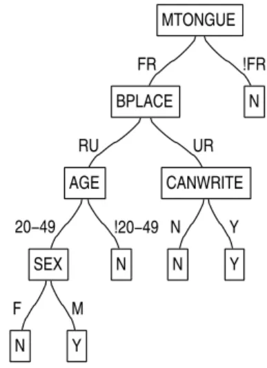
Figure 3 is the tree produced using the whole data set and represents the factors that affected bilingualism throughout Canada in 1901. To generate the class label Bilingual, we combined the attributes Can speak English and Can speak French but removed instances where one or both of the attributes were unknown. At each leaf the classification is shown: bilingual is labeled “Y” and unilingual (not bilingual) is labeled “N”. For the rest of this paper, unilingual will mean can speak French or English and bilingual will mean can speak both. In using this approach, it should be kept in mind, of course, that many other languages were spoken in Canada at this time despite the fact that the census questions only asked about French and English language ability. FR RU 20−49 F N M Y SEX !20−49 N AGE UR N N Y Y CANWRITE BPLACE !FR N MTONGUE
Figure 3: Decision Tree for Canada
The most important attribute, at the root of the tree, is mother-tongue. The split is between those that have French as their mother-tongue “FR”, and those that do not (divided into English, German, Gaelic and Others) “!FR”. Notably, for this latter category the tree terminates at a leaf imme-diately below the root. This classifies all people that do not have French as their mother-tongue as unilingual. The former category is further divided by birth place, those born in urban communities “UR” and can write are mostly bilingual. For rural communities “RU”, this is only true for males aged 20 to 49. This age attribute was originally continuous but was converted to a nominal one by dividing it into three intervals.
The decision tree in Figure 3 is in keeping with some, though not all, of the ways in which bilingualism was discussed in 1901 in Canada.
Politi-cians, journalists and other observers generally assumed that English was becoming the international language of commerce, and if Canada were to continue developing, everyone in the country should be able to speak it. In contrast, no public figure stressed the importance of learning French for eco-nomic reasons. The decision tree confirms that mother-tongue francophones accounted for most of the bilingualism in Canada. However, the tree also reveals considerable bilingual diversity within the francophone population in contrast to the characteristic inability of non-francophones to speak French. For mother-tongue francophones, their ability to also speak English appears to have related to their sex and age, ability to read and write, and whether they came from cities or the countryside. The general pattern that emerges suggests that, among francophones, individuals who were more likely to be involved in commerce were more bilingual as evident in the factors of literacy and birth place as well as age and sex.
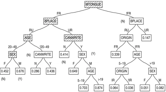
Figure 4 shows the probability estimation tree for Canada. Some of the upper part of the tree, indicated by the shaded nodes, is identical to the decision tree of Figure 3. There is additional structure which identifies sub-groups that differ in the proportion of bilingual individuals, but not in whether or not bilingual speakers are in the majority. The only difference in how these trees are grown is the test statistic used for pre-pruning, and dis-cussed at the end of section 2.2. The probability of being bilingual replaces the classification at each leaf.
FR RU 20−49 F 0.452 M 0.676 00 00 00 11 11 11 SEX !20−49 N 0.286 Y 0.436 CANWRITE 000 000 111 111AGE UR N 0.414 Y F 0.649 M 5−19 0.703 >19 0.874 AGE SEX 00000 00000 11111 11111CANWRITE 00000 00000 00000 11111 11111 11111 BPLACE !FR RU FR 0.339 !FR 5−19 IR 0.064 !IR 0.036 ORIGIN >19 F 0.051 M 0.082 SEX AGE ORIGIN (N) (Y) UR (N) (N) (Y) (N) 0.147 BPLACE 00000 00000 00000 11111 11111 11111 MTONGUE
The decision tree terminated in a leaf when the mother-tongue was not French. Some of the new attributes used on this branch are the same as those when the mother-tongue is French. Attributes such as birth place, sex, age are useful independent of the mother-tongue. Literacy, as indicated by the can write attribute, seems more important when the mother-tongue is French. Whereas ethnicity, particularly being of French origin (origin = “FR” as opposed to English, Irish, German, Scottish and others) seems more important when it is not. We also see that being of Irish origin “IR” increases the probability of being bilingual.
The probability estimation tree points to the importance of distinct lan-guage community sub-groups of the Canadian population some of which were the focus of public debate but most were not discussed. Overall, these trees make clear that both “English Canada” and “French Canada” were composed of quite different sub-groups. One intriguing result that deserves further study is the identification of a sub-group of Irish-origin bilingual children in Figure 4. Previous research has shown that census officials gen-erally attributed the father’s ethnic origin to children. It appears that these children are the result of linguistically-mixed marriages. The role of such marriages in fostering bilingualism during Canada’s formative decades was not emphasized at the time, and the extent of this pattern requires further investigation.
3.2 Regional Variance
We next explore how the factors that affected bilingualism varied across Canada. Figure 5 shows a map 1 of Canada in 1901 when the census was taken. One challenge in analyzing the data results from the uneven character of settlement across the country. The area that became known as the Prairies as well as the northern territories and districts were sparsely populated at this time, so we combine them into a single region, with a population size more in accordance with other regions. We also make a single region out of the eastern provinces; New Brunswick, Nova Scotia and PEI. We grow both decision trees and probability estimation trees for each of the regions. We combine them into single pictures, as we did in Figure 4, with the “decision subtree” indicated by shading the nodes.
For British Columbia, the decision tree classifies all mother-tongue fran-cophones as bilingual and all others as unilingual. A single node classifying everyone as unilingual would be very accurate due the large preponderance
Figure 5: Map of Canada in 1901 (N) FR (Y) N 0.017 Y 0.110 CANWRITE !FR 0.870 00000 00000 00000 11111 11111 11111 MTONGUE
Figure 6: British Columbia
of unilingual people in British Columbia, about 73%. But using the at-tribute mother-tongue correctly predicts over a third of the bilingual people without sacrificing much accuracy on the unilingual ones. Adding extra at-tributes produces no appreciable improvement in accuracy but the literacy attribute can write is added in probability estimation tree. This is used for individuals whose mother-tongue is not French. It is nearly seven times more likely that someone is bilingual if they can write. This goes against
the general trend in Canada where the literacy attributes seem to be only important when the mother-tongue is French.
FR N 0.421 Y 0.872 00000 00000 11111 11111CANREAD (N) (Y) (N) !FR 0.056 00000 00000 00000 11111 11111 11111 MTONGUE FR N 0.404 Y 0.848 !FR 5−19 >19 RU 0.026 0.063 (N) UR (N) (Y) 0.101 BPLACE AGE 00000 00000 00000 11111 11111 11111 MTONGUE 00000 00000 11111 11111CANWRITE
Figure 7: (a) Territories — (b) Manitoba
Certainly this is true for the Territories and Manitoba, Figures 7a and 7b. The former uses the attribute can read, the latter can write. In both cases, literate mother-tongue francophones are mostly bilingual. Surprisingly, the probability estimation tree adds no additional structure for the territories, no significantly different subgroups apparently remain. In Manitoba, for those whose mother-tongue is not French, people born in rural communities, particularly children, were even less likely to be bilingual.
(N) FR (Y) N 0.732 Y 0.902 CANWRITE !FR 5−19 FR 0.203 !FR RU 0.017 UR 0.030 BPLACE ORIGIN >19 RU FR 0.322 !FR 0.036 ORIGIN UR FR 0.423 !FR CB 0.066 IM 0.050 IMMIG ORIGIN BPLACE AGE 00000 00000 00000 11111 11111 11111 MTONGUE Figure 8: Ontario
In Ontario, see Figure 8, mother-tongue francophones again are predom-inately bilingual and, as shown by the probability estimation tree, literacy increases the probability of bilingualism. When the mother-tongue is not French, the adults born in towns are more likely to be bilingual and this probability is increased by being of French origin. We also see that immi-grants are slightly less likely to be bilingual.
(Y) (Y) (N) (N) FR N 0.026 Y 0.047 !FR 5−19 5−19 5−19 M M 0.686 0.298 0.507 0.732 F F 0.930 0.949 0.797 BPLACE >19 >19 >19 RU UR 000 000 111 111 000 000 111 111AGE AGE AGE SEX SEX 00000 00000 00000 11111 11111 11111 MTONGUE 00000 00000 00000 11111 11111 11111 CANWRITE Figure 9: East
For the Eastern provinces, Figure 9, the majority of literate adult mother-tongue francophones were bilingual. The probability estimation tree make further distinctions for those whose mother-tongue is French. Men tend to be almost all bilingual particularly if they are literate. Literate city-bred females are also almost all bilingual. For those whose mother-tongue is not French, adults are twice as likely as children to be bilingual.
For Quebec, Figure 10, a quite different decision tree is produced. Al-though the attribute mother-tongue is used, it appears much further down the tree, close to the leaves. The most important attribute is birth place, whether the person was born in a rural or urban community. The attribute mother-tongue has considerably less discriminatory power than birth place. The latter divides the population into two groups one which is predomi-nately bilingual and one unilingual, the former does not. The attributes used on both sides of the split based on birth place are very similar. How-ever, of people born in rural communities children are immediately classified as unilingual. The overall tree is much less accurate than those of the other regions. But as there was a nearly equal number of bilingual and unilingual speakers in Quebec, it still a considerable improvement over the majority
FR RU 20−49 F F F 0.273 M M M 0.321 !20−49 N N Y N N Y Y Y Y CANWRITE (N) (Y) (N) (N) (Y) (N) (N) (Y) (N) UR 0.133 0.451 0.323 0.640 >19 000 000 111 111 00 00 00 11 11 11 0.402 SEX 000000 000000 000000 111111 111111 111111 00000 00000 11111 11111 00000 00000 11111 11111 CANWRITE CANWRITE CANWRITE 00000 00000 11111 11111BPLACE !FR !FR !FR FR FR 0.198 0.345 5−19 5−19 0.658 0.544 0.871 >19 0.441 0.673 0000 0000 1111 1111 00000 00000 00000 11111 11111 11111 MTONGUE MTONGUE MTONGUE 000 000 111 111 0.628 SEX AGE SEX AGE AGE Figure 10: Quebec classifier.
The probability estimation tree for Quebec adds relatively little struc-ture. But it does show one interesting feature: for those born in urban communities the division for females and males is based on the same at-tributes in the same order, but the probabilities are lower for females. This suggests that the additional attributes are not highly context sensitive, i.e. largely independent of sex. For rural communities the order of attributes is different but again sex and literacy are strong predictors of bilingualism.
The regional decision trees reveal an extent of diversity in language pat-terns that goes well beyond the overall pattern for Canada. In addition, this diversity diverges considerably from the assumptions of the contempo-rary public debate. For the most part, for example, Quebec was assumed to be a quite homogeneous society especially in the countryside. The gen-eral picture was of a unilingual French-language rural world in Quebec that contrasted with the more bilingual urban communities of Montreal and to a lesser extent Quebec City. The decision trees reveal that Quebec was indeed a quite distinct part of Canada in terms of bilingualism but that within this distinction there was considerable diversity. Most strikingly, the importance of economic factors is seen in the greater tendency of middle-aged males in rural areas of Quebec (more likely to be working in rural industries or in the
forest economy) to be more bilingual
The probability estimation trees not only emphasize the considerable diversity that characterized linguistic patterns across the country but also suggest how the relationship between various factors operated differently in different contexts. For example, the influence of literacy on bilingualism is inconsistent much as sex does not always appear to relate to language patterns in the same way as illustrated by urban similarity but rural dis-similarity in Quebec. The general picture that emerges from the trees is that different factors explain levels of bilingualism in different regions of Canada and among various sub-groups. In other words, different parts of Canada did not contribute to the country’s overall diversity simply as a result of their different populations; rather, the same demographic and cul-tural groups tended to be bilingual or not depending on where they lived in Canada. Clearly, linguistic ability in early twentieth-century Canada re-flected complex factors that, themselves, played different roles in different settings. In contrast, public debate at the time (and a great deal of subse-quent scholarly analysis) tended to divide Canadian society into a few large components, most notably in terms of bilingualism, that of French Canada. While this focus is understandable as illustrated by the probability estima-tion trees’ attenestima-tion to those with French as a mother tongue, it is also clear that the question of bilingualism cannot be simply summarized in this way for Canada in 1901.
3.3 Measuring Performance
In the two previous sections, we were interested in what the trees could tell us about the factors that affected the propensity of bilingualism in Canada in 1901. In this section, we focus on the predictive performance of the trees both to support the conclusions we drew and to test if the algorithm worked as described in section 2. To get reliable results, we test performance on data not used to generate the trees, we kept back 25% of the instances for testing. The training and test sets are stratified to maintain the ratio of bilingual to unilingual speakers.
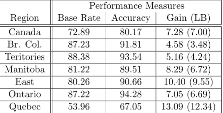
Table 1 shows the accuracy of each of the decision trees compared with the base rate performance. The first row is for Canada as a whole, the rest for its various geographical regions. The base rate is the accuracy obtained by predicting everyone is unilingual and is therefore the proportion of unilin-gual speakers in that region. Notably for all regions bar Quebec the base rate number is large from 80-90%, so it difficult to do better than predicting everyone is unilingual. But for these regions typically the remaining error is
nearly halved. So performance improvement is not only statistically signifi-cant but of sufficient size to be practically interesting. This goes some way towards supporting the conclusions drawn in previous sections, certainly some of the divisions made have predictive power. But it does not validate the presence of every division, an issue we discuss below.
Performance Measures
Region Base Rate Accuracy Gain (LB)
Canada 72.89 80.17 7.28 (7.00) Br. Col. 87.23 91.81 4.58 (3.48) Teritories 88.38 93.54 5.16 (4.24) Manitoba 81.22 89.51 8.29 (6.72) East 80.26 90.66 10.40 (9.55) Ontario 87.22 94.28 7.05 (6.69) Quebec 53.96 67.05 13.09 (12.34)
Table 1: Performance of Decision Trees
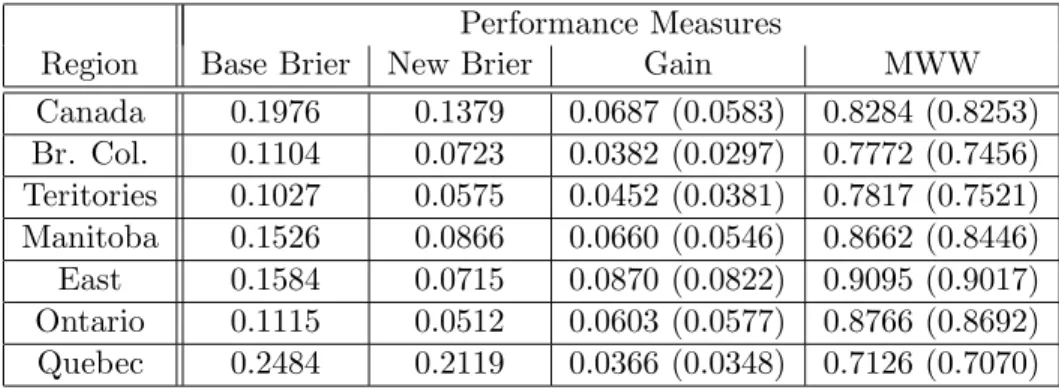
Table 2 shows the performance measures for the probability estimation trees. Here, the base rate for comparison is the Brier score when the prob-ability of being bilingual is set at the probprob-ability for the whole population of that region ignoring the attributes. Unfortunately, there is not the same intuitive feel for these numbers as there is with accuracy. But using a sim-ilar method to how we viewed the gain in accuracy, we can treat them as ratios to their base rates. Then for at least the territories, Manitoba, the Eastern provinces and Ontario there is a decrease in Brier score of one half. The base rate for the Mann-Whitney-Wilcoxon statistic is always 0.5, so subtracting 0.5 from the numbers in the last column of table 2 will give the gain. The gains here do at least roughly accord with those indicated by the Brier score. They agree that the largest gain is for Eastern provinces but notably they disagree on the second one. The Brier score prefers Ontario whereas the Mann-Whitney-Wilcoxon statistic chooses Canada as a whole. Further study would be needed to determine the exact reason for this.
Overall the trees showed meaningful improvement in predictive perfor-mance, but here we look at the contribution made by each attribute in the tree. Figure 11 shows the tree for Canada with numbers added, adjacent to each internal node (not a leaf), to indicate the performance gain achieved by adding that test. The shaded nodes, representing the “decision subtree”, have a number in parentheses for accuracy gain. All nodes have a number for the decrease in Brier score, multiplied by 100 to make it comparable to
Performance Measures
Region Base Brier New Brier Gain MWW
Canada 0.1976 0.1379 0.0687 (0.0583) 0.8284 (0.8253) Br. Col. 0.1104 0.0723 0.0382 (0.0297) 0.7772 (0.7456) Teritories 0.1027 0.0575 0.0452 (0.0381) 0.7817 (0.7521) Manitoba 0.1526 0.0866 0.0660 (0.0546) 0.8662 (0.8446) East 0.1584 0.0715 0.0870 (0.0822) 0.9095 (0.9017) Ontario 0.1115 0.0512 0.0603 (0.0577) 0.8766 (0.8692) Quebec 0.2484 0.2119 0.0366 (0.0348) 0.7126 (0.7070)
Table 2: Performance of Probability Estimation Trees accuracy. 0.452 0.676 00 00 00 11 11 11 SEX 0.286 0.436 CANWRITE 000 000 111 111AGE 0.077 0.047 0.011 UR 0.072 0.163(0.54) 0.081 0.185 (0.37) 0.246 (1.79) 0.362 (1.66) 4.613 (2.91) 0.108 0.005 0.001 0.414 Y F 0.649 0.703 0.874 AGE SEX 00000 00000 11111 11111CANWRITE 00000 00000 00000 11111 11111 11111 BPLACE 0.339 0.064 0.036 ORIGIN 0.051 0.082 SEX AGE ORIGIN 0.147 BPLACE 00000 00000 00000 11111 11111 11111 MTONGUE
Figure 11: Incremental Performance Gain
The root node contributes most to the overall accuracy of the tree. As we move down the tree additional tests contribute less, but still in excess of the 0.5 threshold we set. In fact, generally for the decision trees, attributes seem to be added if, and only if, they result in an increase in accuracy at the leaves of a practically significant amount. Although for the larger trees this is not always the case. This might be due to using a 90% confidence limit, 10% of the time this limit will not be met. It might also be due to the test statistic not being a direct measure of accuracy. In the latter case, post-pruning using accuracy might address the problem, but this remains
the subject of future work. For Quebec, it was possible to increase accuracy by about 0.7%, by reducing the confidence interval to 50% and removing the requirement for any gain. But to achieve this, the number tests went from 9 to 32 so is of debatable merit. With the test statistic we use, it is possible to produce a split where the majority class for each branch is the same. This makes no difference in accuracy and can be removed to make the tree smaller. In fact, for most of the trees this was unnecessary as no additional structure was added. The tree for Quebec had one extra test for mother-tongue being French and the Eastern provinces had one extra test for the individual’s sex.
Returning to Figure 11, the numbers for the decrease in scaled Brier score tend to change more rapidly than those for accuracy. As there are also many additional tests, the values close to the leaves are quite small. Thus whether or not the gain is achieved that is practically significant is not clear, although visual inspection of the differences between the probabilities at each leaf suggests useful distinctions are being made. The Brier score can be decomposed a number of different ways into various components. One such decomposition is discussed by Zadrozny and Elkan [2002]. We are really only interested in the component that represents the difference between the estimated and true probability, typically called calibration. The small gain achieved may be partly due to the other components. They tend to be larger when the true probabilities, and therefore even well calibrated estimates, are far from zero or one. Our alternative, the Mann-Whitney-Wilcoxon statistic, clearly shows a useful gain for the all the complete trees. We informally experimented with using this to measure the gain in adding each attribute. But the gain, particularly towards the leaves, was still small. Another disadvantage of this metric is that it does not directly measure good calibration rather it measures the relative ranking of positive and negative examples. Clearly neither measure gives the intuitive insight supplied by accuracy. So further work is needed to determine whether the small gain is due to our test statistic adding too much structure or is a consequence of the performance metric.
4
Revising an Existing Tree
In this section, we discuss how to revise an existing tree, such as one repre-senting the views of politicians in Canada in 1901, to agree with the available data. One might compare the tree with one grown directly from the data and modify it to reduce any apparent differences. However two quite
differ-ent theories might still have similar accuracy on the data. In fact, even a theory with relatively poor accuracy, might only require a small change to improve its accuracy substantially.
One way a tree might be modified to account for new data is the addi-tion of new branches. However, this would not remove existing unnecessary structure or reorder the importance of features in the model. Suppose that we believe that having a mother tongue of French is an important predic-tor of bilingualism. Perhaps, in fact, literacy represented by the attribute “can write” is the real predictor. Additional branches will show this depen-dence, the “Syntatic Change” in Figure 12, but the apparent dependence on mother tongue will remain. We would argue that the ability to reorder and ultimately to remove attributes, the “Semantic Change” in Figure 12, is important in changing the theory to reflect the data. This is why we have taken a particular view about the semantics of a theory and modified the decision tree algorithm to reflect this view.
FR FR N N N N Y N N Y Y Y N Y Y Y CANWRITE CANWRITE CANWRITE !FR !FR MTONGUE MTONGUE Change Syntactic Semantic Change
Figure 12: Semantic versus Syntactic Changes
This work has much in common with research concerned with theory revision [Mooney, 1993, Towell and Shavlik, 1994].The main difference lies in the use of a definition of the semantics of the tree to quantify changes to the theory. This allows us to substantially change the tree if the data warrants it but keep existing structure that is confirmed by the data.
4.1 Capturing A Tree’s Semantics
In this section, we propose a way of capturing the semantics of a theory represented by a decision tree. This becomes important when trying to assess what impact new data should have on an existing theory. It is after all the effect on the semantics of a theory that we want to quantify. Using
the syntactic change in a tree is an indirect way of measuring this. We felt a measure based on how a tree partitions the attribute space, that also takes into account the ordering of attributes, is a more direct semantic measure.
To capture the semantics based on how the tree partitions the attribute space, we generate instances consistent with the tree, reversing the normal process. The problem with directly converting a tree to data is the very size of attribute space. With no prior knowledge of the distribution of data, ex-cept for that directly represented in the existing tree, it would be necessary to generate instances covering the Cartesian product of the attribute values. To limit the number of instances, we generalize the notion of an instance so that the probability of an attribute having a particular value is specified. This is similar to the treatment of unknown values in C4.5 [Quinlan, 1993] except a uniform distribution is used. This is the most natural “neutral” choice [Madigan et al., 1995] when there is no knowledge of the distribu-tion of values. As in C4.5 when the attribute tested is not a single value, the instance is sent down multiple branches. By adding a weight to the instance we can simulate the effect of multiple examples without incurring the additional processing cost.
Our approach to producing an initial tree, representing a user’s insights, has much in common with prior elicitation in Bayesian analysis [Madigan et al., 1995]. In Bayesian analysis, an expert generates imaginary data which can be used to convert uninformed priors into more informed ones. In our approach, the user constructs a decision tree to classify a specified number of imaginary instances, say 1000. An example of what such a tree might look like is shown in Figure 13. It is based on the decision tree for Manitoba induced directly from the data and discussed in section 3. Each leaf is marked with the number of individuals from the original thousand that are bilingual and unilingual. For instance, when the mother-tongue is other than French, the number of unilingual individuals is 765 much larger than the number of bilingual individuals, just 52.
To generate instances consistent with the tree, each path through the tree is represented by as many instances as there are classes at the leaf. So six instances are needed to be able to regenerate this tree. Three are for the positive class, bilingual and three are for the negative class, unilingual. An instance following an upper branch has the probability of the attribute value associated with each specified test set to one. For the lower branch, the probability is a uniform distribution over the remaining values. Figure 14 shows the probability values for some of the attributes for the positive instances. The negative instances will be identical except for the weights shown at the bottom of Figure 14.
FR N N (25) Y (17) Y Y (120) N (21) CANWRITE !FR N (765) Y (52) MTONGUE
Figure 13: A Simple Domain Theory
MTONGUE
Instance1
Instance2
Wt = 120
Instance3
Wt = 52
AGE
CANWRITE
Wt = 17
Figure 14: The Positive Instances
The attribute mother-tongue has five possible values, indicated by the dashed rectangles. The first two instances travel down the topmost branch of the decision tree. They have the probability of the mother-tongue being French set to one, indicated by the bold continuous rectangle. The third instance, which travels down the bottommost branch, has the probability of the tongue being French set to zero and all other values of mother-tongue are set to a probability of one quarter. The first two instances travel different branches of the attribute can write. The first instance has a one for the “N” value, the second instance a one for the “Y” value. All unused attributes on a specific path, such as age, have a uniform distribution across all values.
Using these instances, it is now possible to change the order of the tests, or indeed to add a new test, and produce the same partition of the attribute
space into classes. Figure 15 shows the effect of changing the root node from mother-tongue to can write. The same number of instances are classified as bilingual and unilingual. The distribution on the center branch is the same, but the top and bottom most branches have changed. As these two branches are a mixture of instances where the majority class was unilingual, they still classify instances as unilingual.
N N (407) Y (43) Y FR Y (120) N (21) Oth N (382) Y (26) MTONGUE CANWRITE
Figure 15: Changing the Root Node
The topmost branch is made up of the first instance in Figure 14 plus half the third instance, as shown in Figure 16. The remaining half goes down the bottommost branch. The third instance had a uniform probability for can write. As this attribute is now the root node, this instance must be sent down both branches. This is achieved by making an additional copy of the instance. For the original instance, the probability of value “N” for can write is set to one, the same as the first instance. For the copy, the probability for value “Y” is set to one, the same as the second instance. As there are only two values, the weight for both instances is set to half the original weight. If there were more, the weight is the original weight times the fraction of values represented by the branch. The number of positive instances at the leaf is now (17+52/2) or 43. There is no longer a uniform distribution for the attribute mother-tongue, which was different for the first and third instances. The splitting criterion would choose this attribute as a possible additional test. This would not, however, change the classification of instances. A linear scan across the instances indicates that the classification will not change if new tests are added, so no split is made. To construct a tree representing a user’s intuitions, a single leaf node is first generated. The user then specifies the expected number of instances of each class. This leaf node can be converted to an internal node by selecting
Wt = 26
CANWRITE
MTONGUE
Instance3
Instance2
Wt = 120
+Instance1
Wt = 17
Instance3
Wt = 26
AGE
Figure 16: The Revised Instances
an attribute and one of its values. The system adds the selected test and generates two more leaf nodes. The user can again specify how the classes are distributed according to the test. To remove a test, the user selects an internal node converting it to a leaf. This is repeated until the user is satisfied with the structure of the tree. It is possible that the user’s ordering of the attributes is not consistent with the distribution of instances the user has specified. The tree can be re-grown according to the instances or the distribution can be changed. One advantage of using the difference in likelihood as a splitting criterion is that it is relatively easy to determine how the distribution of instances must be changed to maintain the structure of the tree. At present, any adjustment must be carried out by hand by changing the distribution of classes. In future work, we intend at least to semi-automate the process by showing the alternatives to the user who can decide how the tree should be modified.
4.2 Updating the Tree
To update the tree at each existing test, the splitting criterion is applied to a combination of the old data generated to be consistent with the tree and the new data. By only considering tests suggested by this combination, we aim to minimize the changes made to the existing theory to accommodate the new data. If the original theory preferred certain attributes, any changes to the theory will tend to use those attributes, rather than introducing new attributes, say by promoting them higher up the tree. New tests will only be
introduced if the new data has a strong preference for them. To achieve this, the splitting criterion is applied separately to the old and new data. The values returned are combined linearly to form a single value. The coefficients are determined by the number of instances, or weight, of the old data versus the number of new instances.
There are four possibilities that might occur. A new test might be added where the original tree had a leaf. The original test might be replaced by a different test. The original test might deleted altogether, or the old test maintained. To determine which takes place, confidence in the new best test is determined. If the original tree had a leaf at this node, a new test will be added to the tree if the lower bound of the confidence interval is greater than 0.5. This is the same as growing the tree directly from the data. If the new test is the same as the old test nothing will change. If the new test is different and its confidence interval exceeds the threshold it is compared to the new test. If the lower bound of the confidence interval for the difference exceeds the threshold, the test will be changed. If the new test does not exceed the threshold and the upper bound of the confidence interval on the difference does not include zero, the test is deleted.
The old and new data might also differ in how an instance should be classified at a leaf. A confidence interval can be used to decide which classi-fication should be used. Again a bootstrapping technique is used, this time based on just the binomial ratios. At the leaf we can use lower bound of accuracy directly rather than our test statistic.
5
Evaluating an Existing Theory
In this section, we present an experiment showing how the method discussed in section 4 uses data to evaluate and revise an existing theory. The the-ory has been developed from analyses of debate in the House of Commons and newspaper coverage of political discussion about the language questions posed in the 1901 census. For a comprehensive analysis of the political de-bate about language, see Gaffield [2000]. The decision tree representing the theory, see Figure 17, was designed to classify an imaginary 1000 people. The design exercise began by ranking attributes according to their importance in the debate. Then each branch of the tree was assigned some proportion of the 1000 people, indicated by the numbers in parentheses. Next, each at-tribute was considered for its influence on bilingualism, and the number of unilingual and bilingual individuals was assigned. Politicians certainly did not all agree on the importance of various factors and their perceived
influ-ence on reported bilingualism, and therefore the experimental parameters represent a distillation of somewhat divergent views.
Ethnic origin was assessed to be the most important attribute, only those of French origin were expected to be bilingual, most other individuals were expected to be unilingual. The next most important attribute was assessed to be birthplace, being urban born was more strongly associated with bilingualism than being rural born. Attributes sex, age and can write were then added in that order. Once the tree was constructed, synthetic instances were generated to be consistent with the tree. The proportions of the classes at the leaves, indicated by the “Y()” and “N()” in the figure, were then adjusted so that the ranking of attributes was maintained, as discussed at the end of section 4.1. The tree is reasonably accurate (78.960%), only 1.2% less accurate than the tree grown directly from the data (80.169%).
FR RU F N (65) Y (20) M 20−49 N N (15) Y (12) Y Y (25) N (20) CANWRITE !20−49 N (35) Y (20) AGE SEX UR F 20−49 N N (10) Y (8) Y Y (20) N (10) CANWRITE !20−49 N (20) Y (10) AGE M >=50 N N (10) Y (8) Y Y (12) N (10) CANWRITE <50 Y (50) N (20) AGE SEX BPLACE !FR N (550) Y (50) ORIGIN
Figure 17: The Politicians’ Theory
Figure 18 shows the politicians’ theory after being revised using the data for the whole of Canada. This revised theory is more accurate than the politicians’ theory. It has, indeed, an accuracy (80.204% lower bound 79.926%) indistinguishable from that for the decision tree grown directly
from the data (80.169%) and shown in Figure 3. The base of the tree is identical to the tree grown from the data. Much of the structure from the theory has been deleted, but quite a lot remains, indicated by the dashed shapes labeled“A” and “B” in figure 18.
The most significant change to the theory is the first test, mother-tongue replaces ethnic origin. We experimented by growing some of the decision trees from section 3.2 but forcing the first test to be ethnic origin and remov-ing mother-tongue. The remainremov-ing attributes were identical but the resultremov-ing trees were between 1% and 2% less accurate. This suggests that replacing ethnic origin with mother-tongue accounts for most of the improvement in the revised theory. The additional structure, indicated by the “A’s” in fig-ure 18, is the part of the politicians’ theory which was not deleted when the tree was revised. It identifies two bilingual groups for people whose mother-tongue is not French. Urban males (labeled “A1”) of French origin are predominantly bilingual, as are urban females (labeled “A2”) of French origin, aged 20 to 49 who can write. These groups were identified in the original theory and as the data very weakly supports this division they have not been deleted.
The additional structure, indicated by the “B’s”, is not supported by the data even weakly. It was not deleted, however, as the tests did not indicate a statistically significant increase in accuracy. This structure does not change the classification of the tree and so could easily be deleted. The attribute sex labeled “B1” in the figure was in the probability estimation tree for Canada and did make a useful distinction between class ratios but is not useful for classification. The attribute sex labeled “B2” has a probability of being bilingual for males of 0.499. As this is just less than 50%, all instances reaching this leaf are classified unilingual. If the classification is changed the accuracy improves very slightly to 80.024%, this is why our test did not delete it.
From an algorithmic perspective, it seems that attributes were modified and deleted when there was a clear advantage in doing so. But when the data did not support such deletion, the semantics of the original theory was maintained. From a historical perspective, the Canadian politicians of 1901 used mother-tongue to help clarify ambiguities among the labels used for ethnic groups; they did not see language as being a good identifier in and of itself. These theory revision experiments suggest that mother-tongue was more important that politicians believed at the time. But they were aware that times were changing, but probably not to the extent to which the data seems to suggest, and this led to addition of language questions to the census.