Asymptotically optimal path planning and surface reconstruction for inspection

(1)

Asymptotically Optimal Path Planning and

Surface Reconstruction for Inspection

O

by

OCT 16

201 Georgios Papadopoulos

_LIBRARIES

S.M., Massachusetts Institute of Technology (2010)

Diploma, National Technical University of Athens (2007)

Submitted to the Department of Mechanical Engineering

in partial fulfillment of the requirements for the degree of

Doctor of Philosophy at the Department of Mechanical Engineering

at the

MASSACHUSETTS INSTITUTE OF TECHNOLOGY

September 2014

@

Massachusetts Institute of Technology 2014. All rights reserved.

Signature redacted

A uthor ...

...

D'epartment of Mechanical Engineering

June 16, 2014

Certified by...

Signature redacted

Nicholas M. Patrikalakis

Kawasaki Professor of Engineering

Thesis Supervisor

Signature redacted

Accepted by ...

SigDavideE.

.d

David E. Hardt

Chairman, Department Committee on Graduate Students

Department of Mechanical Engineering

(2)

(3)

Asymptotically Optimal Path Planning and Surface Reconstruction for Inspection

by

Georgios Papadopoulos

Submitted to the Department of Mechanical Engineering on June 16, 2014, in partial fulfillment of the

requirements for the degree of

Doctor of Philosophy at the Department of Mechanical Engineering

Abstract

Motivated by inspection applications for marine structures, this thesis develops algo-rithms to enable their autonomous inspection. Two essential parts of the inspection problem are (1) path planning and (2) surface reconstruction. On the first problem, we develop a novel analysis of asymptotic optimality of control-space sampling path planning algorithms. This analysis demonstrated that asymptotically optimal path planning for any Lipschitz continuous dynamical system can be achieved by sam-pling the control space directly. We also determine theoretical convergence rates for this class of algorithms. These two contributions were also illustrated numerically via extensive simulation. Based on the above analysis, we developed a new inspec-tion planning algorithm, called Random Inspecinspec-tion Tree Algorithm (RITA). Given a perfect model of a structure, sensor specifications, robot dynamics, and an initial con-figuration of a robot, RITA computes the optimal inspection trajectory that observes all surface points on the structure. This algorithm uses of control-space sampling techniques to find admissible trajectories with decreasing cost. As the number of iterations increases, RITA converges to optimal control trajectories. A rich set of simulation results, motivated by inspection problems for marine structures, illustrate our methods. Data gathered from all different views of the structure are assembled to reconstruct a 3D model of the external surfaces of the structure of interest. Our work also involved field experimentation. We use off-the-shelf sensors and a robotic plat-form to scan marine structures above and below the waterline. Using such scanned data points, we reconstruct triangulated polyhedral surface models of marine struc-tures based on Poisson techniques. We have tested our system extensively in field experiments at sea. We present results on construction of various 3D surface models of marine structures, such as stationary jetties and slowly moving structures (floating platforms and boats). This work contributes to the autonomous inspection problem for structures and to the optimal path, inspection and task planning problems. Thesis Supervisor: Nicholas M. Patrikalakis

(4)

(5)

Acknowledgments

I would like to first thank my advisor, Prof. N. M. Patrikalakis, for his continuous

support and direction. He was always available to discuss ideas and has provided me with the necessary materials and guidance to successfully pursue my research. I also would like to express my appreciation to my thesis committee members Professors M.

S. Triantafyllou and F. S. Hover of MIT and Dr. H. Kurniawati (of the University of

Queensland, Australia and formerly of SMART

/

CENSAM of Singapore) for their

guidance and comments. Dr. Kurniawati has co-authored several publications with me and has always been willing to share ideas in robotics research and to provide important technical input.

I would also like to thank my S.M. thesis advisor, Prof. J. J. Leonard of MIT, for his support and direction during my first years at MIT and my undergraduate advisor, Prof. E. G. Papadopoulos (of the National Technical University of Athens, Greece), who introduced me to different aspects of robotics. I also wish to express special appreciation to Professors E. Frazzoli, S. Karaman, and T. P. Sapsis of MIT for useful technical discussions. Especially Prof. Karaman, as an expert in optimal sampling-based path planning, was always available to discuss topics of common interest.

Last but not least, I would like to thank my wife Tina and my parents for their support during the course of my studies.

This work was supported by the Singapore-MIT Alliance for Research and Tech-nology (SMART), Center for Environmental Sensing and Modeling (CENSAM).

(6)

(7)

5 Asymptotically Optimal Inspection Planning for Systems with Dif-ferential Constraints 109 5.1 Problem Definition ... 110 5.2 Proposed Algorithms ... 112 5.3 Analysis ... 115 5.3.1 Optimality of RITA ... 116 5.3.2 Completeness of RITA ... 117 5.4 Results ... 120 5.4.1 2D Workspace Results ... 121 5.4.2 TSP-Art-gallery ... 128 5.4.3 3D Workspaces ... 130 5.4.4 Implementation ... 137

(9)

5.5 Summary and Discussion ...

6 Robustness of Approximate Optimal Trajectories 6.1 Introduction ...

6.2 Deterministic Theoretical Bounds ... 6.3 Probabilistic Theoretical Bounds ...

6.4 Monte-Carlo Framework for General Trajectory Evaluation . . . .

6.5 Summary and Discussion . . . . 7 Conclusions and Future Work

7.1 Conclusions ... 7.1.1 Surface Reconstruction . 7.1.2- Path Planning . . . . 7.2 Contributions ... 7.3 Future Work ... 7.3.1 Path Planning ... 7.3.2 Inspection Planning. . . 7.3.3 Surface Reconstruction . 147 . . . . 147 . . . . 147 . . . . 148 . . . . 151 . . . . 153 . . . . 153 . . . . 154 . . . . 155

A Probability to Get at Least one Trajectory that is

Approximation of the Optimal Trajectory

e-close to Any

157

B Convergence Rate for the First Milestone for the Discrete System 161

137 139 140 141 142 144 145

(10)

(11)

List of Figures

1-1 Thunder Horse oil platform after the Hurricane Dennis in 2005 [15J. . 23

1-2 Diver inspecting a platform in the Gulf of Mexico; the picture is taken from "TheOceanCorporation" [1]. . . . . 24

1-3 An illustration of a TSP-art-gallery approach: In this example, even if

the observation points are chosen correctly the resulting trajectory is not close to optimal because the TSP algorithm computes the visiting order ignoring the obstacles. . . . . 25

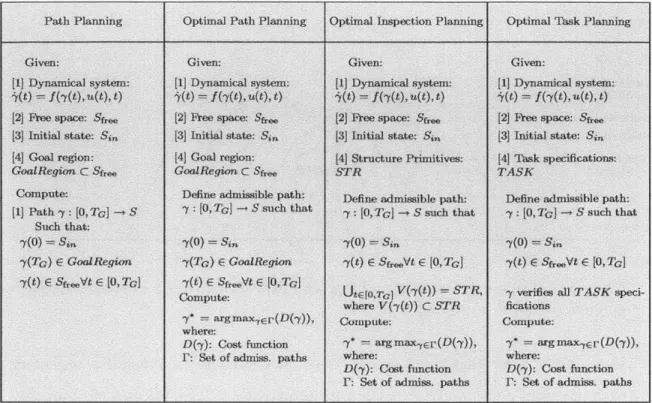
1-4 Different planning problems: the path planning problem, the optimal path planning problem, the optimal inspection planning problem and the optimal task planning problem. . . . . 27 1-5 The simple planning problem is a hard and a

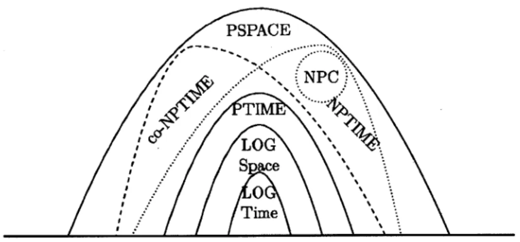
PSPACE-complete problem (adapted from [1001). . . . . 28

2-1 An illustration of greedy strategy that always chooses to move to a configuration within R radius from its current position, that can see the largest unseen structure. The environment contains two structures, i.e., the "U" shaped at the bottom and the line at the top. In this example, the greedy strategy may fluctuate moving down and up, while the shortest trajectory would move to cover the structure on the top

(12)

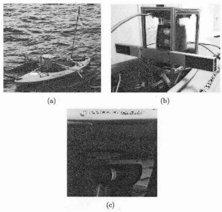
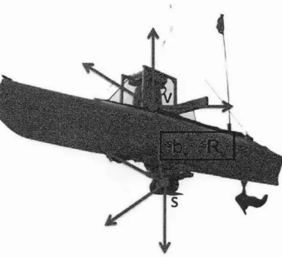
3-1 (a) The ASV with Velodyne LiDAR mounted on top of it. Two

pon-toons are attached to the ASV to improve its stability. (b) The Velo-dyne LiDAR and the mounting platform for placing the LiDAR in an inverted configuration on the ASV. (c) The BlueView MB2250 micro-bathymetry sonar is mounted in a sideways configuration. . . . . 49

3-2 The online map: we use big simplification cell size. . . . . 53 3-3 The off-line map: Less simplified data are used to get the vehicle's

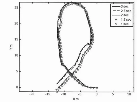
trajectory (a set of transformation matrices) and then the vehicles' trajectory is used to project raw data resulting in a dense point cloud. 54 3-4 Trajectories generated during the first 100 seconds of one of the

ex-periments: Trajectories corresponding to different At form a sequence with decreasing difference. . . . . 55 3-5 The coordinate systems of LiDAR and sonar. b, and 8R, denote the

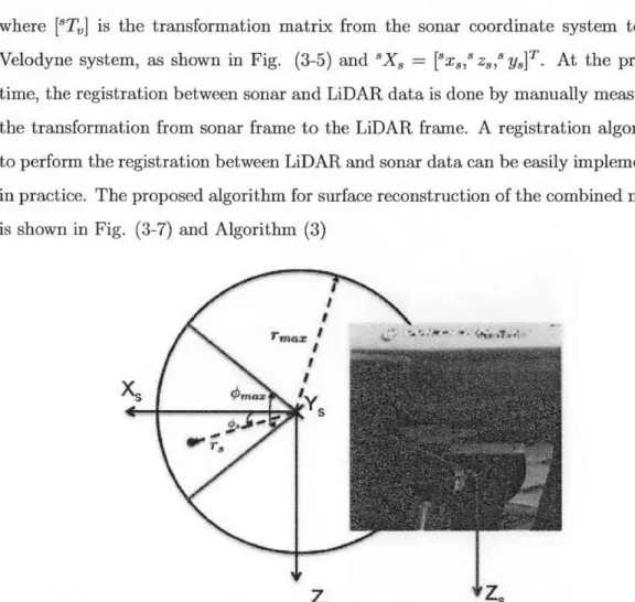
translation vector and the rotation matrix that transform the sonar data to the Velodyne coordinate system . . . . 57 3-6 Sonar coordinate system: Sonar gives returns up to a range of 10 m

with an angle of 45 degrees. . . . . 58 3-7 Surface reconstruction of both parts of marine structures, above and

below waterline. The ICP algorithm is used to find the transforma-tion matrices between different poses (using the laser scanner data). Then we use the transformation matrices to register the laser scanner data under the same coordinate frame and register the unregistered

2D sonar data as 3D data to the same coordinate frame. Then we use

a probabilistic framework such as the occupancy grid based maps to clean up the point clouds, and then we use known surface reconstruc-tion algorithms (ball pivoting algorithm and the Poisson reconstrucreconstruc-tion algorithm) to reconstruct a 3D surface model of the marine structure. 59 3-8 Filtering the sonar data. . . . . 61

(13)

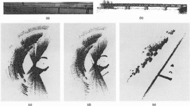
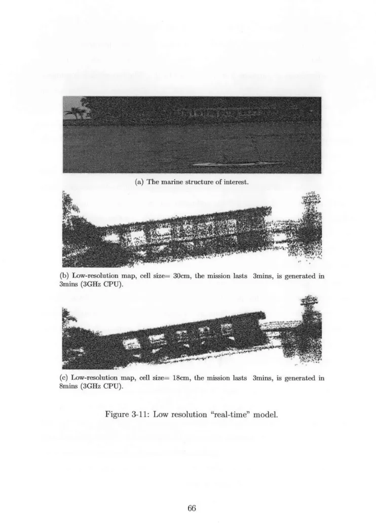
3-9 Reconstruction of a jetty in Pandan Reservoir, Singapore. (a) The

target jetty. (b) Side view of the jetty model constructed by our algo-rithm. (c) Top view of multiple frames of the 3D LiDAR data before processing. (d) Top view of the constructed 3D model based on GPS and compass information. (e) Top view of the constructed 3D model generated by our algorithm. . . . . 63 3-10 Reconstruction of a slowly moving boat in rough sea water

environ-ment, in Selat Pauh, Singapore. (a) Our operating area. (b) The target boat. (c) Side view of multiple frames of the 3D LiDAR data before processing. (d) Side view of the constructed 3D model based on

GPS and compass information. (e) Side view of the constructed 3D

model generated by our method. (f) Top view of multiple frames of the 3D LiDAR data before processing. (g) Top view of the constructed

3D model based on GPS and compass information. (h) Top view of

the constructed 3D model generated by our method . . . . 64

3-11 Low resolution "real-time" model. . . . . 66

3-12 The mesh-based high quality map for the above-water part of the jetty,

using a high probability threshold for occupied cells and the ball piv-oting surface reconstruction algorithm. Cell-size=8cm. . . . . 67 3-13 The mesh-based high quality map for the above-water part of the jetty,

using a low probability threshold for occupied cells and the ball pivoting surface reconstruction algorithm. Cell-size=8cm. . . . . 67

3-14 The mesh-based high quality map for the above-water part of the jetty, using a low probability threshold for occupied cells and the Poisson surface reconstruction algorithm. Cell-size=8cm. . . . . 68

(14)

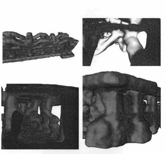
3-15 Zoom in of the mesh-based high quality map for the above-water part

of the jetty, using a low probability threshold for occupied cells and the Poisson reconstruction algorithm. Upper part, shows the pillars of the structure. Below left part, shows a surface of a human body (during the experiments we have people sitting and possibly moving on the jetty). Below right, shows two large buoys that are used to avoid direct collision of boats on the jetty. Cell-size=8cm. . . . . 69 3-16 Combined map: a) Picture of the front part of the structure. b) Point

cloud-based map, front view. c) Point cloud-based map, side view. d) Above- and below-water mesh-based map. . . . . 70 3-17 Upper part: A point cloud representation of the above- and

below-water parts of the structure. The color indicates the density of the points. Lower part: An occupancy grid based map of the above- and below-water parts of the structure. The color represents the probability of the cells to be occupied. Low probability gives blue colors and high probability gives red colors. . . . . 73 3-18 Comparison between our results and pictures of the actual jetty taken

from google maps. . . . . 73 3-19 Different types of oil platforms, the majority of the platforms are

float-ing and slowly movfloat-ing. The picture is from the Office of Ocean Explo-ration and Research . . . . . . . . 75

4-1 We can see the optimal control input (I*(t)), a representation of the optimal control input (u*(t)) and a control input that is close to the representation of the optimal control input (u(t) e.g. a control an algorithm that samples the control space returns). . . . . 84 4-2 Pendulum on a cart . . . . 98

(15)

4-4 Cart and pole simulation results. Upper: Simple-uniform without pruning. Middle: Simple-uniform with pruning. Bottom: ExpandTreeRRT with pruning. The iterations shown are the valid iterations (do not count collisions), the actual iterations are approximate 2 times more. 101

4-5 Pendulum on a cart, statistics (results obtained by choosing a node to expand uniformly and using pruning). Left hand side: the statistics for the case constant integration time At = is is used. Right hand side: the case the integration time is uniformly sampled from [0, 3s] is used. The iterations shown are the valid iterations (do not count collisions), the actual iterations are approximate 2 times more. . . . . 102 4-6 Close-to-optimal path as a function of time. . . . . 103

4-7 Close-to-optimal trajectory, in this case the integration time is uni-formly sampled from [0, 3]sec. . . . . 104 4-8 Holonomic agent in a space without obstacles: We can see the optimal

tree and the optimal trajectory at certain numbers of iterations. The

green area in the upper left part of each figure indicates the goal region. 105

4-9 Holonomic agent in a space without obstacles: the statistics for 50 runs

in logarithmic scale . . . . 106

4-10 The second case: two trajectories the algorithm returns for certain number of iterations and the statistics. . . . . 106

4-11 The second case: the statistics. . . . . 107

4-12 Dubin's airplane: Different views of a close-to-optimal trajectory (pre-liminary results). . . . . 108

5-1 For the biased-RITA, each node to be expanded is chosen with proba-bility proportional to the inverse of the density of the nodes within its neighborhood, here the first 3 nodes would be sampled with probability

2/8 and the last 2 with probability 1/8. . . . . 115 5-2 A cartoon illustration of v-partitioning. . . . . 119

(16)

5-3 First case study: we can see the average cost as a function of the

running time in linear scale (left part) and in log-log scale (right part). In the upper part of the figure we can see results generated using

Weighted-RITA, and in the lower part of the figure we can see results

generated using Uniform-RITA. . . . . 123

5-4 First case study, one run: The algorithm finds the first admissible trajectory (cost 120.6 units) after 0.7 seconds. The first admissible solution found does not belong to the same homotopy class as the op-timal trajectory. We keep running the algorithm, and at 71.5 seconds it switches to a different homotopy class and finds another admissible trajectory with cost 114.9 units. The algorithm improves the current solution within the same homotopy class (at time 117.3 seconds and cost 100.85 units). At time 171.4 seconds it finds another admissible trajectory with cost 92.5 units. After 400.3 seconds, it finds a bet-ter trajectory (this particular one of cost 68.7 units), which belongs to the same homotopy class as the optimal trajectory, and eventually this trajectory converges to a near-optimal one (63.8 units after 951.1

seconds). . . . . 124

5-5 First case study: Above part) Comparison between the trajectory that

the algorithm converges to and the optimal holonomic trajectory. We see that the optimal holonomic trajectory is close to the one the algo-rithm generates. Upper right and below part) The effect of additional obstacles (gray color) close to the structure of interest. . . . ..126

5-6 First case study: we can see the average cost as a function of the

running time in linear scale (left part) and in log-log scale (right part). In the upper part of the figure we can see results generated using Weighted-RITA, and in the lower part of the figure we can see results generated using Uniform-RITA. . . . . 127

(17)

5-7 Second case study, (a-d) the algorithm finds the first admissible

so-lution after running for 43.5 seconds (cost 219 units). It improves the current solution within the same homotopy class (113.7 seconds for cost 200 units). Then the algorithm explores few other homotopy classes and finally it converges to a trajectory with cost close to the optimal one (177.6 units in 51 min). (e-f) Different homotopy classes of trajectories with cost close to the optimal one. (i-j) Results with additional obstacles (obstacles in gray color). . . . 129

5-8 TSP-art-gallery approach: upper left shows the best inspection

tra-jectory out of 40 runs (cost 212 units), upper right: shows a typical trajectory (cost 265 units), lower right: the TSP solver failed to com-pute a good visiting order because the obstacles were not considered for the TSP problem, lower right: It fails to find a feasible trajectory because one of the observation points was chosen to be close to the obstacles. . . . 131

5-9 The size of marine structures and their mooring lines is huge. . . . 133 5-10 Top and isometric views of typical runs for each one of the missions.

a-b) optimal trajectory for the "ring" mission, c-d) close-to-optimal trajectory for the "knot" mission and in e-f) close-to-close-to-optimal trajectory for the "maze" mission. . . . 135 5-11 Several views of typical runs for each one of the missions. a-b)

close-to-optimal trajectory for the "oil rig" mission, c) a 3D CAD model of a real oil rig, d-f) close-to-optimal trajectory for the "Submarine" mission. 136

6-1 Effect of additive control and state noise . . . 146 7-1 The set of all path planning problems is a subset of the set of all

inspection planning problems and the set of all the inspection planning

(18)

(19)

List of Tables

5.1 Weighted-RITA: Average running times and iterations to get the first

feasible inspection trajectory and close-to-optimal inspection trajectories134

5.2 Uniform-RITA: Average running times and iterations to get the first

feasible inspection trajectory and close-to-optimal inspection trajecto-ries . .

(20)

(21)

Chapter 1 Introduction

1.1 Motivation

Autonomous inspection of structures is a complex problem with several applications to the marine, terrestrial and space environments. Efficient methods for structural

inspection have become increasingly important to ensure the safety and functionality of structures. Higher shipping traffic and increased terrorist threats demand faster and more frequent ship and harbor inspection. Likewise, greater demands on land

infrastructure create the need for faster bridge and road network inspection. The need for faster and more frequent structural inspection has increased the demand for structural inspection using autonomous robots.

Two essential parts of the autonomous (robotic) inspection problem are path

planning and surface reconstruction. The inspection (path) planning is the problem of finding an inspection trajectory that is informative enough to gather data (such as sonar and LiDAR data) from different views of a given structure that guarantee that all surfaces of the structures would be visible at a later time -during the algorithm execution. Given data gathered from all different views of a given structure, the surface reconstruction problem is the problem of registering all data under the same coordinate system to get a point based representation of the structure and then use meshing algorithms to reconstruct a 3D CAD model of the structure of interest. In this thesis, we focus on both the inspection planning problem and the surface

(22)

reconstruction problem. Another essential part of the autonomous inspection problem is the inference problem. In this part of the problem, the method performs inference over the obtained model to identify features of interest; in this work we do not focus on the inference part of the problem. Contributions (e.g. algorithms and theoretical results) developed in this thesis can be applied for any kind of structure such as terrestrial structures, road networks, bridges, space stations and marine structures. However, this thesis is motivated by the inspection of marine structures, and therefore

this is the focus of this work.

The inspection problem of marine structures is a very important problem with several applications including, evaluation and re-evaluation of the structures' condi-tion, identification of missing or broken parts, detection of foreign objects attached to the structures (e.g. mines or explosives), and navigation purposes. Depending on the application, the required resolution can vary from about 7cm (e.g. mine detection tasks) to 0.5m (missing or broken parts) or even to 1m for navigation tasks.

Marine structures are exposed to challenging conditions such as water currents, water waves, corrosion, and frequently several hurricanes per year. This exposure results in unpredictable damages to the marine structure, which could be life threat-ening for the people on and around such structures. Therefore, to ensure safety, thorough structural inspections are required regularly or after a platform is affected

by natural disasters. For example, after Hurricane Dennis in 2005 [15], structural inspection of Thunder Horse oil platform (Fig. (1-1)) was needed as soon as possible to identify damages on the platform and re-evaluate the platform's condition.

Currently, such inspections are performed by human workers through visual ob-servation. They inspect the above-water part of the structures aboard small boats, and use diving equipment for the submerged portions of structures. In Figure (1-2), we can see a diver inspecting the underwater part of a platform in the Gulf of Mex-ico [1]. In both situations, inspectors often lack the time and comfort to inspect the structures and re-evaluate structures' status properly. In addition, visual examination does not give inspectors the ability to track important structural changes. Scanning the structures, using robots, and automatically reconstructing 3D models from the

(23)

Figure 1-1: Thunder Horse oil platform after the Hurricane Dennis in 2005 [15]. scanned data would give the inspectors the opportunity to inspect structures from their offices, thereby reducing the safety risks of the inspectors and increasing the accuracy of the inspection results.

1.2 Challenges in the Inspection Planning

Prob-lem

Efficient methods for structural inspection have become increasingly important to ensure safety. Higher shipping traffic and increased terrorist threats demand faster and more frequent ship and harbor inspection. Likewise, greater demands on land infrastructure create the need for faster bridge and road network inspection. The need for faster and more frequent structural inspection has increased the demand for structural inspection using autonomous robots.

An efficient inspection planning algorithm is critical for developing such autonomous robots. Inspection planning is the problem of finding an inspection trajectory, i.e.,

(24)

Figure 1-2: Diver inspecting a platform in the Gulf of Mexico; the picture is taken from "TheOceanCorporation" [1].

a trajectory for the robot to scan all points on the structures. In this thesis, we focus on the inspection planning problem where the model of the structure and the environment are perfectly known prior to planning, and the robot has no control nor sensing error. More specifically, we would like to compute optimal or close to optimal inspection trajectories for robots with non-linear dynamics.

Although many inspection planning methods have been proposed, most are not suitable for robots with differential constraints. Most methods [29, 36, 37, 38] separate the inspection planning problem into two NP-hard problems and then solve each sub-problem sequentially. The first sub-sub-problem is the art gallery sub-problem, which finds the smallest set of observation points that the robot needs to visit to guarantee

100% coverage. The second sub-problem is the traveling salesman problem (TSP),

which finds the shortest trajectory to visit all observation points that have been generated by the art gallery solver. This separation approach is difficult to apply when the robot is non-holonomic and operates in cluttered environments, as the observation points generated by the art gallery problem may not be reachable from other observation points in the set. Furthermore, even if we generate the smallest set of observation points and even if we find the shortest trajectory to visit all points in the set of observation points, the generated inspection trajectory may not be the shortest trajectory for scanning all points on the boundary of the structure. In addition,

(25)

because most of the existing TSP solvers do not take into account neither vehicle dynamics, nor obstacles in the configuration space (e.g. the cost for connecting each one of the nodes is based on the euclidian distance), then the resulting visiting order results in trajectories that are far from optimal. In Fig. (1-3) we can see an example where the observation points are chosen correctly however the resulting trajectory is not close to optimal because the TSP algorithm computes the visiting order ignoring the obstacles. There is ongoing work on the multi-goal path planning community that tries to address the TSP problem in the presence of obstacles using heuristics (e.g. [114]), and in the presence of differential constraints without obstacles (e.g. [115]). Algorithms, presented later in this thesis can be used to address (in a probabilistic way, using randomized algorithms) the TSP problem in the presence of differential constrains and obstacles, however, this is not within the scope of our work. In short, most existing inspection planning methods are often not suitable to find a short inspection trajectory for robots with non-holonomic constraints.

9I

Figure 1-3: An illustration of a TSP-art-gallery approach: In this example, even if the observation points are chosen correctly the resulting trajectory is not close to optimal because the TSP algorithm computes the visiting order ignoring the obstacles.

In summary, because the computation of the observation points and the visiting order cannot be computed independently, even for holonomic systems, by separating the inspection planning problem to the TSP and the art-gallery problem optimal or close to optimal inspection planning may be impossible to be achieved. Instead, we model the problem as an optimization planning problem and we propose a solution based on tools and ideas developed by the path planning community and novel ideas

(26)

we present in this thesis. As we show later in this thesis this approach achieves optimal inspection planning.

A general way to define a planning problem is as follows. Given a dynamical

system, the obstacle free space (e.g. a subset of the state space that is obstacle free) and task specifications, we define an admissible path to be any obstacle free path that represents a solution to the system dynamics and does not violate the task specifications. Then an optimal task planning problem computes among all admissible paths the one that minimizes a cost function. The simplest category of task planning problems is the path planning problem; for the simple path planning problem an admissible path is an obstacle free path that starts from a given state, reaches the goal region and represents a solution to the system dynamics. Similarly, among all admissible paths the optimal path planning problem computes the one that minimizes a given cost function. In addition, for the optimal inspection planning problem we define an admissible path to be an obstacle free path that observes all details on a given structure. Figure (1-4) gives an overview of the path planning problem, the optimal path planning problem, the optimal inspection planning problem and the general task planning problem (for more details refer to the next chapters).

It is important to notice that it is extremely difficult to study the above problems in the state space since each planning problem (e.g. path planing, inspection planning, task planning) needs a separate analysis. In fact, the path planning community treats the inspection planning problem and the path planning problem in a different way separating it into the TSP and the art-gallery problems. Instead, of searching for an admissible path, if we search the control space for an admissible trajectory (path in the control space) similar analysis holds for each one of the planning problems. For instance, we assume that there is an optimal trajectory (control input) and our focus is to compute it (or approximate it). In this work, we will first study the simple path planning problem and then we extend our approach to the inspection planning problem.

Unfortunately, even the simple path planning problem is proven to be a PSPACE-hard problem, in fact it was proven to be a PSPACE-complete problem (with

(27)

re-Figure 1-4: Different planning problems: the path planning problem, the optimal path planning problem, the optimal inspection planning problem and the optimal task planning problem.

spect to the number of dimensions) [111, 117, 18]. PSPACE-complete problems are the hardest problems among all PSPACE problems, and PSPACE problems may be harder than NP problems (see Figure (1-5)). Because the dimensionality of the inspec-tion problem for agents with differential constraints can be large, this thesis introduces the use of sampling-based motion planners [21] to compute close-to-optimal inspection trajectories. Significant scientific work has been dedicated on sampling-based motion planners: Probabilistic RoadMap (PRM) [69], Expansion Space Tree algorithm (EST)

[61], Rapidly-exproring Random Trees algorithm (RRT) [80]; however, until today the

problem of asymptotically optimal motion planning for sampling-based motion plan-ners still remains an open problem for systems with differential constraints.

Sampling-based approaches [21], [81], are the most successful approaches for solv-ing simple path plannsolv-ing problems for high-dimensional systems. Up to a few years ago, sampling-based motion planners were only known to be probabilistically

com-Path Planning Optimal Path Planning Optimal Inspection Planning Optimal Task Planning

Given: Given: Given: Given:

[11 Dynamical system: [1] Dynamical system: [1] Dynamical system: [1] Dynamical system:

' (t) = f 0(t), U(t), t) ;Y(t) = f(-IM, u(t), t) X0t = 0~(t), u(t), 0) Wt = f(-Y(t), u(t), 0) [21 Free space: Si, [2 Pree space: St [2} ree space: Se. [21 ree space: Sje

[31 Initial state: Sin [3} Initial state: Sin [3J Initial state: Sin [31 Initial state: Sin

[41 Goal region: [4] Goal region: 141 Structure Primitives: [41 'ask specifications:

GoalfRegion c Stra GoalRegion C Sfee STR TASK

Compute: Define admissible path: Define admissible path: Define admissible path: [1] Path y : [0, Tc --+ S -y : [0, TJ - S such that Y : [0, TGJ -+ S such that y : [0, Tel - S such that

Such that:

Y(O) = Sin y(O) = Sin 'Y(0) = Sin ()= Sin

7(TG) E GoalRegion -y(Tc) E GoalRegion -y(t) E Str.Vt E [0,TGI 7(t) E Sfr.Vt E [0,Tcl

7(t) E SfreeVt E [0, Tc -(t) E Sfre.Vt E 10, Tca

Compute: UtCJ0TorG V(-y(t)) = STR, -y verifies all TASK

speci-where V(-y(t)) C STR fications

y* = argmaxmEr(D(y)), Compute: Compute: where:

D(y): Cost function *- = argmax_,Er(D(7)), y* = arg max1tr(D(-y)), r: Set of admiss. paths where: where:

D(₇): Cost function D(y): Cost function F: Set of admiss. paths F: Set of admiss. paths

(28)

PSPACE -^, NPC-LOG S ace O% Time%

Figure 1-5: The simple planning problem is a PSPACE-hard and a PSPACE-complete

problem (adapted from

[100J).

plete, in the sense that given enough time, they will find an admissible trajectory with probability one whenever such a trajectory exists. The question of optimality was addressed recently in

[671.

They developed sampling-based algorithms that are asymptotically optimal, such as PRM* and RRT*.l

Although PRM* and RRT* perform well for robots with simple dynamics, such as holonomic robots, extending asymptotically optimal sampling-based planners to systems with complex dynamics remains an open problem. The difficulty lies in the fact that both RRT* and PRM* perform their sampling in the configuration space and therefore require a steering function that drives the robot from one configuration to the other. Unfortunately, steering functions are often difficult to find and may not even exist for systems with complex dynamics, such as systems with non-holonomic constraints. We believe that for the general case, where we have non-linear under-actuated robots, sampling the control space directly may be a better choice. By sampling the control space directly, the difficulty of dealing with challenging dynamics and the necessity of the use of a steering function is alleviated. In fact, in this thesis we show that asymptotic optimality in sampling-based motion planning, inspection planning and general task planning (given the optimal admissible trajectory is a finite

1_{where asymptotically optimal means, given enough time, the probability the planner returns a} trajectory close to the optimal trajectory, is one.

(29)

time trajectory) can be achieved without the use of a steering function. Our analysis only requires Lipschitz continuity of the differential constraints and the cost function.

1.3 Optimality Through the Control Space

Currently, the optimality property for sampling-based motion planning algorithms that sample the state-space (e.g. RRT* [67]) is established only for linear-fully-controllable systems and a small subset of non-linear systems. The extension of the optimality proof for algorithms that sample directly the control space (without a steering function) is not obvious and it has been an open problem in robotics since

1997.

One of the key differences is that in the case we have a steering function and we sample points uniformly at random from the state space, e.g. the RRT* algorithm, each iteration of the RRT* algorithm is independent of the previous one. As a result the Borel-Cantelli lemma [67] can be used to show that the probability of sampling arbitrarily close to the optimal path approaches to 1 as the number of iterations increases. In the case the control space is sampled uniformly at random the above does not hold, and as a result Borel-Cantelli lemma cannot be used. In addition, the metric space used for the RRT* case (for fully controllable systems) is based on the Euclidean distance in the state space. In contrast, the approach we present in this thesis is general enough to use any cost function that is continuous.

1.4 Challenges in Surface Reconstruction by

Ma-rine Vehicles

There is a plethora of scientific work [95, 92] dedicated to the reconstruction of 3D models for land-based structures, however very few works have been dedicated to marine environments. Unpredictable disturbances such as water currents, and the marine environment itself pose significantly more challenges compared to the chal-lenges posed by terrestrial (shore) environments. Water currents generate disturbance

(30)

forces on marine vehicles, resulting in large roll and pitch angles. Furthermore, many marine structures are floating platforms, which move under strong currents. On top of that, GPS (Global Positioning System) access close to big marine structures is not reliable and other localization sensors developed for marine vehicles lag behind the ones developed for ground robots.

The 3D surface reconstruction problem often requires gathering 3D point clouds and registering them under the same coordinate frame. In the case of stationary structures, 2D laser scanners and localization sensors (GPS, Inertial Measurement Unit (IMU), Doppler Velocity Logger (DVL) or wheel encoders) can be used to gather

3D data from stationary environments [57]. In addition, advanced SLAM techniques

can be used to optimize the estimated trajectory and the resulting map [131, 116]. On the other hand, in the case of slowly moving structures special care should be taken in both gathering the 3D point clouds and registering them under the same coordinate frame. In the absence of knowledge over the motion of the structure, data gathered using 2D laser scanners combined with localization units cannot be used to reconstruct point cloud representations of structure views.

From our discussion above, it is clear that when dealing with moving structures,

3D laser scanners with a wide field of view that allows significant overlap between

subsequent laser scans should be used to gather point clouds. Then, registration al-gorithms that are invariant to motion, such as the Iterative Closest Point (ICP) [14], can be used to register all data gathered under the same coordinate frame resulting in a point cloud representation of the structure of interest. In the case of station-ary structures, researchers commonly use estimates of vehicle positions to initialize the ICP algorithm, [95], however this is not always feasible in the case of moving structures.

Part of this thesis (Chapter (3)) presents the hardware and software designs for scanning and reconstructing 3D surface models of marine structures. We alleviate the difficulty caused by disturbances, moving structures, and sensor errors by hardware and software design. In terms of hardware, we select sensors that would ease con-struction of 3D models from scanned data when no positioning sensors are available.

(31)

Furthermore, we develop a software system that constructs 3D point cloud models of marine structures from the scanned data and by using known surface reconstruction techniques reconstructs 3D surface models of marine structures. We have successfully tested our system in various conditions in Singapore waters between 2009 and 2011, including operating in the water with up to 2m/s water currents, and constructing

3D models of slowly moving structures. All the structures are constructed without

any information from positioning sensors, such as GPS and DVL.

The problem of reconstructing surfaces from registered point clouds still remains an open problem. There are several algorithms that reconstruct surfaces from point clouds, some of them reconstruct exact surfaces (interpolating surface) by a triangula-tion that uses a subset of the input point cloud as vertices [13], [5]. These approaches perform well in clean point clouds and present problems when the point clouds are noisy. Some other approaches reconstruct approximating surfaces by using best-fit techniques [55] [70], [3]. These approaches are robust to noise in the point clouds, however they tend to over-smooth the surfaces and thus important part of the struc-ture geometry may be lost. A comparison between several state-of-the-art surface reconstruction techniques can be found at [12].

1.5 Publications

Our surface reconstruction work was presented to several referee conference papers e.g. [76, 108] and published to Journal of Field Robotics (JFR) [107]. Our inspection planning work was presented to IEEE ICRA 2013 [102] and submitted to TRO [104]. Our path planning work is currently under-review to International Journal of Robotics Research [105], preliminary results can be found online in the "arXiv.org" [101].

An important part of robotics and especially marine robotics is the localization problem. It is well-known that there is no GPS access available underwater, this makes navigation of underwater vehicles a challenging problem. This thesis does not focus on the localization problem, however we have worked on the localization problem in previous contributions including several referee conference papers [106, 42, 41], a book

(32)

chapter published by Springer-Verlag [43] , and an International Journal of Robotics

Research paper [44].

1.6 Outline of the Thesis

In Chapter (2) we describe related work on both the path planning part of the prob-lem and the surface reconstruction probprob-lem. Regarding the path planning probprob-lem we will start with early results that explore the complexity of the problem and then focus on sampling-based motion (path) planners. In addition, we will also describe previous work on the inspection planning problem that use greedy methods, heuristics, and art-gallery-based approaches. We start the main part of this thesis with Chapter (3) where we describe hardware and software designs for scanning and reconstructing 3D surface models of marine structures. The proposed system was tested extensively in Singapore's coastal waters and a rich set of experimental results is presented. Doing the surface reconstruction experiments in Chapter (3), we realized how difficult is to compute robot trajectories that guarantee 100% structure coverage. The above open question motivated us to focus on the inspection planning problem which is modeled as a path planning optimization problem. In Chapter (4) we focus on the simple path planning problem; we provide an analysis that indicates that asymptotically optimal path planning can be achieved using sampling in the control space and thus asymp-totically optimal path planning for non-linear systems can be achieved without the use of a steering function. We also provide simulation results. Taking advantage of the analysis presented in Chapter (4), in Chapter (5) we provide a novel inspection planner that achieves asymptotically optimal inspection planning using sampling in the control space. A rich set of simulation results is provided. The planner devel-oped in Chapter (5) does not take into account uncertainty and noise. However, in Chapter (6) we study the robustness of close-to-optimal trajectories in the presence of control and state noise. In Chapter (7) we summarize our work with conclusions,

contributions and future work. In the Appendix (A) and Appendix (B) we derive some probability equations that are useful for Chapter (4).

(33)

Chapter 2 Related Work

2.1 Inspection Planning Problem

Given a perfect model of a structure, sensor specifications, robot's dynamics, an envi-ronment map and an initial configuration of a robot, an inspection planning algorithm computes an inspection trajectory (or path) that observes the entire surface of the structure of interest. The problem of inspection planning has attracted the interest of several researchers over the last 20 years. Choset's group proposed planners for cover-age, exploration and sensor-based coverage using cell decomposition methods [20, 22], Voronoi diagrams [2], and various heuristics [6]. Approaches based on cell decompo-sition methods yield good results but are restricted to low-dimensional state spaces. In this subsection we will concentrate on related work concerning inspection planning approaches (e.g. sensor-based coverage and structure coverage) whereas in the next subsection we will concentrate in the Coverage Planning Problem (CCP).

We first discuss early methods that discretize the free space, use graph represen-tations of the free space and search methods and heuristics to compute admissible paths. One of the first sensor-based coverage approaches for surfaces in 3D envi-ronments utilizes the use of 2D terrain-covering algorithms in successive horizontal planes laying at different depths and several heuristics. The proposed method can be used to map the seabed using AUVs (simulation results are provided) [51, 82]. The underling 2D terrain-covering algorithm uses cell decomposition methods and zig-zag

(34)

patterns to cover each one of the cells and their projected volume with respect the depth. Atkar et al. [8, 7] proposed the use of coverage algorithms for generating paths for autonomous/robotic painting applications. This approach utilizes a Morse decomposition method and a Reeb graph representation of the space that captures the topology of the surface of interest. It gives good results for the target application however it cannot handle additional obstacles in the configuration space and it is not scalable for different coverage problems.

Recently Cheng et al. [19] proposed a method that uses fine discretization op-timization methods to compute time-optimal trajectories that provide complete 3-dimensional coverage with applications to urban environments with 2.5-3-dimensional features. The basic approach is to approximate the features of interest with a set of non-planar coverage surfaces and to design a motion plan that guarantees the cov-erage surface is swept completely with a conical-field-of-view sensor. Simulation and experimental results are provided for a sensor attached to an unmanned aerial vehicle

(UAV).

Most of today's inspection planning methods can be divided into two approaches. One approach [29, 36, 37, 38] separates the problem into two sub-problems, the art-gallery problem and the TSP. Although most art-gallery solvers in computational geometry [99] do not consider sensor limitations, such as range limit, Gonzalez-Banos et.al. [48] have developed a method that takes into account sensor limitations. They use a randomized algorithm to select observation points that provide 100% coverage of the environment [47]. Danner and Kavraki [29] proposed the first randomized in-spection planning algorithm that uses a similar method to the one Gonzalez-Banos proposed to compute the guard points and then connects them to form inspection paths. The visiting order of the guard points is obtained by approximating the TSP solution; Danner and Kavraki also expand their work to simple 3D environments. A similar approach was taken by Englot and Hover [38] with application to complex

3D structures such as ship hulls. Their approach was probably the first one that

handles large structure sizes. Methods based on this separation approach often have difficulties to plan trajectories for robots with non-holonomic constraints operating

(35)

in cluttered environments, because some observation points generated by art-gallery solvers may be difficult or even impossible to reach from other observation points. Furthermore, these methods do not provide optimality guarantees, even if each sub-problem is solved optimally. Englot and Hover [38] provide a probabilistic complete-ness analysis of the algorithm and propose a smoothing algorithm that shortens the inspection paths by taking advantage of the asymptotically optimal RRT* algorithm; without guarantee of global optimality.

Another approach (e.g., [53]) relies on a sub-modular objective function to guar-antee that greedy algorithms generate near-optimal solutions. However, when the objective is to minimize the length of the inspection trajectory, as in our case, the problem is not sub-modular, and a greedy method may have difficulties as described in Figure (2-1).

404

R

L

Figure 2-1: An illustration of greedy strategy that always chooses to move to a configuration within R radius from its current position, that can see the largest unseen structure. The environment contains two structures, i.e., the "U" shaped at the bottom and the line at the top. In this example, the greedy strategy may fluctuate

moving down and up, while the shortest trajectory would move to cover the structure on the top first, before going down.

(36)

2.2 Coverage Planning Problem

A very similar problem to the inspection planning problem (e.g. the structure cov-erage problem, the sensor-based structure covcov-erage problem) is the Covcov-erage Path

Planning (CCP) problem. For a given visibility sensor, environment map and robot dynamics, the Coverage Path Planning is the task of determining an obstacle-free path that covers all the parts of the obstacle free space. An admissible solution to the CPP problem could also represent an admissible solution to the inspection planning prob-lem, however the opposite does not hold. Most of the previous CCP approaches deal with 2D workspaces, holonomic robots and assume disk-shaped sensor foot-prints with diameter of the same size of the robot physical diameter.

Choset and his group have studied the CPP problem extensively [23]. Among the first approaches they proposed were approaches based on cell decomposition methods.

All the cell decomposition based methods require:

" Exact decomposition of the free space into cells.

" Computation of the adjacency graph.

" Search methods to compute a path that visits all of the cells at least once.

" Local planning strategies to cover each one of the cells (e.g. zig-zag motion

pattern or mowing the lawn pattern).

The trapezoidal decomposition is the simplest cell decomposition approach that guarantees a complete coverage of the space [79]. Because it decomposes the space into trapezoidal shaped cells, each cell can be covered by simple back-and-forth mo-tion [98]. On the other hand, because of the simplicity of the trapezoidal shaped cells, this approach generally results in a huge number of cells increasing the difficulty of the problem. To address this problem, Choset and Pignon proposed the boustrophe-don cell decomposition method that takes into account the shape of the obstacles in the space and generates convex and non-convex shaped cells [241. Both the trape-zoidal cell decomposition and the boustrophedon cell decomposition can only handle

(37)

planar polygonal spaces. To address this issue, Acar et at. proposed a cell decompo-sition approach based on critical points on Morse functions [2]. The Morse-based cell decomposition approach can handle arbitrarily shaped obstacles in the state space.

By choosing different Morse functions arbitrarily shaped cells can be obtained (e.g

circular, trapezoidal etc.).

Another family of CPP approaches is the grid-based method that discretizes the free space into uniform grid-cells. As opposed to cell decomposition methods that

result in complete coverage, grid based approaches result in resolution-complete

cov-erage. Gabriely and Riman [45] developed the Spiral-Spanning Tree Coverage

grid-based approach that discretizes the free space into uniform grid-cells and uses algo-rithms (from graph-theory) to compute a tree that "visits" all grids. Zelinsky et at.

[135] proposed another grid based coverage approach; the proposed approach uses a

wavefront algorithm and gradient following methods to compute a path that passes from all grid-cells. Additional related work for the CPP problem can be found in

[23, 46].

2.3 Path Planning

Given a dynamical system, the obstacle-free space (e.g. a subset of the state space that is obstacle-free) and task specifications, we define an admissible path to be any obstacle-free path that represents a solution to the system dynamics and does not violate the task specifications. Then an optimal task planning problem computes an admissible path that minimizes a cost function. The simplest category of task planning problems is the path planning problem; for the simple path planning problem an admissible path is an obstacle-free path that starts from a given state, reaches the

goal region and represents a solution to the system dynamics. Similarly, among all admissible paths the optimal path planning problem computes the one that minimizes a given cost function. In addition, for the optimal inspection planning problem we

define an admissible path to be an obstacle-free path that observes all details on a

(38)

Early scientific work on the path planning problem has illustrated that the simple

path planning problem is an intractable problem [111, 117, 181. Studying the

"pi-ano mover's" problem (a simple path planning problem) using differential geometry methods Reif [111] has shown that the simple "piano mover's" problem (and there-fore the simple path planning problem) is a PSPACE-hard problem. Few years later, Schwartz and Sharir [117] proposed the first complete algorithm that solves the "pi-ano mover's" problem with doubly exponential running time. Given that Reif [1111 has shown that the simple "piano mover's" problem is a PSPACE-hard problem, it was unknown for about ten years whether the problem is PSPACE-complete problem or much harder. In his Ph.D dissertation Canny [18] proposed an exponential-time and polynomial-space algorithm illustrating that the path planning problem is in fact a PSPACE-complete problem.

Since the path planning problem is a PSPACE-complete problem, all practical algorithms that solve the path planning problem relax the completeness requirement one way or another. There are two families of practical path planning algorithms: the deterministic path planning algorithms and the sampling-based path planning algorithms. Deterministic algorithms often give up the completeness property, on the other hand, sampling-based planners relax the completeness requirement to the prob-abilistic completeness requirement. A sampling-based planner is called a probprob-abilistic complete algorithm if, given that an admissible trajectory exists, the probability will return an admissible trajectory approaches to one as the number of iterations increases

[21].

Much scientific work has been dedicated to the path/motion planning problems

[79, 21, 81]. Among the first path planning algorithms developed were the "bugi"

and "bug2" algorithms [89]. The bug algorithms use workspace information and very simple actions (e.g. the agent moves only on straight lines and follows the boundaries of the workspace). The introduction of the "configuration space" and the "free space" by Lozano-Perez [88] has enabled researches to study the problem in its correct base. Several approaches have been proposed including: potential fields

(39)

Planners based on potential fields construct a potential field on the configuration space in a such way that obstacles push away the agent and the goal configura-tion attracts the agent [71]. Thus an admissible trajectory can be computed using gradient-following methods. However, until today the construction of a potential field over a general configuration space that has a unique global minimum remains an open problem, thus these methods easily get trapped in local minima. On the other hand, discretization methods such as cell decomposition methods and decompositions based on Voronoi diagrams yield good results but are restricted to low-dimensional spaces. Over the past two decades, several sampling-based motion planners have been pro-posed. Sampling-based planners can be divided into two broad categories, i.e., graph-based approaches (multi-query) and tree-graph-based approaches (single-query). Graph-based approaches first construct a random graph in the configuration space and then use the graph to find admissible paths. This approach includes Probabilistic RoadMap (PRM)[69], [681, and it variants [125],[741,[35],[60], [4].

Tree-based approaches construct a random tree and stop construction whenever the constructed tree contains a path from a given initial configuration to the goal region. This approach includes the widely used Rapidly-exploring Random Trees algorithm (RRT) [801 and its variants e.g. [134]. Another type of tree-based sampling based planner is the Expansive Space Tree (EST)[61]. In terms of handling differential constraints, the main difference between the RRT planner and the EST planner is that the former performs its sampling in the configuration space and the latter performs its sampling in the control space.

Recently, Karaman and Frazzoli showed that RRT and PRM converge to a non-optimal trajectory and they developed asymptotical non-optimal planners e.g. RRT* and PRM* [67],[66]. However, a steering function is required to guarantee optimality and thus they are not suitable for general systems with differential constraints. Perez et al. [110] proposed the use of the RRT* algorithm combined with LQR methods to solve path planning problems with challenging dynamics. Similarly, Tedrake et al.

[126] proposed the LQR-Trees for feedback motion planning. However, these methods

(40)

of the RRT* do not hold for the LQR-RRT based algorithms. More recently, Dobson and Bekris

[331

proposed an algorithm that relaxes asymptotic optimality to near-optimality, to speed-up computing the solution. However, they still require a steering function.

One of the main contributions of this thesis is to perform an analysis on sampling-based motion planning algorithms and shed some light on its challenges. As we show in Chapter (4), asymptotically optimal planning can be achieved by directly sampling the control space. Furthermore, by modifying existing planners, we proposed a new family of asymptotically optimal planners. As the number of iterations increases, the control input these algorithms sample approaches the optimal control input.

2.4 Surface Reconstruction

The 3D model reconstruction problem can be considered a special category of the Si-multaneous Localization and Mapping (SLAM) problem [128]. SLAM was originally introduced by Smith et al. [123] and solved using EKF approaches and feature based maps [1241. Dissanayake et al. [321 prove that the solution to the SLAM problem is possible and propose another solution to the EKF-SLAM problem. Thrun, Monte-merlo et al. [129] [90] approach the problem from a probabilistic point of view, which was the foundation of the modern approaches that followed: Batch smoothing least squares optimization methods [31], its incremental equivalent [65] and incorporating loop closures [26] [27].

2.4.1 3D Model Reconstruction using Ground Robots

The 3D model reconstruction problem has attracted substantial research interest over the last 10 years. Although 3D model reconstruction by marine robots has not been studied extensively due to its difficulty, comparable processes have been researched using ground robots. Several robotic platforms were used and different mapping algorithms were proposed. Two different types of sensors (visual sensors and laser sensors) have been used, and each type has strengths and weaknesses.

Asymptotically optimal path planning and surface reconstruction for inspection