Automated inter-model parameter connection synthesis for simulation model integration

Automated Inter-model Parameter Connection Synthesis for

Simulation Model Integration

by

Thomas Ligon

B. S. Mechanical Engineering Rensselaer Polytechnic Institute, 2005

Submitted to the Department of Mechanical Engineering in Partial Fulfillment of the Requirements for the Degree of

Master of Science in Mechanical Engineering at the

Massachusetts Institute of Technology June 2007

C 2007 Massachusetts Institute of Technology All Rights Reserved

Signature of Author...

Department of g

May 29, 2007

Certified by... . .. ...

C>

Associate Professor of Mechanical Engineering Thesis Supervisor

A ccepted by ... . ... ...

Lallit Anand

MASSACHUSIrrS INSY himn

Automated Inter-model Parameter Connection Synthesis for

Simulation Model Integration

by

Thomas Ligon

Submitted to the Department of Mechanical Engineering on May 29, 2007 in Partial Fulfillment of the

Requirements for the Degree of Master of Science in Mechanical Engineering

Abstract

New simulation modeling environments have been developed such that multiple models can be integrated into a single model. This conglomeration of model data allows designers to better understand the physical phenomenon being modeled. Models are integrated together by creating connections between their interface parameters, referred to as parameter mapping, that are either shared by common models or flow from the output of one model to the input of a second model. However, the process of integrating simulation models together is time consuming, and this development time can outweigh the benefit of the increased understanding.

This thesis presents two algorithms that are designed to automatically generate and suggest these parameter mappings. The first algorithm attempts to identify previously built integration model templates that have a similar function. Model interfaces and integration models are represented by attributed graphs. Interface graph nodes represent interface parameters and arcs relate the input and output parameters, and integration models graph nodes represent interface graphs and arc represent parametric connections between interface graph nodes. A similarity based pattern matching algorithm initially compares interface graphs in two integration model graphs. If the interface graphs are found to match, the algorithm attempts to apply the template integration model's parameter mappings to the new integration model.

The second algorithm compares model interface parameters directly. The algorithm uses similarity measures developed for the pattern matching algorithm to compare model parameters. Parameter pairs that are found to be very similar are processed using a set of model integration rules and logic and those pairs that fit these criteria are mapped together.

These algorithms were both implemented in JAVA and integrated into the modeling environment DOME (Distributed Object-based Modeling Environment). A small set of simulation models were used to build both new and template integration models in DOME. Tests were conducted by recording the time required to build these

integration models manually and using the two proposed algorithms. Integration times were generally ten times faster but some inconsistencies and mapping errors did occur. In

general the results are very promising, but a wider variety of models should be used to test these two algorithms.

Acknowledgements

This thesis work would not have been possible with out the help of countless individuals. I will begin by thanking the mechanical engineering department for accepting me into their program and allowing me to learn at this great institute. I must also thank the Ford Motor Company. Employees at Ford first mentioned the possibility of an automated model integration function and planted the seed for this work to grow. And that seed would not have grown without the careful guidance of my advisor Professor David Wallace. Countless times he provided suggestions on how I could proceed or

things I should consider to help my work progress. I also used much of the work started

by Qing Cao and can not thank her enough.

I must also thank my fellow CADLAB students for providing either guidance, comic relief, or just a nice distraction to keep myself sane. In particular, I must thank Sittha Sukkasi, Sangmok Han, and lason Chatzakis for helping me learn DOME and all of its intricacies. I must also thank Alan Skaggs. He sat next to me in lab almost everyday for a year and a half amusing me with his stories, listening to my frustrations, and even giving me ideas when I was stuck.

Finally I must thank the countless people who made my time at MIT enjoyable. The wwednesday crew, whom I met during orientation, has been a great group of friends than are always fun to be around. I must of course thank my parents, even though they didn't completely believe I got into MIT when I first received the acceptance by

Table of Contents

1. Introduction 13

1.1 Context 13

1.2 Motivation and Problem Definition 13

1.3 Solution Overview 13 1.3.1 Introduction 14 1.3.2 Classification Method 14 1.3.3 Direct Method 15 2. Background 17 2.1 Search 17 2.2 Ontology 18 2.3 Pattern Matching 19 3. Classification Method 21

3.2 Pattern Matching Search Algorithm 21

3.2.1 Model Interface Representation 21

3.2.2 Graph-based Representation of Model Interfaces 22

3.2.2.1 Introduction to Graphs 22

3.2.2.2. Model Interface Fuzzy ARG 23

3.2.3 Graph Similarity Matching Algorithm 25

3.2.3.1 Introduction to Graph Matching 25

3.2.3.2 Similarity Measures 25

3.2.3.2.1 Attribute Similarity Functions 25

3.2.3.2.2. Node and Graph Similarity Functions 27

3.2.3.3 Graph Alignment Algorithm 28

3.3 Modifications to the Pattern Matching Approach 29

3.3.1 Introduction 29

3.3.2 Similarity Score Modification 29

3.2.3 Node Magnitude Difference Clustering Identification 31

3.4 Model Classification Output: Objective Match 33

3.5 Graph Matching Example 34

4. Integration Classification 39

4.1 Integration Models 39

4.1.1 iModels 39

4.1.2 Graph-based iModel Template Definition 39

4.2 Integration Classification Algorithm 40

4.2.1 Introduction 40

4.2.2 Algorithm Overview 41

4.2.3 Integration Algorithm Example 42

5. Direct Method 45

5.1 Introduction 45

5.3 Output-Input Mappings 46

5.4 Input-Input Mappings 47

5.5 Direct Method Example 48

6. Implementation and Testing 53

6.1 Implementation 53

6.1.1 Integrating Models in DOME 53

6.1.2 Classification Method Implementation 55

6.1.2.1 Implementation Overview 55

6.1.2.2 Algorithm Implementation Details 56

6.1.3 Direct Method Implementation 57

6.2 Testing 57

6.2.1 Introduction and Objectives 57

6.2.2 Models with Different Implementations 58

6.2.2.1 Goal 58

6.2.2.2 Model Interfaces 58

6.2.2.3 Results 61

6.2.3 Models of Different Magnitudes and Applications 62

6.2.3.1 Goal 62

6.2.3.2 Model Interfaces 62

6.2.3.3 Results 64

7. Conclusions and Future Work 69

7.1 Conclusions 69

7.2 Future Work 71

List of Figures

3-1 Simple Interface Causality Visualization 22

3-2 Model Interface Graph 24

3-3 Sample Bipartite Graph 28

3-4 Example Difference in Node Pair Magnitude Data 30

3-5 Beam Bending Situation Figures 34

3-6 3-Point Bending Graph 34

3-7 Cantilever Beam Point Load Graph 35

3-8 Bipartite Graph and Matching Results 36

3-9 Magnitude-Difference Plot 37

4-1 Integration Classification Algorithm Flowchart 42

4-2 Matched Bipartite Graphs 43

4-3 Integration Model Template 43

5-1 Causality Tracing Algorithm Flowchart 48

5-2 Electrical Heating Pipe Heat Transfer 48

5-3 Graph 1: Water Velocity Model 49

5-4 Graph 2: Constant Heat Flux Heat Transfer Model 49

5-5 Graph 3: Electrical Heating Element Model 49

5-6 Graphs with Final Mappings 52

6-1 Example DOME Integration Project 54

6-2 Example DOME Integration Model 54

6-3 Classification Results Frame 55

6-4 Mapping Results Frame 56

6-5 Single Turbine Interface 59

6-6 Impulse Turbine Interface 59

6-7 Multiple Turbine Interface 60

6-8 River Conditions Interface 60

6-9 Commercial Vapor-Compression Cycle Interface 62

6-10 Commercial Refrigerator Enclosure Interface 63

6-11 Residential Dual Vapor-Compression Cycle Interface 64

6-12 Residential Freezer-Refrigerator Interface 64

6-13 Ground Source Heat Pump Interface 65

6-14 House Heat Transfer Interface 65

6-15 Residential Refrigerator Mapping Results using the Commercial 67

List of Tables

3-1 Parameter Attributes 21

3-2 Initial k-Means Centers Data 32

3-3 Total Similarity Scores 35

3-4 Magnitude Similarity Scores 35

5-1 Similarity Scores Between Models 1 and 2 50

5-2 Similarity Scores Between Models 1 and 3 50

5-3 Similarity Scores Between Models 2 and 3 50

6-1 Multiple Implementation Integration Times 61

Chapter 1

Introduction

1.1 Context

Recently researchers have been developing modeling environment tools to enhance the design process. Examples of these design tools include MIT's DOME (Distributed Object-based Modeling Environment) [20,27], Phoenix Integration's ModelCenter [18], and Engineous' FIPER [8]. These modeling environments make use of internet based infrastructures to facilitate the distribution of simulation models, and parametrically combine multiple models into complex integrated models.

The vision of these tools is to provide an enabling technology for a World Wide Simulation Web (WWSW). This WWSW would allow engineers, scientists, and

designers to share their models and develop a simulation model community. This sharing of models accelerates the exploration of design tradeoffs, optimization, and model validation. The models existing on the WWSW could also be integrated into a single model, encompassing the work of numerous people and compiling the results from each model. The integration of multiple simulation models can greatly improve the global knowledge and understanding of the physical processes which are being modeled.

1.2 Motivation and Problem Definition

Generally teams of people work together to solve complex problems that require numerous simulation models. Results from these models may be interrelated and

information must pass between them, but the models themselves may be distributed around the world. Modeling environments such as DOME bridge the gap between these models and ideally allow the designers to view all of the models working together.

Integrating these models together, however, can be a time consuming process for large models. In DOME, the designer must prescribe how models map together. A mapping can be thought of as an equality relation between two parameters in two

different models. Once two parameters are mapped together, they act like a single parameter. Mappings can be created between common input parameters, or between an

output parameter from one model and an input parameter from a second model. This process of creating mapping relations between model parameters is how models are integrated in DOME.

Designers are commonly developing models with hundreds. if not thousands. of parameters and might wish to integrate numerous models. The creation of all the parameter mappings could take days if not weeks, time which should be spent using the models to analyze the problem and generate a solution. The intention of this thesis work is to develop an algorithm for automatically generating inter-model parameter relations to efficiently integrate simulation models.

1.3 Solution Overview

1.3.1 Introduction

The following chapters will detail two approaches for the generation of inter-model parameter relations to integrate simulation inter-models. This section will introduce two approaches to solve this problem. The first approach is called the classification method and the second approach the direct method.

1.3.2 Classification Method

This approach was developed in order to take advantage of a WWSW. Designers publishing models to servers available all around the world would provide a great wealth of simulation model integration knowledge. The integration models contained on these servers can serve as a guide for integrating different models for a similar purpose. For example, a large automotive company might have previously developed an integration model which represents the drive train for one of their trucks. Currently they are in the

process of developing models for a new car in their lineup. The models for each component in the car drive train might be different, but the parameters which must be mapped together in the models might be identical to the parameters which map together

in the truck drive train.

With the existence of a WWSW, model integration knowledge would be readily available. However, determining which integration model accurately represents the integration model the designer wishes to produce is a difficult task. This approach breaks the process down to three steps.

1. Search for similar models on the WWSW for each individual model the designer

wishes to integrate. These models will be referred to as objective models.

2. From this set of similar models, search for integration models which contain this set of similar models, and verify that the mappings in the integration models actually exist between the objective models.

3. Implement the mappings present in the WWSW integration model between the

objective models.

This approach attempts to "classify" the designer's objective models as similar to models found on the WWSW. Using these similar models it will attempt to "classify" the integration model based on integration models found on the WWSW. Therefore, this approach will be referred to as the classification method.

1.3.3 Direct Method

The second approach is meant to handle situations when the classification method is unsuccessful. This approach compares two objective models directly and uses a set of heuristics to find parameters which are extremely similar. This method is likely prone to error but with added input from the designer, should prove to be beneficial to the model integration process. This approach compares models directly and will be referred to as the direct method.

Chapter 2

Background

2.1 Search

The classification approach proposed in the previous chapter is fundamentally a search problem. Given a set of model interfaces, this approach must search for a similar set of model interfaces that have already been mapped together. The approach described previously requires a search for both model interfaces and integration models. The model

interface search problem has already been studied by Qing Cao [1]. Cao proposed a pattern matching approach which will be discussed in more detail in chapter 3.

Search problems are encountered in many fields and a pattern matching approach is not the only option. The most familiar search problem involves searching the World

Wide Web (WWW). The simulation model design environment envisioned in this work would appear very similar to a WWW, and considering WWW search techniques would

seem very appropriate.

Searching the web has been approached by using semantics, associating a meaning to information contained in web pages that a search algorithm can understand. This has been a prominent field for research, the most notable project being the Semantic Web project

[26]. A Semantic Web works by "marking up" web pages with semantics which can be

content based descriptions or tags. The languages for these "mark-ups" come in a number of forms including the customizable Extensible Markup Language (XML), the Resource Description Framework (RDF), and the Web Ontology Language (OWL).

The entire WWW is not entirely a Semantic Web. The World Wide Web Consortium (W3C) has been attempting to distribute semantic web standards in hopes of the entire WWW adopting them. It was recently reported that 1.3 million Semantic Web documents

were found on the WWW in March 2006 [9]. These Semantic Web documents aid search algorithms in "understanding" web pages that will enable searches based on concepts and not just keywords.

2.2

Ontology

Ontology's roots are in Philosophy. In philosophy, ontology attempts to define

existence by describing its basic categories and relationships. Ontology has now made the jump to computer science, and one of its formal definitions, "specification of a

conceptual classification" was presented by Gruber in 1993 [10]. More simply, an ontology is a universal description of a concept or rule.

An ontological approach for search would require semantic markups to be written as formal ontologies. Any data that needs to be searched must have these ontologies embedded. Because an ontology has a universal definition, search algorithms can easily interpret the data using rule-based inference.

This approach is very appealing when the searchable data falls into very specific categories that can be described by an ontology. However, model interfaces are not necessarily easily categorized. The landscape of modeling is constantly changing. The types of models, modeling programs, modeling capabilities, and even the means for representing the data can change. This continuously changing environment makes the development and enforcement of ontology use extremely difficult. New developments would require new ontologies that would need to be accepted by the modeling

community at large. This process would be time consuming, not including the time required to markup the simulation model interfaces with these ontologies [13].

The ontological approach is very exciting because by using it the inference of data is fast and very precise based on specific ontological definitions. Unfortunately, in this application the data environment is very heterogeneous and constantly changing making use of ontologies extremely difficult.

2.3 Pattern Matching

Pattern matching algorithms attempt to discover the existence of a given pattern in data. Generally these patterns have a given structure of multiple parts. The data structure can take many forms including trees, sequences, and mathematical graphs [31]. A very common pattern matching application is image retrieval where colors, shapes, and spatial locations are used to identify patterns [16]. Similarity matching algorithms can be used to classify image components based on their colors etc. The structure of these image

components can then be compared.

The advantage of pattern matching algorithms is that a fixed knowledge base is not required. The matching algorithms can handle a large variety of patterns and components. However, the explicit relationship between these patterns and the particular functions of the data is not known. Another problem can arise when patterns do not match exactly. Heuristics might be required to make the required distinction between patterns which match, or do not match. Pattern matching is most advantageous when correlation between the data structure and its functionality are apparent and a specific degree of matching is not required. Because this work envisions the final matching decision to be made by the user and the structure of models can be functionally significant, the pattern matching approach appears to be appropriate.

Chapter 3

Classification Method

3.2 Pattern Matching Search Algorithm

3.2.1 Model Interface Representation

Before the pattern matching algorithm developed by Cao can be introduced, it must be understood what model information is available, and how a recognizable pattern can be established. There has been some work in developing engineering design

representations [23,24], however, they generally require the full definition of the model. The World Wide Simulation Web (WWSW) envisioned in this work would not require the full model definition. Models which are functionally equivalent could have different implementations but yield identical results. This is the theory behind DOME models.

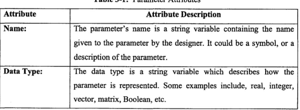
In DOME, all models are represented by a common interface definition. This interface contains a list of all the input and output parameters and the inter-parameter dependency or causality information, which input parameters each output parameter depends on. Each parameter has five attributes: name, data type, unit, magnitude, and whether it is an input or an output parameter.

Table 3-1: Parameter Attributes

Attribute Attribute Description

Name: The parameter's name is a string variable containing the name

given to the parameter by the designer. It could be a symbol, or a description of the parameter.

Data Type: The data type is a string variable which describes how the parameter is represented. Some examples include, real, integer, vector, matrix, Boolean, etc.

Unit: The unit is a string variable which contains the S.I. or English system unit. The parameter can also be dimensionless.

Magnitude: This is a double variable which contains the parameter's numerical magnitude.

Input/Output: The parameter can either be an input or an output. Parameters which are intermediate values are still considered outputs.

Figure 3-1 depicts DOME's visualization of a model interface. This extremely simple model calculates the cost of an item based on its length and width. The cost is dependent on the width and length variables which are shown visually using arrows. The model that

calculates the cost could be anything, for example a Microsoft Excel spreadsheet. 4 Width

S

9

Figure 3-1: Simple Interface Causality Visualization

3.2.2 Graph-based Representation of Model Interfaces

3.2.2.1 Introduction to Graphs

Graphs are mathematical tools that have been used to model many different types of data and data structures. Some applications include modeling molecules in chemistry and biology, networks (computer and traffic), and many areas in pattern recognition [30]. There have been many different graph representations developed over the years and the representation suggested by Cao is an attributed relational graph (ARG), first developed

by Tsai and Fu [25]. The graph is comprised of nodes that are connected by arcs. The nodes generally represent objects and the arcs describe the relations between the nodes.

Attributed relational graphs are generally separated into two classes. The first is based on probabilities and is known as a random graph. The first random ARG's were modified for pattern matching by Wong et.al. [32]. However, random graphs require large training sets and are not appropriate for simulation model interfaces which may only have several functionally similar instances.

The class chosen by Cao to represent model interfaces is based on fuzzy set theory, introduced by Dr. Lotfi Zadeh [33]. Fuzzy sets contain elements that are characterized by a membership function p. This function represents the degree of membership of each element to the set and generally ranges from zero to one. The first fuzzy ARG was used to represent Chinese characters and was developed by Chan and Cheung [2]. A Fuzzy ARG differs because its nodes and arcs are represented by fuzzy sets and have

membership functions. The nodes and arcs are no longer concrete. They have a degree of membership and missing data can be estimated using fuzzy methods [16].

3.2.2.2 Model Interface Fuzzy ARG

The fuzzy ARG for a simulation model interface developed by Cao represents

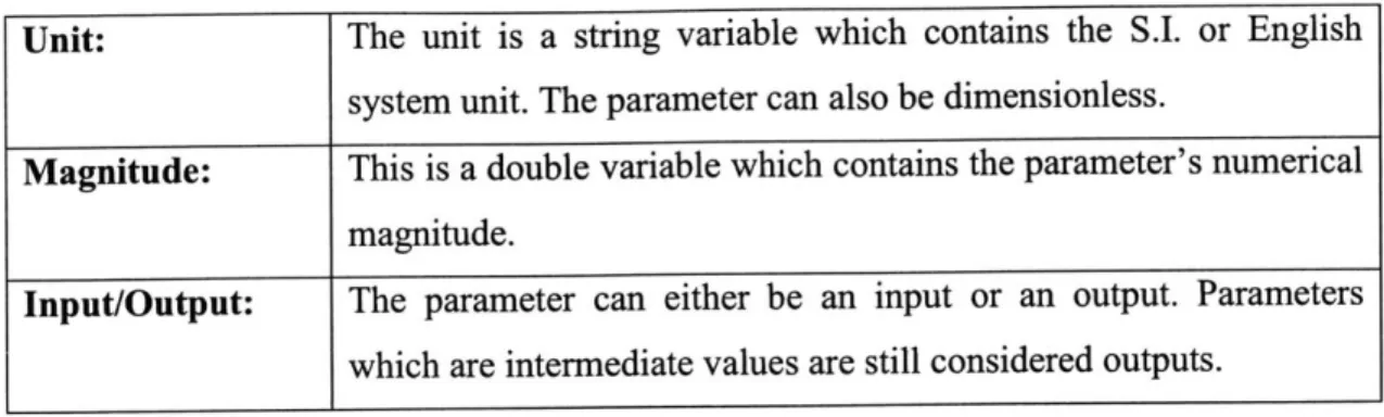
parameters as nodes, and arcs are connections between an input node and an output node. Nodes contain the five attributes presented as available in model interfaces, and the arc direction is such that input nodes drive output nodes. The ARG is fuzzy because each node attribute can be a set of attributes from multiple functionally similar model interfaces. Each node and arc is weighted, indicating the number of times a node or arc occurs when multiple model interfaces are combined into a single fuzzy ARG. The model interface fuzzy ARG is known as a template because it represents a functional model and is not necessarily a single model interface. The formal definitions for a template fuzzy ARG and its components are given in definition 3-1 through 3-4 (these definitions were taken directly from Qing Cao's PhD thesis [1]).

Definition 3-1: A fuzzy set variable (of node attribute) is defined as:

X = {xA ,x,.. ,J,. ,--,x/1 0, where xi indicates the ith state of the variable x and

#

indicates the number of times such state was asserted (number of occurrences).

Definition 3-2: A template node is defined as:

N =

{xn

J,

variable of the name attribute for that particular node, and so forth.

Definition 3-3: A template arc ai connects a template node Nj to the node Nk and it

is denoted by a, = (N,,N, ) , Arcs do not contain any attribute.

Definition 34: A template graph is defined as:

G" =INI ,N20 ,..Nf .. ,Nl am , a ,... avi ,.. Id, where Ni is a template node defined in Definition 4-3(a); ai is a template arc defined in Definition 4-3(b).

This template definition of a functional model is what would exist on a WWSW and be the basis that an objective model is classified. The objective model can also be represented by a fuzzy ARG, but all nodes and arcs would have a weight of one. Figure

3-2 depicts an example template graph for a model interface.

Name: Length Name: Width Name: Height

Data Type: Real Data Type: Real Data Type: Real

Unit: Meters Unit: Meters Unit: Meters

Magnitude: 2 Magnitude: 0.5 Magnitude: 10

In/Out: Input In/Out: Input In/Out: Input

Name: Volume Data Type: Real Unit: Cubic Meters Magnitude: 10 In/Out: Output

3.2.3 Graph Similarity Matching Algorithm

3.2.3.1 Introduction to Graph Matching

The Attributed Relation Graph (ARG) for simulation model interfaces previously presented provides a structure that facilitates the use of a pattern matching algorithm. Many graph matching algorithms primarily use the graph's topological structure as the basis for matching [reference]. In this case, however, the information embedded in the node attributes is essential in determining a model interface's functionality. Two models can be topologically identical, yet functionally dissimilar.

Similarity measures can provide a means for relating the node attribute data. The topological data in this case relates the interface causality information. If the similarity between node attributes is high, the topological data serves only as verification that the nodes are aligned in a similar fashion. This is the concept behind the pattern matching algorithm developed by Cao. Similarity measures were developed in an attempt to relate the functional similarity of two model interface graphs. These measures are presented in the following section.

3.2.3.2 Similarity Measures

The similarity measures developed by Cao all range in value from [0,1]. The score is evaluated in pieces starting with each node attribute, which are combined to calculate a node similarity score, and are finally used to calculate a graph similarity score.

3.2.3.2.1 Attribute Similarity Functions

A node has five attributes, and each attribute has a similarity function associated with

it. The name attribute is a string of words and characters. There are many different string similarity measures available and Cao chose measures developed by Jaro [12] and Winkler [28] which has been found to yield some of the best results [5]. The Jaro-Winkler algorithm was paired with a pubic domain algorithm library [4] to assign a similarity score for the name attribute.

Cao developed a similarity function for the data type attribute (real, integer, matrix, etc.). For example this function would relate real parameters to integer parameters. However, in this work the data type must match exactly for mapping to occur. Therefore, this function reduces to the binary function given in equation 5-1.

)(X 0

s xdatatype _{a 5 Xdatatype b =}

-different data type.

same data type. (Equation 5-1)

The input-output similarity function is also a binary function, shown as equation 5-2. Input parameters can not be matched to output parameters and vice versa.

1 if Xinouta = Xinoutb e inputs

s(xiouta,xiul,) b 1 I i xiu, a x X , br outputs (Equation 5-2)

10 otherwise

The unit attribute's similarity function has two steps. The first step must determine whether or not the unit's fundamental dimension is compatible. The unit's dimension, as defined in dimensional analysis [21], is a combination of the fundamental dimensions length [L], mass [M], time [t], etc. Units must be dimensionally identical, therefore, the similarity function reduces to a binary function where identical dimensions receive a similarity score of 1 and dissimilar dimensions a score of 0.

The second step involves scaling each unit to a base dimension scale. A real value for the unit is assigned based on the base scale [19]. For example, a unit of dimension length

is scaled to meters. If the dimension is in millimeters, a real value of 0.001 is assigned. The similarity function calculates a similarity score based the unit's assigned value

shown in equation 5-3.

s(xu,

A similarity function for the magnitude attribute was also developed. However,

the magnitude similarity function is very coarse. Initially, each magnitude value is scaled to its base power of 10. A value of 0.004 would be scaled to 0.001, and a value of 17 would be scaled to 10. A log based similarity score was then assessed. The goal of this work is to identify model interfaces which are extremely similar to enable accurate parameter mapping. Therefore, this similarity function was revised and the new function will be presented in a later section.

3.2.3.2.2 Node and Graph Similarity Functions

The similarity between two nodes is calculated as the average of the magnitude, name, and unit similarity scores. A score of 0 is assigned if any of the attribute similarity scores are 0.

Equation 5-4: Let an objective interface node be n = {Xname Xdim , XiXyeXi 1 ; let

a template node be N ={Xame 9 Xdim, X ,, Xdype X I,, ,,, the similarity score is calculated using equation 5-4.

s~x , .)+s~.,,X.,)+s~.,,,,,X , SXdy

s(x .eXn n,~,, ) + S(XXit=, Xuit)+ + mag ni , Xd)=1,smx , 1, 19 ,, , X ,x , 1;

s(n,N) =

0 otherwise.

(Equation 5-4)

The graph similarity score is calculated using nodes which have been aligned by the pattern matching algorithm, to be described in the next section. The similarity score attempts to describe the overall match of the two graphs. Let an objective interface graph

be g ={n,,n,,--,n; a,, a2,.--,ak} and a template graph be

G N, ,N0 ,N ,.,; a ,..., af ,...,a }. Because the similarity score is

calculated using aligned node pairs, let p be a node pair. Let n,, be a node in the pair from the objective interface graph g and Np be a node in the pair from the template graph G. Equation 5-5 calculates the similarity score between g and G.

Equation 5-5: Let bN, be the number of occurrences of node Np within G, where pi is the it

h pair of aligned node pairs.

#Pairs

E P , .N ,

s(g, G) - ,, (Equation 5-5)

ONi

3.2.3.3 Graph Alignment Algorithm

Graph alignment is performed using a maximal bipartite matching algorithm. A bipartite graph is another type of graph used in graph-theory. A bipartite graph is special because it contains two distinct sets of nodes where arcs do not connect nodes from the same set [29].

First Node Set

A 0C

D F

ZY X W

Second Node Set

Figure 3-3: Sample Bipartite Graph

In this application, the bipartite graph is formed using nodes from an objective graph as the first set, and the nodes from a template graph as the second set. Similarity

scores are calculated for every objective-template node combination. The initial bipartite graph contains arcs which represent all of the non-zero similarity scores between the nodes. It is important to understand that each node could be connected with multiple arcs.

The bipartite matching algorithm maximizes the graph similarity score while only allowing each objective interface graph node to be matched to a single template graph node.

After the bipartite matching algorithm has maximized the matched node pairs, the arcs from the fuzzy ARGs are introduced to verify the matching. Input matched node pairs must be identically connected with arcs to the output matched node pairs. An arc which connects a paired input node and a paired output node in the objective graph must also exist in the template graph connecting the objective graph input node and output nodes matches. If none of the arcs that connect a node in the objective correspond to the arcs in the template graph, the matched pair is rejected. If a matched node pairs was verified, its similarity score is used to calculate the final graph similarity score using equation 5-5.

3.3 Modifications to the Pattern Matching Approach

3.3.1 Introduction

The pattern matching approach described above generates a similarity score for each objective model-template combination. The score is based on similarity metrics for three of the five parameter attributes: name, unit, and magnitude. This similarity score is a relative metric and is generally meaningless.

The objective of this work was to quantitatively classify each model based on template model representations distributed on a WWSW. If the pattern matching approach previously described is to be used, the similarity score calculation must be modified in order to achieve accurate classifications.

3.3.2 Similarity Score Modification

The method for calculating the model-template similarity score must provide some quantitative metric which can be used to make the decision as to whether an objective model and a template are functionally similar or not. This score must still be based on the three parameter attribute similarity metrics. However, the parameter similarity score does not need to be modified because it is still appropriate for the bipartite matching phase of the pattern matching algorithm. Therefore, two sets of parameter similarity scores will be

calculated. The first parameter similarity score remains unchanged and is the average of the three similarity metrics.

The second parameter similarity score will include only the parameter magnitude similarity metric. However, the magnitude similarity score described by Cao is not appropriate. Instead, a new logarithmic-based equation, equation 5-6, is suggested.

Equation 5-6: Let x be the objective graph node magnitude and X be the template

graph node magnitude.

S(xnagntude , Xmagnitude b I -10. l(absilog₁0 (Xmagnitude log ₁₀ (Xa,,itude)l) (Equation 5-6)

This similarity equation again provides a score between 0-1, but now each tenth is a difference in the magnitude of the two nodes of a power of 10. A similarity score between 1-0.9 indicates the two nodes have magnitudes within one power of 10 of each

other. The objective-template graph similarity score can be calculated using this second parameter similarity score given in equation 5-7.

Equation 5-7: Let g be an objective interface graph and G be a template graph. #Pairs

Z

s#(g, G)= #P.(Equation 5-7)

This new objective-template graph similarity heuristic provides a quantitative functional similarity measure. If a graph similarity score of 0.9 is achieved, it is known that the average node pair magnitude difference is within one power of ten.

The value of 0.9 will be used as the cutoff for functional similarity for this work. However, this is actually a relatively strict metric. An extremely simple example of the failure of this metric is a simple volume calculation. Liquid volumes can range from milliliters to kiloliters, but the calculation for this volume of liquid in a cylindrical

required to handle this possibility because the similarity score would be below the 0.9 threshold and the graphs would not be considered a match.

3.3.3 Node Magnitude Difference Clustering Identification

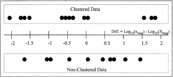
Models which are functionally similar may have vastly different magnitudes. A 0.8 liter 2 cylinder go-cart engine would certainly be functionally similar to an 8 liter 10 cylinder automobile engine, but many of their parameters could differ in magnitude by greater than one order of magnitude. However, it is possible (and is also the assertion of this thesis) that models which are functionally similar but of different magnitudes will contain parameters whose differences in magnitudes, if plotted, will form distinct clusters. Therefore, the identification of clustering in the difference in node magnitudes would be a sufficient condition for objective-template graph functional similarity. Figure 3-4 depicts this clustering.

Clustered Data

Diff. = Logl₀(xna ) -Log₁o(Xma)

-2 -1.5 -1 -0.5 0 0.5 1 1.5 2

0 - - 0-- --- 0 * 0

Non-Clustered Data

Figure 3-4: Example Difference in Node Pair Magnitude Data

A number of common clustering algorithms exist including a family of algorithms

known as Expectation Maximization (EM) algorithms. EM algorithms attempt to

maximize the probability a data point falls under a cluster distribution. EM was formally introduced by Dempster in 1977 [7]. K-Means is an example of an EM algorithm which was introduced by Cox [6] and refined by Hartigan [11]. K-Means uses a distance measure to calculate the distance between data points and a cluster center and assigns

each data point to a cluster center. The center is then recalculated and the process is repeated. The algorithm will iterate until the data points no longer jump between different cluster centers.

The advantage of expectation maximization algorithms, and especially the k-Means algorithm, is that they are generally very fast. However, k-Means requires the number of clusters to be known, and then it optimizes their position. There are algorithms which analyze the data to determine the numbers of clusters present including the v-fold cross-validation algorithm [3]. However, this is yet another step and there are heuristic based methods which can adequately solve this problem.

The clustering algorithm chosen was the k-Means algorithm because it is fast and easy to implement. The k-Means algorithm has three basic steps.

1. Distance Calculation between each cluster center and each data point.

2. Assignment of each data point to a cluster center

3. Recalculate the cluster center as the average of all of its member data

points.

Repeat until data points no longer jump between clusters.

The problem of not knowing the number of clusters will be handled by running the clustering algorithm multiple times and incrementing the number of clusters used

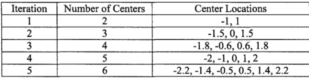
each time. Table 3-1 outlines how many centers, and their initial locations, are used during each of the iterations. The centers change after each iteration to ensure false clusters are not identified.

Table 3-2: Initial k-Means Centers Data

Iteration Number of Centers Center Locations

1 2 -1,1

2 3 -1.5,0,1.5

3 4 -1.8, -0.6, 0.6, 1.8

4 5 -2,-1,0,L,2

After each iteration the cluster centers are identified, and their standard deviations are added to an array of cluster centers. A cluster center is only added to the array if it has associated data points. Generally if the number of clusters assumed to exist is greater than the number of clusters which do exist, the remaining cluster centers will have zero data points associated with them. If a cluster center that is to be added already exists, the number of times which it was identified is stored. This process is repeated until five iterations have completed or until no new cluster centers are identified.

This cluster data must then be analyzed to determine if clustering truly exists. The simplest situation is when none of the cluster centers were ever repeated. If this occurs, clustering is assumed to not be present. For clustering to be present, a necessary and a sufficient condition are proposed. The necessary condition is that cluster centers must have been repeated and must contain the majority of data points greater than fifty percent.

The sufficient condition states that the cluster distributions are relatively tight and do not significantly overlap. The sufficient condition is very qualitative and in this case will be made quantitative using heuristics. The two metrics are a maximum allowable standard deviation and percent overlap in the distributions. The maximum allowable standard deviation is 0.3 and the distributions can not overlap out to two standard deviations. This is not a particularly appropriate solution, but is convenient in order to demonstrate the validity of the clustering approach.

3.4 Model Classification Output: Objective Match

If an objective model interface was classified by an interface template, the

classified objective-template pair is stored as an objective match. An objective match stores the objective model interface graph, the interface template graph, and an array containing each objective-template node pair. The final output from the model

classification algorithm is an array containing all of the objective matches which were found. The formal definition of an objective match is given below.

Definition 3-6: A node pair p, that pairs together an interface graph node n, and a

template graph node Np, is defined as p = (n, N,).

Definition 3-7: An objective match M, that pairs together an objective graph g with a template graph G, is defined as: M =

{g;G;pP

}

{pP

node pairs.

3.5

Graph Matching Example

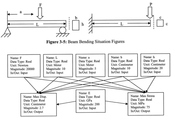
The following example will illustrate the classification method using two beam bending model interface graphs. The first model is a cantilever beam with an end point

load, and the second model is a beam undergoing 3-point bending. Figure 3-5 depicts the two beams to be modeled, and figures 3-6 and 3-7 depicts the graphs for these models.

F P

b c

L h L c

////

Figure 3-5: Beam Bending Situation Figures

Name: F Name: L Name: a Name: b Name: h

Data Type: Real Data Type: Real Data Type: Real Data Type: Real Data Type: Real

Unit: Newton Unit: Meter Unit: Meter Unit: Centimeter Unit: Centimeter

Magnitude: 20000 Magnitude: 10 Magnitude: 5 Magnitude: 10 Magnitude: 20

In/Out: Input In/Out: Input In/Out: Input In/Out: Input In/Out: Input

Name: E

Name: Max Disp. Data Type: Real Name: Max Stress

Data Type: Real Unit: GPa Data Type: Real

Unit: Centimeter Magnitude: 200 Unit: MPa

Magnitude: 2.7 In/Out: Input Magnitude: 75

In/Out: Output In/Out: Output

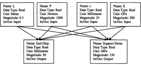
Name: L Name: P Name: c Name: E

Data Type: Real Data Type: Real Data Type: Real Data Type: Real

Unit: Meter Unit: Newton Unit: Millimeter Unit: GPa

Magnitude: 0.5 Magnitude: 1000 Magnitude: 25 Magnitude: 200

In/Out: Input In/Out: Input In/Out: Input In/Out: Input

Name: End Disp. Name: Support Stress

Data Type: Real Data Type: Real

Unit: Millimeter Unit: MPa

Magnitude: 50 Magnitude: 150

In/Out: Output In/Out: Output

Figure 3-7: Cantilever Beam Point Load Graph

The first step is to calculate all of the similarity scores between all combinations of nodes. The non-zero similarity scores are presented in tables 3-3 and 3-4.

Table 3-3: Total Similarity Scores Table 3-4: Magnitude Similarity Scores Cantilever Node 3-Point Node Total Sim Score

F P 0.43

E E 1

End Disp. Max. Disp. 0.85

Support Stress Max. Stress 0.73

c a 0.39 c b 0.47 c h 0.46 c L 0.37 L a 0.45 L b 0.47 L h 0.48 L L 0.87

Cantilever Node 3-Point Node Mag. Sim Score

F P 0.86

E E 1

End Disp. Max. Disp. 0.97

Support Stress Max. Stress 0.96

c a 0.77 c b 0.94 c h 0.91 c L 0.74 L a 0.9 L b 0.93 L h 0.96 L L 0.87

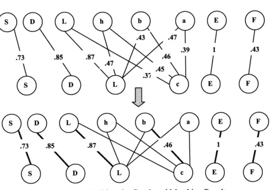
The next step is to create a bipartite graph using the non-zero total similarity scores and run the bipartite matching algorithm. Figure 3-8 depicts the initial bipartite graph, with total similarity scores, and the matched bipartite graph where the red arcs are the final matched pairs.

L h aa

.43

.

4

p

6

Figure 3-8: Bipartite Graph and Matching Result

The paired nodes must now be verified by their topology. Because every output node depends on every input node in both graphs, it is clear the topology is the same. The total graph similarity score must now be calculated using equation 3-X. Again, the modified pattern matching algorithm only uses the magnitude similarity score and not the total similarity score.

0.97 + 0.96 + 0.86 +1+0.87+0.94

6 = 0.93

In this example the graph similarity score was above 0.9, and the clustering algorithm was not required. However, if the similarity requirement was raised to 0.95, the clustering algorithm would still find these two graphs to match. Figure 3-9 depicts the magnitude-difference plot, and it is clear that there are two distinct clusters. Let node x represent a 3-Point bending node, and node X a cantilever node.

1 E 1 .43 F .43 L h b a .85 .87 .46 DL C

Diff.= Logo(rna _{) -Log}

1o(Xmag)

-2 -1.5 -1 -0.5 0 0.5 1 1.5 2

Figure 3-9: Magnitude-Difference Plot

The centers and standard deviations for these two clusters are -0.135 +/- 0.005 and -0.0325 +/- 0.0175. The distributions do not overlap out to two standard deviations and their standard deviations are far below the 0.3 cutoff. Therefore, the clustering approach would classify these two graphs as a match.

Chapter 4

Integration Classification

4.1 Integration Models

4.1.1 iModels

Integration models, known as iModels in DOME, are used to link model

interfaces together. Model interfaces in DOME are linked together using an object known as a parameter mapping. If two parameters are mapped together, they will act like a single parameter. If a model interface's mapped parameter value changes, the parameter's value which it is mapped to also changes to the new value. Two types of parameter mappings are possible: mapping between common input parameters, and mappings between input and output parameters.

Therefore, the definition of an integration model contains two things. It contains a list of all the model interfaces it is mapping together, and the parameter mappings

between these interfaces. Each mapping must designate which two model interfaces and parameters in the interfaces it is linking together.

4.1.2 Graph-based iModel Template Definition

The proposed method for classifying iModels uses previous iModels as templates for parameter mapping. Like the template developed for model interfaces, a template which describes an integration model is required. This template will be called an integration template.

The template for a model interface used a graph-based definition, as described in chapter 3. A similar graph-based definition for iModel integration template was

developed. This graph again contains both nodes and arcs. The graph nodes are template graphs and the arcs represent mappings between nodes in the template graphs. However,

there are two key differences. First, the architecture can be much more complicated because multiple parameter mappings can exist between two interface templates. Second,

this attributed graph is not fuzzy. Each node is a single template fuzzy ARG and not a fuzzy set of graphs. The formal definitions, definition 4-1 through 4-3, for the integration template graph representation are presented below.

Definition 4-1: an integration template node is an interface graph as defined

previously: g ={n1,n,---,n,,...,nn; a,a 2,.--,a,,,}, where n,n2,-.ni,.. n isa

set of attributed interface graph nodes and {a1 ,a.... ai,...aml is a set of arcs.

Definition 4-2: An integration template arc ai connects an interface graph's node

gh(nj)to another interface graph's node gi(nk)and it is denoted by a, = (g (nj ), g (nk))

Definition 4-3: An integration template graph is a directed graph:

G ={ 1'9"*Igi,-- g,,--g;ai,a2--,ai,,---,a,,,, where

(gi,g21

attributed interface graphs and (a1,a2,...ai,...am} is a set of arcs.

4.2 Integration Classification Algorithm

4.2.1 Introduction

The integration classification algorithm does not need to be as strict as the model classification algorithm. Integration models can contain hundreds of models and have many different functions. For example, an integration template for an entire automobile might contain the models for its drive train. Another designer who is only interested in an automobile's drive train should still be able to use this integration template to map together the drive train models. Matching all of the models in an integration template is not necessary.

It is also not necessary to map together all of the objective matches. Science and engineering is always advancing and new models are constantly being developed. Any possible mappings which are identified should be communicated to the designer for final

review. This algorithm is not intended to be capable of making the final mapping decisions because the breadth of possible models is too great.

4.2.2 Algorithm Overview

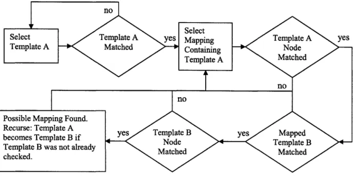
This algorithm is a recursive linear search. To begin, an integration template is chosen, and an interface template which the integration template maps together is chosen, this interface template will be referred to as Template A. The first step is to check if Template A. was matched to one of the objective interface graphs. If it was, it continues

by identifying all of the mappings to Template A. If it was not matched, the algorithm

begins again with the next interface template. After an interface template has been checked, it is flagged to ensure the algorithm will not repeat itself and fall into an infinite

loop.

The second step checks if the mapped node in Template A was matched to a node in the objective interface graph. The third step checks if the interface template, which maps to Template A, and will be referred to as Template B, was matched to an objective interface graph. The final step checks if the mapped node in Template B was matched to a node in its matched objective interface graph.

If any of the templates or nodes were not matched during the model classification

step, the algorithm will restart the process with the next mapping that includes Template

A. However, if they were all matched, the mapping is stored as a verified mapping. There

are two possibilities for how to proceed from here. If Template B has been flagged, the algorithm will check another mapping containing Template A. Otherwise, the algorithm will recurse and Template B will become Template A in order to check Template B's mappings.

no

IF _Select

Select Template A yes Mapping _{Template A yes}

Template A Matched Containing Node

Template A Matched

no no

Possible Mapping Found.

Recurse: Template A yes Templat B yes Mapped

becomes Template B if _{Node Template B}

Template B was not already _{Matched Matched}

checked.

Figure 4-1: Integration Classification Algorithm Flowchart

The key to this algorithm is that the mapped nodes in the template graphs were matched to objective interface graph nodes. If all of the mapped template nodes are unmatched, the integration template will be rejected and the next template will be checked.

4.2.3 Integration Algorithm Example

The following example will uses the procedure described previously for

integrating two models together. The intention of this example is to demonstrate many of the possible scenarios that can arise when attempting to map objective graphs using an integration model template. The models in this example do not bear any physical meaning. Figure 4-2 depicts the two bipartite graphs including the matched node pairs between the interface and template graphs. The attributed graph in figure 4-3 illustrates how the interface template graphs are mapped together in an integration model template. The mappings are represented by the bold red arcs.

Tem late A A B C E F a b c e f Interface a Tem late B L M N 0 W 1 m n o w Interface b

Figure 4-2: Matched Bipartite Graphs

--- I ---Template A Template Z D E C X Y W B v Z tv A L N K 0 Template B

The integration algorithm begins by choosing a template and checking if it is matched. Template A will be chosen first. As shown in figure 4-2, template A was matched to interface a. A mapping is then chosen which maps template A. The first mapping chosen will be the mapping between nodes A and K. Node A was matched to node a, in interface a, and the next step is to check mapped template, template B. Template B was matched to interface b, but node K was not matched during the bipartite matching. Therefore, this mapping is rejected.

The process continues by checking the mapping between nodes F and L. It was already found that template A was matched, and node F was also matched to node f in interface a. Node L belongs to template B which was already found to have been matched, but unlike node K, node L was matched to node 1 in interface a. This mapping is accepted and the integration model template is correspondingly accepted as a possible match.

The algorithm now recurses and begin the process again with template B. Again a mapping is chosen which maps template B. However, the mappings between template A and B are not eligible because template A has already been checked. If the algorithm were to return to template A, it could fall into an infinite loop. Thus the only remaining mapping is between nodes U and 0. Node 0 was matched to node o in interface b, but template Z was not matched to any of the objective interface graphs and the mapping is rejected.

All of the mappings involving template B and templates other than template A have been

checked, the algorithm now returns to template A. One final mapping remains between nodes G and M. Node G was not matched to a node in interface a, and the mappings is

rejected. All of the templates have now been checked and process is finished. In this example, the only accepted mapping is between nodes F and L.

Chapter 5

Direct Method

5.1 Introduction

Technology is always evolving, and the modeling of these technologies evolves as well. If integration of these new models is required, using previously built models as a

guide for parameter mapping would not be possible. Another method is needed which is capable of recognizing similarities within the objective models themselves.

Mappings merge two parameters into a single entity. It would seem reasonable to assume that before the mapping occurs, the individual parameters would be extremely similar-using the similarity measures described previously to assess that similarity. Input parameters from two interfaces can be compared, and input parameters from one interface can be compared to output parameters from a different interface. Unfortunately, it is not that simple because many parameters can be very similar but still should not be mapped together. This problem becomes very clear when considering CAD models that could contain hundreds of dimensions of similar magnitudes. This chapter will outline the logic and algorithm developed in order to identify only correct mappings.

5.2 Similarity Calculations

The first step is to calculate the similarity score between the nodes in all the objective graphs. Objective graphs are taken two at a time and the similarity scores for each combination of the input nodes of both models are calculated (input-input mapping), the similarity scores for all of the input nodes of the first graph and the output nodes of the second graph combinations (output-input mappings), and vice versa.

The similarity score is calculated in the same manner as described in section 3.2.2. Two separate similarity scores are calculated. One score only includes the magnitude

similarity calculation, and the second score includes the magnitude, unit, and name.

Each set of similarity scores, input-input and input-output, are run through the bipartite matching algorithm described in section 3.2.3.3. The optimal combination of nodes is found for both the possible input-input and output-input mappings.

5.3 Output-Input Mappings

Simulation models can be combined to operate in parallel or in series. When models operate in series, integrated simulations become very advantageous. Outputs from an initial independent model can be inputs for a subsequent dependent model. Multiple initial models might run in parallel to calculate inputs for the subsequent model. Generally these initial models are independent and mappings between them would not exist. However, a simple example of parallel models which would have common input parameters would be a CAD model and an accompanying cost model. Therefore, this method must be able to distinguish between these two cases. This can be accomplished

by identifying the output-input mappings first in order to determine which models are

independent and which dependent.

The process of identifying the output-input mappings is a basic linear search. The first pair of models is chosen and it determines whether or not the pair contains any possible input-output mappings. If it does, the algorithm begins to iterate through all of the possibilities, otherwise the next model pair is chosen.

The input node from the possible output-input mapping is identified. An input node can only be dependent on a single output. Therefore, the output-input mapping to a

given input node with the highest similarity score is chosen. Another linear search is performed to find the output-input mapping which maps to the identified input node with the highest magnitude similarity score. Only the magnitude similarity score is used because the name similarity score is too relative. The algorithm will only accept the

mapping as final if the mapping with the highest magnitude similarity score exceeds 0.9, indicating the difference in the node magnitudes is within one order of magnitude. During this search, every output-input mapping that maps to the identified input node is flagged to indicate it has been processed and will not be considered again.

5.4 Input-Input Mappings

Mappings between common input nodes can occur, but it is very difficult to accurately identify them. It is the intent of this thesis to aid in the integration of

simulation models. Incorrectly identifying mappings creates more work for the user and could eliminate any time savings. This problem will be avoided by requiring extremely high similarity scores for input-input mappings to occur.

The purpose of implementing the output-input mappings first was to understand the overall causality of integration model. In other words, to determine which models are dependent and which are independent. This is important because input parameters that

share a common dependent output parameter are less likely to map together. The probability that the two models are completely independent and calculate significantly different quantities is very high. Therefore, recognizing input parameters which share common dependent output parameters is crucial for eliminating incorrect mapping identification.

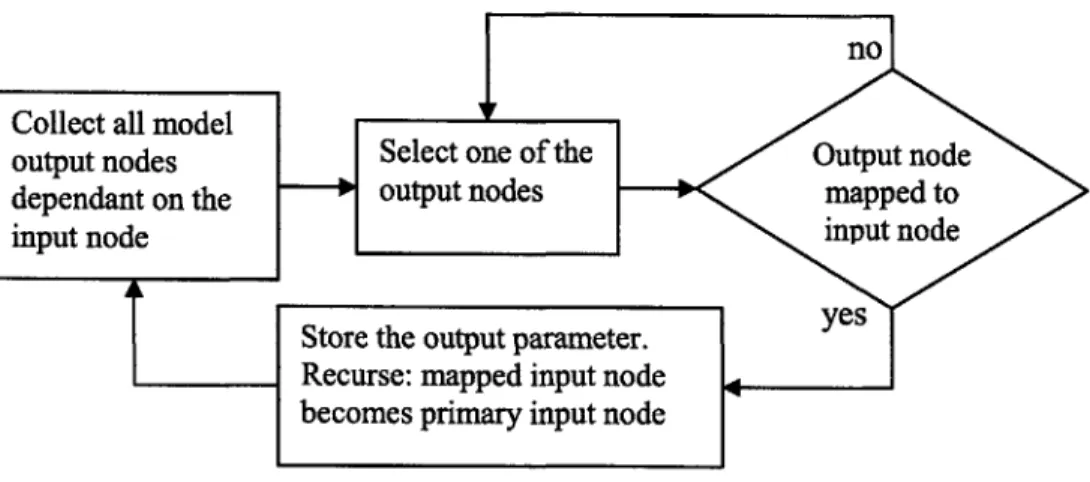
The algorithm that determines whether or not two input parameters or nodes share a common dependent output parameter is yet another recursive search algorithm. The algorithm traces the causality tree for one of the input parameters and collects all of the output parameters which depend on it. The same process is repeated for the second input parameter except when an output parameter is discovered that also depends on the first input parameter the algorithm stops. Figure 5-1 depicts the flowchart for the causality-tracing algorithm.

no Collect all model

output nodes Select one of the Output node

dependant on the output nodes mapped to

input node input node

Store the output parameter. yes Recurse: mapped input node

becomes primary input node

Figure 5-1: Causality Tracing Algorithm Flowchart

The two types of input-input mappings which can occur can now be separated from each other. Each type is required to meet a different heuristic. Possible input-input mappings which share a common dependent output parameter must have a magnitude

similarity score higher than 0.98 and all other input-input mappings must have a magnitude similarity score higher than 0.95.

5.5

Direct Method Example

The following figures illustrate the process the direct method algorithm would follow to map together three simple models for calculating the heat transfer in a pipe. Figure 5-2 depicts the problem and figures 5-3 through 5-5 depict each model graph.

tr