Automatic detection of research interest using topic modeling

Automatic Detection of Research Interest Using Topic Modeling

by

Rusmin Soetjipto

S.B., EECS

MIT 2004

Submitted to the Department of Electrical Engineering and Computer Science

in Partial Fulfillment of the Requirements for the Degree of

Masters of Engineering in Electrical Engineering and Computer Science

at the

MASSACHUSETTS INSTITUTE OF TECHNOLOGY

September 2013

© 2013 Massachusetts Institute of Technology. All rights reserved.

A u th o r ...

...

Department of Electrical Engineerin and Computer Science

September 9, 2013

Certified by ...

...

Prof. Regina Barzilay

Thesis Supervisor

A ccep ted b y ...

Prof. Albert R. Meyer

Chairman, Master of Engineering Thesis Committee

Automatic Detection of Research Interest Using Topic Modeling

by

Rusmin Soetjipto

Submitted to the Department of Electrical Engineering and Computer Science

September 9, 2013

in Partial Fulfillment of the Requirements for the Degree of

Masters of Engineering in Electrical Engineering and Computer Science

Abstract

We demonstrated the possibility of inferring the research interest of an MIT faculty member

given the title of only a few research papers written by him or her, using a topic model

learned from a corpus of research paper text not necessarily related to any faculty members

of MIT, and a list of topic keywords such as that of the Library of Congress. The topic model

was generated using a variant of Latent Dirichlet Allocation coupled with a pointwise

mutual information analysis between topic keywords and latent topics.

Thesis Supervisor: Regina Barzilay

Title: Associate Professor

Acknowledgements

First, I would like to thank my thesis advisor, Prof. Regina Barzilay, for her inspiration and kind support, without which this thesis project would never happen. I also would like to thank my academic advisor Prof. Rajeev Ram, my mentor and friend Tony Eng, as well as everyone in the Course VI Undergraduate Office for their generous guidance and assistance, which made it possible for me to return after more than seven years of Leave of Absence, and to complete my MEng degree.

I am very grateful for everyone in the Natural Language Processing and the Machine Learning research group at MIT CSAIL. Each one of you has been such a great support to me, not only in technical matters, but also by being a great friend.

Ika, you have kept me sane and alive throughout this entire year in MIT. I'm so grateful to have you as my best friend.

I dedicate this thesis to my parents, who were instrumental in my returning back to MIT. I also thank Cherrie, as well as her friends here in MIT and Boston, who has been kind enough to adopt her brother not only as her stand-in, but also as a good friend. I am really thankful for the MIT Graduate Christian Fellowship, Park Street Church's International Fellowship, as well as the members and honorary members of the Indonesian student community in MIT. You all have been my family away from home.

There are still so many others, which I have not mentioned, whose friendship and support have been so invaluable to me.

Last, but most importantly, I thank my God who has provided me with all these wonderful people, and also for revealing the secret of his wisdom and knowledge to mankind. If creating a machine learning algorithm takes no less intelligence than crafting hand-coded rules, then the theory of evolution should not make the universe be less intelligently designed either.

Contents

1 Problem Background 11 1.1 Data Sources 11 1.2 Baseline Method 13 2 Project Overview 17 2.1 Overall Strategy 17

2.2 Generating Topic Model 23

2.3 Inferring a Faculty Member's Topic 29

2.4 Finding Representative Topic Names 32

3 Further Details 35

3.1 Similarity Measures 35

3.2 BCEB-LDA 37

4 Results and Conclusions 45

4.1 Topic Model Result 45

4.2 Comparison with Baseline Method 45

5 Related and Future Work 59

5.1 Related Work 59

5.2 Possible Future Work 60

List of Figures (Including Tables)

Figure 1 - The true research areas of interest of some MIT faculty members, as well as those

predicted by the baseline m ethod ... 14

Figure 2 - Overall process of this thesis project... 18

Figure 3 - Plate diagram of BCEB-LDA... 43

Figure 4 -Sample entries from a generated Topic Model... 46

Figure 5 -Sample entries from a generated Topic Model (continued) ... 47

Figure 6 -Sample entries from a generated Topic Model (continued) ... 48

Figure 7 -Sample entries from a generated Topic Model (continued) ... 49

Figure 8 -Sample entries from a generated Topic Model (continued) ... 50

Figure 9 -Sample entries from a generated Topic Model (continued) ... 51

Figure 10 -Sample entries from a generated Topic Model (continued)...52

Figure 11 -Sample entries from a generated Topic Model (continued)... 53

Figure 12 -Result Comparison with Baseline Method...54

Figure 13 -Result Comparison with Baseline Method (continued)...55

Figure 14 - Result Comparison with Baseline Method (continued)...56

Chapter 1

Problem Background

The MIT Collaboration Graph Browser system is an internal MIT website that allows users to search for a faculty member's research information. This information includes among other things: his / her research areas, full-text data of research papers that he / she has authored, as well as the strength of collaboration relationship between him / her to other MIT faculty members. In this thesis report, we are focusing on the first item above, namely how we can improve the accuracy of the result that the system displays whenever a user queries the research areas of a particular faculty member. The proposed solution involves a novel application of a modified Latent Dirichlet Allocation model introduced by Branavan, Chen, Eisenstein, and Barzilay (2008), which will be referred to as BCEB-LDA in the rest of this thesis report.

1.1 Data Sources

In order to compute a faculty member's research area, the system has at its disposal several data sources.

First, we have obtained research paper bibliography and full-text data of each faculty member. This data, however, suffers from name ambiguity problem. For example, data on MIT CS & Al Lab's Robert C. Miller would also include research papers authored by other Robert C. Miller-s, including one that is affiliated with Mayo Clinic Research. This data source will be referred to as the non-disambiguated full-text data.

information (journal name, volume / issue, year, article title, etc.), and contains neither the abstract nor the full text of any research paper. Furthermore, the data source only covers a small proportion of a faculty member's entire research work. For example, out of 50+ research papers that Regina Barzilay has currently published during her career in MIT, only three research papers appear to be published by Prof. Barzilay in the data source. We will

refer to this data source as the disambiguated bibliographical data.

Third, we have obtained from the Library of Congress (LOC) online system a list of all keywords that it uses to categorize its collection of books and medias. These keywords range from general keywords such as "computers" to specific keywords such as "compilers" and "automatic speech recognition". We refer to this data source as the list of LOC areas.

Finally, for many of the research papers in the non-disambiguated full-text data above, we have also obtained from the LOC online system, the category keyword of the research journal that contains the said research paper. We will refer to this data as the LOC areas of a research paper. For example, the research journal "Artificial Intelligence in Medicine" is labeled with the keyword "Artificial Intelligence" by the LOC online system. Therefore, we say that the LOC area of all research papers that are published in this journal is "Artificial Intelligence".

Note that not all of the LOC areas tagging of documents are detected by the interface between our system and the Library of Congress data, due to difference in spelling or abbreviation of research journal names between our database and theirs. Consequently, only a subset of the research papers in our data (e.g. slightly less than 30% for the non-disambiguated full-text data), have their LOC areas identified. Moreover, even though some of the research journals may be tagged with more than one LOC area, the areas that a document is tagged with are almost always too few to represent the actual scope of area of

the said research journal. In the above example, we also found that the research journal "Artificial Intelligence in Medicine" is only tagged with the LOC area "Artificial Intelligence", even though it is reasonable to also relate this research journal with other entries in the list of LOC areas, such as "medicine" or "medical sciences".

1.2 Baseline Method

Previous approaches have been quite successful in capturing the research areas of each MIT faculty member, given the available data at the time (all the above data sources, minus the disambiguated bibliographical data). For each faculty member a, this original system returns all LOC areas 1, whose scorea(a, 1) value exceeds a certain threshold value. The scorea function measures how related a faculty member is to a certain LOC area, and is defined as:

( ZpEpaper(a) 1(LOCarea(p) = 1)

I

paper(a) 1 (1)

Here, paper(a) is the set of all research papers that is authored by faculty member a, while ll(LOCarea(p) = 1) is an indicator variable that returns 1 if the LOC area of paper p is 1, ane zero otherwise.

However, the result that is returned by this original system suffers from three problems: lack of coverage, area generalization, and name ambiguity. To better illustrate these problems, we have shown in Figure 1, the search results associated with some selected MIT faculty members, as well as their true research areas of interest (either as stated in their personal website or as commonly known by people in the MIT community who interact with them regularly).

The first problem stems from the fact that only a small proportion of research papers in our data source have their LOC area identified, as we have previously explained. In the case of

Edmund Bertschinger, our current Head of Physics Department, only one of his research papers has its LOC area identified. Consequently, a search on Prof. Bertschinger's research area only returns one LOC area.

Name True Research Areas of Interest Search Result (Baseline Method)

Edmund * Gravitation e Nuclear physics

Bertschinger

* Cosmology

e Large-scale structure

- Galaxy formation

* Relativistic accretion disks * Computation

Saman - Compilers optimization - Computers Amarasinghe

* Computer architecture - Electronic data processing 0 Parallel computing - Information storage and

retrieval systems

* Software engineering - Electronic digital computers * Microprocessors

0 Microcomputers Robert C. Miller * Crowd computing * Physics

* Online education - Science * Software development tools * Technology

e End-user programming _{* Biochemistry}

(and many more...) Figure 1 - The true research areas of interest of some MIT faculty members,

Prof. Bertschinger's research paper just described above, also illustrates the second problem, namely area generalization. The said research paper, titled "Prescription for successful extended inflation", is published in the "Physics Letters B" academic journal, which specializes in nuclear physics, theoretical nuclear physics, experimental high-energy physics, theoretical high-energy physics, and astrophysics. Although this research paper is mostly related to inflationary universe and hence astrophysics, it is assigned to the LOC area of the "Physics Letters B" research journal, which is nuclear physics. Astrophysics is indeed very closely related to nuclear physics, as many studies in astrophysics are concerned with the nuclear fusion reaction inside the core of a star. However, using "nuclear physics" as the sole LOC area label for this research paper or Prof. Bertschinger's research area in general, would risk misleading people into associating Prof. Bertschinger with nuclear reactors or atomic bombs, instead of cosmology or galaxy formation.

This problem of area generalization stems from the fact that a research journal usually contains several specialization areas and because the Library of Congress only assigns a few LOC area for this research journal, it must inevitably assign the LOC areas that are general enough to be the common denominators over all of the specialization areas that are covered by the research journal. This problem can also be seen in the case of Prof. Amarasinghe, where the search result of our baseline method tend to pick general LOC areas, such as "computers", which are not very useful for the intended user of the Collaboration Graph Browser system.

Lastly, we have the problem of name ambiguity, which has been explained in our introduction on the non-disambiguated full-text data. As evidently shown in Figure 1, the search result for Prof. Miller has been diverted away from the field of Computer Science

altogether by research papers in our non-disambiguated full-text data that correspond to the other Robert C. Miller-s.

Note, however, that the search results presented here does not exactly match those displayed by the Collaboration Graph Browser system. In this thesis report we are mainly concerned with the "raw" search result of an individual faculty member. On the other hand, when a user queries the research area a particular faculty member in the Collaboration Graph Browser system, the latter aggregates the "raw" search result of this faculty member with the "raw" search results of other faculty members who are collaborating closely with this faculty member, and then displays the top-ranked research areas of this aggregate search result. While the error that is caused by the aforementioned three problems is mitigated by this final processing stage, it is far from being eliminated.

Chapter 2

Project Overview

As previously shown, most of the problems suffered by our baseline method are rooted in our reliance on the Library of Congress' assignment of research journal to LOC area, which not only has limited coverage (due to difference in spelling or abbreviation of journal titles), but also tends to pick general LOC areas such as "computers" or "physics". In this thesis project, we propose a novel method of detecting a faculty member's research area that doesn't rely on the said manual assignment above. Furthermore, our method is able to utilize the strength of both the non-disambiguated full-text data and the disambiguated bibliographical data, while at the same time minimizing the effect of their weaknesses (i.e. ambiguity in the former, and the lack of full-text data in the latter). Figure 1 illustrates the overall strategy of our method.

2.1 Overall Strategy

First, we process both the list of LOC areas and the non-disambiguated full-text data to produce a topic model, using the BCEB-LDA algorithm. In effect, we "softly" split the collection of documents (i.e. research papers) into K different sets (where K is an integer parameter that is set manually), clustering documents with similar frequency distribution of words together (for example, it might find that many documents have high occurrence of the word "stimuli" or "neurons", but low occurrence of the word "unemployment" or "Keynesian"). For each set (i.e. topic), the algorithm then infers the topic's conditional language model (i.e. probability distribution of all the words in the vocabulary, as observed in the documents belonging to this set), as well as all the LOC area names that are

representative of this particular topic. Note that the splitting of the document is done "softly", which means that a document does not necessarily have to entirely belong to just one topic. Part of the document could belong to one topic, and other parts of the document to other topics.

Here, we assume each document as a bag of words, where each word v in the document is generated by a memoryless random process, independently from the words preceding and succeeding it (or any other words in the document for that matter), and independently of the order / location of the said generated word inside the document. This random process generates a word with a probability distribution P(vlk) that depends on the topic of the

Topic Model

Full- Prior Language Model LOC Area Names Text P("subjects"l1)= ... *Cognitive

P(k-1) P("response"I1)= ... neuroscience Data

... P("stimuli"|1) = ... *Motion perception

0: ... *Neural circuitry

List of P("language"12)= ... *Automatic speech Output LOC P(k=12) P("speech"112) = ... recognition

Areas ... P("word"112) =... *Computational

... linguistics

eSentence Fusion for Multidocument News Summarization" eAI's 10 to Watch

eModeling Local Co-S

herence: An Entity- 0

Based Approach *..

Disambiguated C

Bibliographical Data (Observed Data) Figure 2 - Overall process of this thesis project

said document (or to be exact, part of document), which we call k. This probability distribution P(vlk) is none other than the aforementioned conditional language model.

In concrete terms, the said topic model consists of:

(a) The a priori probability distribution, P(k) of all topic k, which is higher for a more common topic than that for a less common topic

(b) The conditional probability P(vIk) of all words v in the vocabulary given any particular topic k

(c) A set of LOC area names that best represents each topic v

Note that in order to make the computation of this topic model feasible, not all of the words in our non-disambiguated full-text data are included in the final vocabulary V. The methods employed to generate this final vocabulary and the said topic model will be discussed later in this section.

In all fairness, items (a) and (b) above can be computed even with a simple Latent Dirichlet Allocation (Blei, Ng, & Jordan 2003), and item (c) can then be determined, for example, by examining how similar the documents that are tagged by a particular topic are, with the documents that are tagged with a specific LOC area. However, BCEB-LDA is superior to this method in at least three ways:

(a) The topic inference and the "soft" assignment of documents (i.e. research papers) to topics is driven not only by the word tokens in the document's text, but also by the LOC areas that are tagged to each of the documents. The simple LDA model, on the other hand, does not use the latter.

(b) The result of BCEB-LDA already includes the joint probability (and hence likelihood) of a particular LOC area being assigned to a topic, as well as how likely any two LOC areas are referring to the same topic, while the result of simple LDA model includes neither of these, and hence requires a separate calculation of this joint probability (or likelihood) using a method that is not integrated into the Bayesian generative

(i.e. LDA) model.

(c) BCEB-LDA tolerates incomplete tagging information, by making use of the lexical similarity data. For example, even if a document is only tagged with the LOC area "Computational linguistics" and not "Natural language processing", the word tokens in this document still contribute to the generation of language model for the topic associated with "Natural language processing" (even if these two LOC areas end up being in different topics), because "Computational linguistics" and "Natural language processing" are lexically similar. On the other hand, the basic LDA model does not offer this level of robustness.

After the topic model is generated, we use it to infer the most likely topic for each faculty member a, by observing the research paper titles in the disambiguated bibliographical data that are associated with a, which we will refer to as the observed data. In other words, we calculate the likelihood of each topic k, given the observed data Da (list of all word tokens in the research paper titles associated to faculty member a) that remains constant across all topic k:

P(ktDa)OC P(k)

7

P( I k) (2)

VEDa vEV

We then choose a few topics (i.e. values of k) that maximize the value of the right hand side formula and consequently the left hand side formula as well, since the proportionality constant (i.e. normalization constant to make sure P(k

I

Da) sums to one) is positive. In

other words, we perform maximum likelihood estimation. Finally, the LOC area names that best represent these chosen topics are output as the research areas of faculty member a.

Since we only iterate v over the word tokens that are both in Da and in V, we are disregarding those word tokens in the research paper titles that are not part of the vocabulary.

In the general usage of language models, disregarding words that are not part of the vocabulary, like what we just did, will cause a disastrous error in the maximum likelihood estimation. By disregarding a word V^ in the observed data, we're in effect treating its conditional probability P('

I

k) to be one. It poses two problems. First, it violates the requirement that the conditional probability have to be normalized (the sum of the conditional probability across all words must sum to one). Second, it assigns the highest possible value that a conditional probability can take (i.e. one) to a situation that should have received a very low probability instead. For example, when calculating the joint probability of the English language model and some observed data that contains the word "sur", we cannot simply disregard the word "sur", which effectively assigns the word with conditional probability of one. In doing so, we end up assigning a higher conditional probability of "sur" (i.e. one) to the English language model than to the French language (whose vocabulary contains the word "sur", and hence assign the word "sur" some probability value that is certainly less than one), which is exactly the opposite of what we actually want. A normal practice in computational linguistic is therefore to assign a very low probability e to unseen words in the vocabulary (lower than the probability of any seen words). This is usually done through smoothing.

In the topic model like the one that we have, however, the language model of each topic has exactly the same set of words in the vocabulary, differing only in their frequency and hence

probability distribution. Therefore, a word in a data that is not part of the vocabulary of a topic's language model will not be part of the language model vocabulary of all the other topics either. Common sense dictates that we should assign a very low value E as the conditional probability of this unseen word when calculating the joint probability P(Da, k) of the observed data and a particular topic k. Therefore, if there are n words in the observed data that is not in the vocabulary, then for each topic k, the joint probability P(Da, k) will have the factor e' to account for these n words. However, since this factor is common to all of the topics (as all the other topics also don't have these n words in their vocabularies either), and since this factor is positive, we can simply disregard this factor of El altogether as we are only interested in the relative value (as the proportionality symbol in equation (2)

reminds us) of P(Da, k) across k, when calculating the likelihood P(k

I

Da).

Finally, we must also be aware of the limitation on how fine of a granularity that this topic model can achieve. As has been shown by Figure 2, our current topic model is not yet able to separate between "automatic speech recognition" and "computational linguistics" into different topics, even though these two LOC areas correspond to two separate research groups in MIT. In order to make our topic model robust in light of this limitation, we assign several LOC area names to each of the topic in our topic model. In the ideal situation, we would assign one LOC area name for each topic, and assign several topics to a faculty member. However, our model's limitation forces us to assign only a few topics (usually one topic) to a faculty member, each topic being represented by several LOC area names. Consequently, our algorithm will often output the same research area names for two faculty members, if their true research areas of interest are very similar. This may be reminiscent to the problem of area generalization that plagued our baseline method, and in fact, our new method also suffers from the same problem. However, the extent of the area generalization problem in our new method is much less than that in the baseline method. The fields of

"automatic speech recognition" and "computational linguistics" are much more closely related to each other than "astrophysics" and "nuclear physics". In our new method, the LOC area names that are clustered into the same topic as "Astrophysics" are all astrophysics-related LOC area names, such as "Extrasolar planets", "Telescopes", and "Cosmic rays".

One possible extension of this research is to see whether a hierarchical LDA (Blei, Griffiths, & Jordan, 2010) can be incorporated into the BCEB-LDA model. Even after we filter out stop words and general LOC areas such as "computers" and "physics", the more general words and LOC areas that remain might still give too much "distraction" that hinders our BCEB-LDA model from putting more "weights" on the more specific words and LOC areas to infer a topic model with a finer granularity. Integrating hierarchical LDA into our BCEB-LDA algorithm should improve its ability to neutralize the effect of those general words and to achieve finer granularity of topics.

2.2

Generating Topic Model

The previously mentioned topic model is generated using three input data:

(a) A list of all possible (research) area names

In our project, we are using the list of LOC areas. Alternatively, we can use data from another library (for example the MIT engineering library) or even a manually

crafted list, in order to better fit the specific domain that we're interested in.

(b) A full-text corpus that satisfies certain requirements

First, the corpus must be either the observed data itself (in our case, the research paper titles in the disambiguated data), or another data of a similar domain. As the disambiguated bibliographical data is too small (due to lack of full-text data and

serve as our full-text corpus. Both the disambiguated bibliographical data and the non-disambiguated full-text data are of similar domains (research paper titles vs. research paper titles and full text), which means that the language models (probability distribution over all words in the vocabulary) and hence the conditional language models (given any particular topic) would likely be similar for both data. This similarity of conditional language models is essential to produce a high-quality topic model.

The second requirement is that each of the possible research area names as mentioned in item (a) above, appears at least once in this full-text corpus. Area names that never appear must be discarded.

Lastly, we require that an area name related to a certain topic is more likely to appear in a document (i.e. research paper) that is related to that topic than in a document that is not. This is one of the basic characteristics of any intelligible writings, and hence can be safely assumed to also be true of our full-text corpus.

Note that we do not require that the full-text corpus be disambiguated. In fact, we do not even require any author-to-document attribution at all. Had the non-disambiguated full-text data not been available, we can simply substitute it with other full-text corpus of similar domain, such as research paper full-text data from other universities or public repositories such as arxiv.org, or even article full-text data from Wikipedia.

(c) A parameter K, which sets the number of topics in our topic model

This parameter is an input to the BCEB-LDA algorithm (which we are using to generate the topic model), and is manually tuned in order to achieve the best

performance of our topic model. When K is set too low, the topic model will clump together topics that could have potentially be separated out from each other, hence not reaching as fine granularity of topics as it potentially could. However, when K is set too high, the model breaks down altogether and start assigning topic to (research) area names that are not at all related to the topic. We have found that setting the value of K between 70 and 75 is optimal given our particular full-text corpus.

A possible extension of this project is to develop a non-parametric version of the BCEB-LDA algorithm, using a hierarchical LDA (Blei, Griffiths, & Jordan, 2010) for

example. A non-parametric BCEB-LDA would no longer require the parameter K as input, and instead would automatically infer K.

Note that for simplicity sake, we have disregarded many other parameters in the BCEB-LDA. These parameters (such as Dirichlet priors) are "soft" in a sense that misadjusting them would bring significant impact to neither the result nor the performance of our algorithm, except if it is misadjusted by factors of magnitude (e.g. misadjusted by a factor of 100x or more). We found that BCEB-LDA in its default settings performs well on our task. Further details of these parameters are explained by Branavan et al. (2008).

The first stage of this topic model generation process is to tag each document with all LOC areas whose name appears verbatim in the text of the said document. A document containing the word "computer architecture", for instance, will be tagged by the LOC area "computer architecture" but not "computers" (unless the word "computers" in its plural form also appear on the document text). If a pair of LOC areas is tagged to a document, but the name of one area is a substring of the other area's name, then only the latter is used to

tag the document. For example, the list of LOC areas also includes the area name "architecture", but our aforementioned example document is not tagged with the LOC area "architecture", because it can also be tagged with "computer architecture". In other words, we are only tagging document with area names that are the longest substring of the

document text. Note that the name for each LOC area is not unique. For example, there are two LOC areas with the name "membranes". In order to disambiguate them, a different

qualifier term is tagged by the Library of Congress to each of the areas with ambiguous name. In the case of "membranes", one is tagged with the qualifier term "biology", and the other with the qualifier term "technology". For all LOC areas with ambiguous names such as these, we only tag a document with such a LOC area if and only if both the area name and its qualifier term exist in the document text. Therefore, a document would only be tagged with LOC area "membranes" of the biological variety if and only if such document contains both the word "biology" and the word "membranes" in its text.

In the second stage, we filter out LOC areas with document frequency (i.e. the number of research paper document that is tagged with a particular LOC area) that is too high (which indicates a too general LOC areas such as "computers" or "physics" that are not relevant to our intended users) and LOC areas with document frequency that is too low. After some experimentation, we found that in our specific case, we obtain the desirable level of area specificity when we discard about 20% LOC areas with the most document frequency, and about 50% LOC areas with the least document frequency, out of all LOC areas that has been successfully tagged to at least one document. We refer to the final result of this filtering

process as the reduced LOC area list.

In the third stage, we filter out words that are less than 3 characters, words that are more than 20 characters, and words that contains too many digit characters (i.e. words whose

digit characters make up more than 20% of the word's total characters). Then, we filter out about 75 words that occur most often in the remaining pool of words. Due to the size of our full-text corpus, this method successfully removes all of the stop words (e.g. "the", "this", "since") without any supervision data, as well as other common words, which is usually not subject specific. The conditional probability of these words does not vary much across different topics and hence does not much improve our algorithm ability to distinguish one topic from another. Finally, in order to achieve a reasonable computation time of BCEB-LDA, we filter out all the words that occur the least often until we have reached a vocabulary size that provides a good balance between computation cost and quality of result. In this project, we found that a vocabulary size between 7500 and 10000 word types provides such balance. Note that the vocabulary that is used to compute the lexical similarity matrix (as will be explained below) is the same as the vocabulary that is used by the BCEB-LDA, short of this final step of size reduction. This is due to two reasons. First, the computation of lexical similarity matrix takes far less time than the BCEB-LDA algorithm even with the bigger vocabulary size. Second and most importantly, the quality of lexical similar matrix is greatly affected by the size of the vocabulary that is used when computing the said matrix.

While the determination of which LOC areas to filter out is based on their document frequency, the determination of which word types to include in the vocabulary is based on their token frequency. If the LOC area name "computer architecture" appears five times in a document, the LOC area is counted five times in the token frequency, but only once in the document frequency.

Note also that once a document is tagged by a certain LOC area, this document to LOC area connection is preserved, even if part or all of the word types that make up the LOC area name and / or qualifier term does not make it into our final vocabulary.

In the fourth stage, we calculate the lexical similarity and co-occurrence similarity of each pair of LOC areas in the reduced LOC area list. This calculation, which will be elaborated in section 3.1 of this thesis report, produces two symmetric matrices, one corresponding to the lexical similarity, and one corresponding to the co-occurrence similarity. The value of the i-th row of the j-th column of these matrices denotes the similarity (lexical similarity in the first matrix, and co-occurrence similarity in the latter) between the i-th LOC area and j-th LOC area.

The lexical similarity measures how similar the frequency distribution of words that "accompanies" a LOC area name is with that of another LOC area name. A word that "accompanies" a LOC area name is all the M words that precede a LOC area name, and all the M words that succeed it, every time such area name occurs in the text. (Of course, if a LOC area name begins near the beginning or end of a document, then number of words that "accompanies" it might be less than 2M.) In this project, we set the value of M to be 10.

The co-occurrence similarity between two LOC areas compares how many documents that are tagged with both LOC areas, versus how many documents are tagged with just one of them. The higher the former (in comparison with the latter), the more similar the two LOC areas are.

In the fifth and last stage of our topic generation process, we run the BCEB-LDA algorithm to produce our topic model. Several input data are fed into this algorithm, including:

1. The full-text corpus in the form of a matrix, where the value of the i-th row of the

j-th column is j-the number of times j-thej-j-th word in j-the (size-reduced) vocabulary appears in the i-th document (i.e. research paper) of the full-text corpus

2. A matrix that describes which LOC areas are tagged to each of the documents in the full-text corpus. The i-th row of the j-th column is one if the ]-th area in the reduced LOC area list is tagged to the i-th document is tagged with, and zero otherwise. Note that a document can be tagged with multiple LOC areas, and a LOC area can be tagged to multiple documents.

3. The parameter k that we have previously discussed

4. A (finalized) similarity matrix, which is computed by averaging the two similarity matrices computed in the fourth stage above, and by "smoothing" the resulting matrix as follows. If any cell value is less than 0.2, we replace it by 0.2, and if any cell value is more than 0.8, we replace it by 0.8.

Further details of the BCEB-LDA algorithm are explained in section 3.2 of this thesis report.

Finally, it's also worth noting that throughout the entire process above, we treat all words as case insensitive, except when they are in all-capital letters. For example we treat "aids",

"Aids", and "AiDS" to be of the same word type, but "AIDS" to be of a separate word type. Furthermore we discard diacritics, treating o and 6 to be the same, which might not be entirely accurate (for example, the standard conversion procedure for the German 6 is actually to turn it into "oe"). However, since most if not all of the research papers in our data are in English, this simplification will not introduce any significant problem.

2.3 Inferring a Faculty Member's Topic

Using the output of the BCEB-LDA algorithm, we can find the best estimate of several (marginal) probability distributions that are of our immediate concerns, namely:

(b) The conditional probability of all word v in the vocabulary, P(v

I

k), for all topic k

Both of which have been elaborated in section 2.1 above.

(c) The joint probability P(k, 1) of each topic k and each area 1.

Note that in (c) above, and in future references to LOC area, we are only concerned with LOC areas that are part of the final (reduced) list of LOC areas, as explained in section 2.2 above. We define L as the number of LOC areas in this final list.

Based on output (c) above, we calculate the Pointwise Mutual Information (PMI) between each topic k and each LOC area 1 using the following formula:

P(k,l)

PMI(k,

1)

= log _{P(k) P(1)}

P()

(3)

3 where P(k) = P(k, l) and P(1)= P(k, 1).

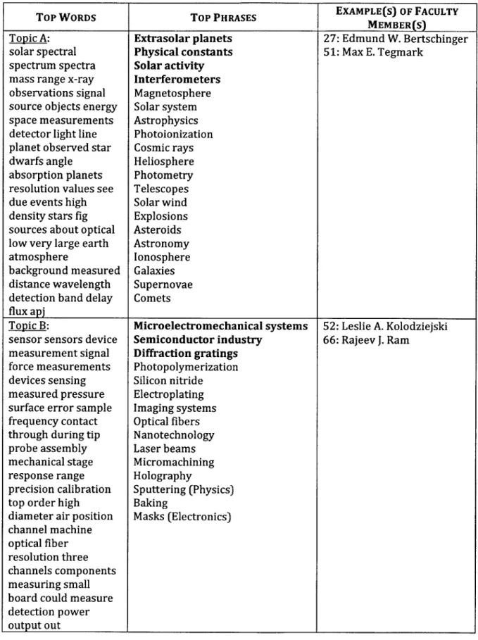
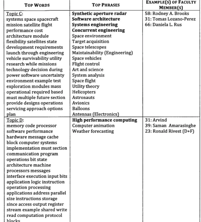
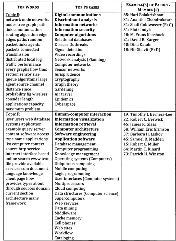
Each area 1 is then assigned to the topic that has the highest PMI with 1. Figure 4 to 11 shows some examples of topics along with the all the LOC areas that are assigned to these topics. The result in these figures corresponds to a BCEB-LDA execution with parameter k = 75. For each topic, we also list several words inside the vocabulary that has the highest conditional probability given the said topic.

Finally, using output (a) and (b), as well as the observed data (i.e. the research paper titles in the disambiguated bibliographical data), we infer the most likely topic for each of the faculty member, using the procedure explained in section 2.1 above. In Figure 4 to 11, we also show several faculty members that are assigned (based on this procedure) to each of the sample topics. There are a few details from the said inference procedure that have so far been omitted for simplicity's sake:

1. Topic that is not assigned to any LOC area will be disregarded. Note that in our observation, most of the topics (more than 97%) are assigned to at least one LOC area. Furthermore, if the parameter K is not stretched to its maximum limit, this proportion is almost always 100%.

2. Although we usually associate only one (i.e. the most likely) topic to each faculty member, in the rare instance where the likelihood of the second most likely topic is close in magnitude as that of the first topic (i.e. roughly 10% as likely, or more), we also include this second most likely topic as part of the faculty member's research areas. In Figure 4 to 11, if a faculty member is associated with more than one topic, we put his / her name on his

/

her most likely topic, and list his / her second most likely topic at the end of his / her name. For example, in Figure 6 we see that Nir Shavit's most likely and second most likely topics are topic E (networking, algorithms, security, etc.) and topic D (high performance computing) respectively.

3. Due to lack of coverage in the disambiguated bibliographical data, some faculty members have just two or even one research paper associated with him or her. If the overlap between the observed data (i.e. word types in the research paper titles for a particular faculty member inside the disambiguated bibliographical data) and the vocabulary is less than ten word types, we would use the non-disambiguated full-text data instead of the disambiguated bibliographical data as the observed data for the said faculty member.

Moreover, on top the data that we have listed in section 1.1, a disambiguated full-text data (in the form of grant proposal full-text) exists for a very small number of faculty members. When this data is available for a particular faculty member, we use this data instead of the disambiguated bibliographical data as our observed data.

In all of our figures and results, we only show faculty members whose observed data are the disambiguated bibliographical data (i.e. disambiguated research paper titles), and are substituted by neither the disambiguated full-text data nor the

non-disambiguated full-text data. To further show the robustness of our method, we have included in Figure 4 to 11 the number of word types in the overlap (as

previously mentioned) between the vocabulary and each faculty member's observed data. This number can be found on the left side of each faculty member's name.

2.4 Finding Representative Topic Names

As shown in Figure 4 to 11, the limitation of our topic granularity causes many LOC areas to be clustered into the same topic. However, displaying all of those topics in the Collaboration

Graph Browser system would only confuse our users. Therefore, several representative LOC area names need to be selected for each topic.

Ideally, the selection of these representative area names is done through a feature-based supervised learning, or other similar techniques. Some of the features that might prove useful include:

(a) The Point Mutual Information (PMI) between the said LOC area name and the topic under consideration, as defined in equation (3) above.

(b) The document frequency of the said LOC area

(c) The document frequency of the said LOC area name in relation with the entire (reduced) LOC area list. This can be in the form of a percentile for example, where the LOC area with the most document frequency assumes the value 100%, and the

LOC with the least document frequency assumes the value 0%.

Since shorter LOC area names tend to have higher document frequency than longer LOC area names, we can also replace feature (c) with a similar document frequency percentile, that is compared not against the entire LOC area list as explained above, but instead only against all the LOC area names that have the same number of characters as the LOC area name of interest.

A good supervised learning must take into account the fact that there is usually more than one right answer when choosing a good representative topic. Although not directly related to our present problem, Branavan, Deshpande, and Barzilay (2007) introduced an example

of such learning method that can be easily repurposed for our present problem.

The training data itself can either be curated from the faculty member's websites or CV, as well as from MIT's internal administrative record. However, the area names listed in these data sources might be slightly different than the LOC area names (e.g. a faculty might identify his / her research interest as "parallel computing" or "parallel architectures", while Library of Congress might uses the name "parallel computers" or "high performance computing" instead). Alternatively, training data can be obtained by asking respondents to rate the quality of the representative topic generated by our system (e.g. via Amazon Mechanical Turk) as demonstrated by Lau, Grieser, Newman, and Baldwin (2011). However, as their research shows, even the human annotators themselves does not completely agree with each other, as the average human annotator would only receive the score of 2.0-2.3 when his / her answers are scored by the others. Here, 2 means "reasonable" and 3 means "very good".

As good-quality training data is not yet available at the time of writing of this thesis report, and since the quality of user experience takes precedence over the research value of our method, we decided to use a simple heuristic method that has shown to be very satisfactory

for the particular problem domain that we are facing. We multiply a LOC area's PMI with respect to the topic of interest (feature (a) above), together with the number of characters in this LOC area name (feature (d) above), and use the product of this multiplication as the score of the said LOC area. The 20% of LOC areas with the highest score (rounded up) in a given topic are selected as the representative names for that topic. In Figure 4 to 11, we have sorted the LOC areas in each topic descendingly according to their scores, which are computed using the heuristic formula that we have just explained. The LOC area names that are chosen as representative names for each topic are shown in bold characters.

Chapter 3

Further Details

In this chapter, we briefly explain how the cosine similarity is calculated, and how BCEB-LDA infers the topic model. Readers who are familiar with these topics should proceed to the next chapter.

3.1 Similarity Measures

In section 2.2 above, we have computed the lexical similarity matrix and the co-occurrence similarity matrix between each of the LOC areas of our interest. The computation of these two matrices differs only in the features that are used to compute the joint distribution matrix (see (a) below). The overall computation itself is divided into three stages:

(a) Computation of joint distribution matrix

The result of this computation stage is a two-dimensional matrix of size L x F, where L is the number of LOC areas of interest, and F is the number feature. Here, the l-th row of the f-th column denotes the number of times feature f occurs in LOC area 1.

Further details of these features will be explained later in this section. Before proceeding to the next stage, the said matrix is divided by a normalization factor so as to make sure that the content of this matrix sums up to one, hence the name "joint distribution matrix". In other words, the l-th row of the f-th column of this final matrix is the joint probability of feature fand LOC area 1.

In this stage, a new two-dimensional matrix of size L x F is created. The l-th row of the f-th column of this matrix is the PMI between feature fand LOC area 1, which is defined as:

P(f,

1)

PMI(f, 1) = log P(f) P()

(4)

Here, P(f, 1) is the 1-th row of the f-th column of the probability distribution matrix, P(f) is the sum of the f-th column of the probability distribution matrix, and P(1) is the sum of the l-th row of the probability distribution matrix. Before proceeding to the next stage, all negative values are removed (i.e. replaced with zeroes), hence the name "positive PMI".

(c) Computation of the (cosine) similarity matrix

In this final stage, we create a symmetric two-dimensional matrix of size L x L. The 11-th row of the 12-th column of this matrix denotes the cosine similarity between

the 11-th LOC area and 12-th LOC area, which is defined as:

similarity,, (1i, 12) =

f{pMI (f, 11)} 2 . {f PMI U, 12 )J2

In other words, if we picture the 11-th and l2-th rows in the PPMI matrix as two

vectors of size F, then the cosine similarity between LOC area 11 and 12 is the dot product between these two vectors, divided by the product of their magnitudes, hence the name "cosine similarity".

As previously stated, the difference between lexical similarity matrix and co-occurrence similarity matrix lies only in the features that are being used for the above computation:

(a) The features used in the lexical similarity matrix are all the word types in the vocabulary. The number of times feature f occurs in LOC area 1 (i.e. the content of the I-th row of the f-th column) is the number of times a word of type f appears (in the full-text corpus) "near" the name word / phrase of LOC area 1. By "near", we mean that the said word of type f must not be separated from the LOC area name by more than M words. In this project, we set the value of M to be 10.

(b) The features used in the co-occurrence similarity matrix are all of the documents (or to be more exact, all of the document identifiers) in the full-text corpus. The number of times feature f occurs in LOC area 1 is simply the number of times the name LOC area 1 appears in document

f.

In our project, however, we slightly modify this co-occurrence similarity matrix, by replacing all values that are greater than one, with one.

Lin (1998) has given a good and detailed explanation about similarity matrices.

3.2

BCEB-LDA

This particular section requires background knowledge of the Bayesian generative model and Gibb's sampling. Koller and Friedman (2009), as well as Jordan (1999) provide a good introduction on the said topics. Alternatively, the reader may also continue to treat BCEB-LDA as a black box, just like what we have done in this thesis report up until this point.

The BCEB-LDA is an extension of Latent Dirichlet Allocation, and is a type of Bayesian generative model. In this model, we define the joint probability of several random variables that we think are relevant to the problem at hand. We then fix certain variables (which we refer to as observed variables) to some values (based on the observation / input data that we have). Next, we compute the joint probability of the remaining variables conditioned

upon the particular values of these observed variables. Finally, we reduce this joint probability to only include those variables that we are interested in. In other words, we find its marginal probability by summing this joint probability over those variables that is neither observed nor needed for our final result.

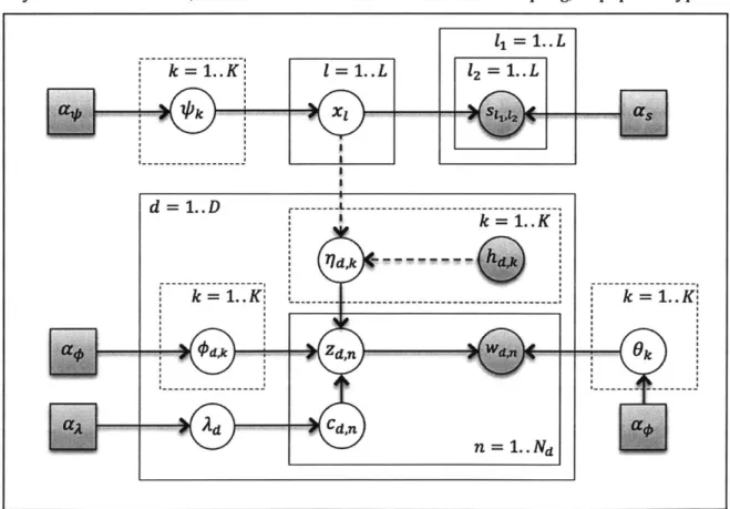
All the (random) variables that are relevant to our particular problem, are as follows:

(a) A continuous random vector variable

4

of size K (i.e. number of topics), whose components must sum to one and must each be a real number between 0 and 1. The k-th component of this vector denotes the a priori probability of a LOC area being assigned to the k-th topic (given no other data or observation). The probability distribution of this random vector variable follows a Dirichlet distribution, hence for all possible combination of non-negative vector of real numbers (1p₁, 2, ...,K) whose components sum to one:

K

PO(1

2,-

K

'

1

(6)

Za) k=1

Here, we use a variant of Dirichlet distribution with a symmetric prior. The normalizing factor Z(ap) = r(Ka ,) where F(x) = fo txletdt is the gamma

[r(agp)]"

function, makes sure that this probability distribution sums to one. Also note that we have chosen a Dirichlet distribution, because doing so will simplify our inference computation (as this distribution is the conjugate form / conjugate prior of a multinomial distribution), and not necessarily because of its accuracy in reflecting our belief about the true a priori probability of 4'.

Note the presence of the parameter ap above, which influences how "skeptical" the model is with the observed data. (A high ac means that the model is more willing to

consider unseen topics, even if all the observed data so far are concentrated in only a few popular topics). In this project, we set a* to be 0.1.

(b) For each LOC area 1, a discrete random variable x, that denotes the topic assignment of LOC area 1. The value of this random variable x, for each LOC area 1 is independent from those of the other LOC areas, and can take an integer value between 1 and K (inclusive). Each x, is drawn from the probability distribution that is described by the K-sized random vector variable 4 (see item (a) above). In other words, x, is dependent on

4.

(c) For each pair of LOC areas, l1and 12, a continuous random variable sl,12 that takes a

different probability distribution depending on the current value of x1 and xL1 (item

(b) above). In other words, s11,1, is dependent on xl1and xl1. The random variable

S1,1 takes the Beta(2,1) probability distribution if l1and 12 are assigned to the same

topic (i.e. x1l = x12), and the Beta(1,2) probability distribution if 11 and 12 are

assigned to different topics. In both cases, S11,12 can only take a real value between 0 and 1. In Figure 3, the hyperparameters of the above Beta probability distributions

(i.e. (2,1) and (1, 2)) are denoted as a.

The Beta distribution is simply a Dirichlet distribution with two dimensions, and hence one degree of freedom. In other words, for 0 < s₁₁,12 < 1:

S,2(1 _{- S11,12) if}

x 11 = X P(s, x) =(7)

S1,(1 - s₁₁,_{1 2})2 otherwise

Note that the value s11,12 for all pair of LOC areas are observed, since it must be set to the same value as the (finalized) similarity matrix that is fed as an input to our

(d) For each document d, a vector hd of size L that denotes the set of all LOC areas that document d is tagged with. The I-th component of the vector is one if document d is tagged with the I-th LOC area, and zero otherwise. This vector is an observed data, as it is simply the d-th row of the input matrix that contains the tagging information. (e) For each document d, a vector li of size K that is dependent on item (b) and (d) above. The k-th component of this vector is one if document d is tagged by at least one LOC area that is currently assigned to the k-th topic in item (b) above, and zero otherwise. Note that 17 is not really a random variable, as it is deterministically calculated from item (b) and (d) above. In other words, 17 is simply a derived variable from these other variables, and whose sole purpose is to facilitate our understanding of the BCEB-LDA generative process.

(f) For each document d, a continuous random vector variable

#3d

of size K that is similar to

4

in item (a) above. The k-th component of this vector, however, denotes the a priori probability of document d (instead of a LOC area) being assigned to the k-th topic. Each random vector variable bd for all document d takes a vector value according to the Dirichlet distribution similar to that explained in item (a) above, but with hyperparameter a, instead. In this project, we set this hyperparameter to

be 0.001.

(g) For each document d, a continuous random variable ad between 0 and 1 (inclusive) that denotes how likely it is for a word token in d's title and text to be influenced by the topic of a LOC area that is tagged to document d. The random variable Ad follows

a Beta(1, 1) probability distribution. In other words, for all 0 5 Ad < 1: 1

PA)= §td(1 -Ad)(8

2 (8)

(h) For each document d, a discrete random vector variable Cd of size Nd (the number of word tokens in d's title and text data). The i-th component in Cd is one if the topic of the i-th word token in document d is influenced by one of the LOC areas that are tagged to document d, and zero otherwise. In the latter case, the topic of the i-th word is influenced by the latent topic distribution bd of document d itself (item (f) above). All of the components in vector Cd are independent from each other, and are only dependent on the random variable Ad (item (g) above). Each component takes the value 0 or 1 with probability (1 - Ad) and Ad respectively.

(i) For each document d, a discrete random vector variable Zd of size Nd. The i-th component in Zd denotes the topic of the i-th word token in document d. Each component in this vector is independent from each other, and has a probability distribution that is dependent on the vector 17 (item (e) above), as well as the random vector variables 4

d and Cd (item (f) and 0 above). Each component in Zd can take an integer value between 1 and K (inclusive) with the following probability distribution:

e If the i -th component of Cd is zero, then it takes the integer value

between 1 and K with the probability distribution described by the random vector variable

#d

of size K described in item (f) above.

* If the i-th component of Cd is one, then it takes one of the topics that have non-zero value in 17 with equal probability.

() For each topic k, a continuous random vector variable 6_{k of size V (i.e. number of}

word types in the vocabulary). All of the components of this random vector variable must sum to one, and must each be a real number between 0 and 1 (inclusive). The i-th component of 0

k denotes the probability that a word token of topic k is of the same type as the i-th word type in the vocabulary. Furthermore, Ok assumes a

Dirichlet probability distribution with hyperparameter ao . Therefore, for all possible combination of non-negative vector (0;,, 6i,2, -.., Bi,V) whose components sum to one:

V

P0(6i,1, i,2 , = Z( 1) 6 ae-1

(9) Z~~)j=1

Again, Z(ao) = r(vao) is the normalizing constant to make sure the above

I[r(ae)Iv

probability distribution sums to one.

(k) Finally, for each document d, a discrete random vector variable Wd of size Nd, which is dependent on the random vector variable Zd as well as 6_{k (for all topic k) as}

described in item (i) and (j) above. The i-th component of Wd denotes the word type of the i-th word token in document d, and takes an integer value between 1 and V (inclusive) with the probability distribution described by the vector random variable Oj of topic

j,

where

j

is the value of the i-th component of Zd.

Clearly, the Wd is also an observed variable, as it must match the actual text document of our full-text corpus.

Note that in order to better explain the generative model above, we have slightly abused the definition of probability distribution to also refer to the probability density of a continuous random variable.

The plate diagram (Figure 3) above summarizes the generative process of our BCEB-LDA. Dashed lines denotes a deterministic generation of (derived) variable, while dashed plates indicates vector variables that usually are not denoted with plates in the traditional notation. Finally, D is the number of documents in our full-text corpus.

Given an infinite computing resource, we may simply multiply the probability or conditional probability of all the random / vector variables listed above, and since there are no circular

dependencies, we would get a joint probability of all of the relevant variables. We can then simply set the values of the observed variables according to our input data, and find the marginal probabilities of our interest, namely:

(a) The joint probability of topic and word token type (item (j) above).

(b) The joint probability of topic and LOC areas (item (b) above).

(c) Either the marginal a priori probability that a LOC area takes a particular topic (item (a) above) or the marginal a priori probability that word token (that is not influenced by a LOC area tag) of a randomly selected document takes a particular topic (item (0 above). In this project, we have decided to use the former.

However, since the above computations are not feasible even with the computing power in any foreseeable future, we resort to the method of Gibb's Sampling, a popular type of

- = 1 d =1..D -- ---L--- ---k = L..K: Cd,n n L=..Nd

Figure 3 - Plate diagram of BCEB-LDA

2 = 1.. L