Algorithm to calculate the Minkowski sums of 3-polytopes : application to tolerance analysis

(1)

HAL Id: hal-00694205

https://hal.archives-ouvertes.fr/hal-00694205

Submitted on 9 May 2012

HAL is a multi-disciplinary open access

archive for the deposit and dissemination of sci-entific research documents, whether they are pub-lished or not. The documents may come from teaching and research institutions in France or abroad, or from public or private research centers.

L’archive ouverte pluridisciplinaire HAL, est destinée au dépôt et à la diffusion de documents scientifiques de niveau recherche, publiés ou non, émanant des établissements d’enseignement et de recherche français ou étrangers, des laboratoires publics ou privés.

Algorithm to calculate the Minkowski sums of

3-polytopes : application to tolerance analysis

Denis Teissandier, Vincent Delos, Lazhar Homri

To cite this version:

Denis Teissandier, Vincent Delos, Lazhar Homri. Algorithm to calculate the Minkowski sums of 3-polytopes : application to tolerance analysis. 12th CIRP Conference on Computer Aided Tolerancing, Apr 2012, Huddersfield, United Kingdom. pp.84-90. �hal-00694205�

(2)

12

th

CIRP Conference on Computer Aided Tolerancing

Algorithm to calculate the Minkowski sums of 3-polytopes :

application to tolerance analysis

Denis Teissandier

a*

, Vincent Delos

b

, Lazhar Homri

a a Univ. Bordeaux, I2M, UMR 5295, F-33400 Talence, France.

CNRS, I2M, UMR 5295, F-33400 Talence, France.

Arts et Metiers ParisTech, I2M, UMR 5295, F-33400 Talence, France. b Univ. Paris Descartes, MAP5, UMR 8145, F-75270 Paris cedex 06, France.

Abstract

In tolerance analysis, it is necessary to check that the cumulative defect limits specified for the component parts of a product are compliant with the functional requirements expected of the product. Cumulative defect limits can be modelled using a calculated polytope, the result of a set of intersections and Minkowski sums of polytopes. This article presents a method to be used to determine from which vertices of the operands the vertices of the Minkowski sum derive and to which facets of the operands each facet of the Minkowski sum is oriented.

Keywords: Tolerancing analysis ; Minkowski sum ; polytope ; normal fan

1. Introduction

Minkowski sums can be used in many applications. Some of the most important ones that should be mentioned are for determining the envelope volume generated by displacement between two solids, whether in geometric modelling, robotics or for simulating shapes obtained by digitally controlled machining [1].

In geometric tolerancing Fleming established in 1988 [2] the correlation between cumulative defect limits on parts in contact and the Minkowski sum of finite sets of geometric constraints. For examples of modelling dimension chains using Minkowski sums of finite sets of constraints, see [3], [4], [5] and [6]. In tolerance analysis, it is necessary to check that the cumulative defect limits specified for the component parts of a product are compliant with the functional requirements expected of the product. Defect limits can be modelled by tolerance zones constructed by offsets on nominal models of parts [7]. Cumulative defect limits can be modelled using a calculated polytope, the result of a set of intersections and Minkowski sums of polytopes. A functional requirement can be qualified by a functional polytope, in other words a target polytope. It is then necessary to verify whether the calculated polytope is included in the functional polytope [8], see fig. 1.

To optimise the filling of the functional polytope (see fig. 1), it is crucial to know. - from which vertices of the four operands the vertices of the calculated polytope derive,

(3)

Functional 3-polytope Calculated 3 -polytope +

+

=

Functional 3-polytope Calculated 3 -polytope + +

+

++

=

Fig. 1. Verification of inclusion of 3-polytope [13]

The purpose of this article is to determine the Minkowski sum of 3-dimension polytopes and apply this effectively in order to optimise the filling of the functional polytope. Our approach is based on polytope properties, most of which are described in [9] and [10].

Several different approaches have been proposed in the literature to determine the Minkowski sum, most of which relate to 3-dimension geometrical applications.

For example, [11] improves the concept of slope diagrams introduced by [12] to determine facets of connection. The same principle is used by [13] who proposes an algorithm called a Contributing Vertices-based Minkowski Sum.

2. Some properties of polytopes

2.1. Two dual definitions for polytopes

A polytope  is a bounded intersection of many finitely closed half-spaces in some n (see fig.2) [10]. This is the h-representation of a polytope [14].

In this article, a system of inequalities for m half-spaces H has been chosen to define a polytope  as eq. 1:



A b,





x n:



with m n and m

   A.x b A b

     (1)

A polytope  is a convex hull of a finite set of points in some  (see fig. 2) [10], [14]. n Let us consider  , a finite set of points in some _n

(see fig. 2): =conv

 

 .

This is the v-representation of a polytope [14].

Convex hull of a finite set points in 2 Intersection of many finitely closed halfspaces in 2

Fig. 2 Definitions of a 2-polytope in 2[10].

A polytope of dimension k is denoted a k-polytope in _n

with



nk



. A 0-polytope is a vertex, a 1-polytope is an edge and a 2-polytope is a 2-face.

(4)

Author name / Procedia Engineering 00 (2011) 000–000 3

A cone is a non-empty set of vectors that with any finite set of vectors also contains all their linear combinations with non-negative coefficients [10].

   p1 p2 p3 p4 p12 p23 p34 p14 Boundary of PrimalCone = , , , , , , , , v v f f f f e e e e p12 e p14 e p34 e p23 e p2 f p1 f p4 f p3 f v     p1 p2 p3 p4 p12 p23 p34 p14 Boundary of PrimalCone = , , , , , , , , v v f f f f e e e e p12 e p14 e p34 e p23 e p2 f p1 f p4 f p3 f v 

Fig. 3 Cone 3 and primal cone of a 3 _polytope.

Let us consider Y y

 

_i a finite set of m points in some n. The cone associated to Y is [10]:



1 1



Cone(Y) t.y  ... t_i.y_i  ... t_m.y_m:t_i 0 (2)

There is an equivalent definition with half-spaces such that the border contains the origin (see fig. 3):

1 1 Cone(Y) : 0 m n n ij i j i x a x        _   _    







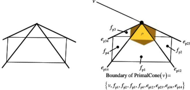
(3)

Every vertex v of a polytope  has an associated primal cone and dual cone.

In 3-dimension, the boundary of the primal cone PrimalCone v

 

consists of the vertex v , the facets

pi

f of  converging at the vertex v and the edges e converging at the vertex v so that an edge pij e pij

forms a common boundary between adjacent facets fpi and fpj (see fig. 3).

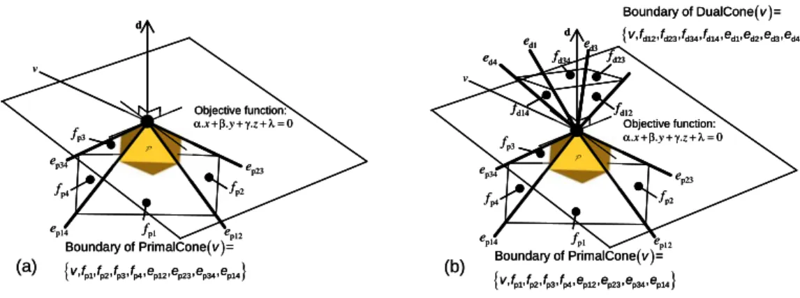
Let us consider an objective function of the shape: p x y z( , , )       .x .y .z and polytope  together define the function p x y z( , , ). The objective function is maximal on one face F (2-face, edge or vertex) of  . Let d be a normal to the objective function oriented towards the exterior of polytope  (see fig. 4a). The set of objective functions that reach their maximum in F is characterised by a polyhedral cone DualCone( )F defined by the set of normals d, thus in 3 [10]:







3



DualCone( )F :F : . max .       y d x d x d y    (4)

DualCone( )F is called the dual cone of polytope  in F. It is called the normal cone of polytope

 in F [10], [14]. The dual cone associated with a face of dimension i has a dimension



n i



in

n

(5)

p12 e p14 e p34 e p23 e p2 f p1 f p4 f p3 f d1 e e_d3 d4 e fd23 d12 f d34 f d14 f    d12 d23 d34 d14 d1 d2 d3 d4 Boundary of DualCone = , , , , , , , , v v f f f f e e e e v  d .x .y .z 0         Objective function:    p1 p2 p3 p4 p12 p23 p34 p14 Boundary of PrimalCone = , , , , , , , , v v f f f f e e e e p12 e p14 e p34 e p23 e p2 f p1 f p4 f p3 f v  d .x .y .z 0         Objective function:    p1 p2 p3 p4 p12 p23 p34 p14 Boundary of PrimalCone = , , , , , , , , v v f f f f e e e e (b) (a) p12 e p14 e p34 e p23 e p2 f p1 f p4 f p3 f d1 e e_d3 d4 e fd23 d12 f d34 f d14 f    d12 d23 d34 d14 d1 d2 d3 d4 Boundary of DualCone = , , , , , , , , v v f f f f e e e e v  d .x .y .z 0         Objective function:    p1 p2 p3 p4 p12 p23 p34 p14 Boundary of PrimalCone = , , , , , , , , v v f f f f e e e e p12 e p14 e p34 e p23 e p2 f p1 f p4 f p3 f v  d .x .y .z 0         Objective function:    p1 p2 p3 p4 p12 p23 p34 p14 Boundary of PrimalCone = , , , , , , , , v v f f f f e e e e p12 e p14 e p34 e p23 e p2 f p1 f p4 f p3 f d1 e e_d3 d4 e fd23 d12 f d34 f d14 f d1 e e_d3 d4 e fd23 d12 f d34 f d14 f    d12 d23 d34 d14 d1 d2 d3 d4 Boundary of DualCone = , , , , , , , , v v f f f f e e e e v  d .x .y .z 0         Objective function:    p1 p2 p3 p4 p12 p23 p34 p14 Boundary of PrimalCone = , , , , , , , , v v f f f f e e e e p12 e p14 e p34 e p23 e p2 f p1 f p4 f p3 f v  d .x .y .z 0         Objective function:    p1 p2 p3 p4 p12 p23 p34 p14 Boundary of PrimalCone = , , , , , , , , v v f f f f e e e e (b) (a)

Fig. 4 Definition of a dual cone - Dual cone and primal cone attached to a vertex.

Let us consider the dual cone of polytope  DualCone v

 

associated with the vertex v . In 3 this cone is 3-dimension given that the dimension of vertex v is 0. It consists of the vertex v , facets fdij that converge at v with their normals being respectively edges e and edges pij edi converging in v and these are in turn normal to facets fpi.

Fig. 4b shows the primal cone and the dual cone associated with the vertex v of polytope  .

2.3. Fan and normal fan

A fan in _n

is a family  



C1,....,Ck



of polyhedral cones with the following properties:

 each non-empty face of a cone in  is also a cone in ,

 the intersection of two cones in  is a face common to the two cones. The fan  is complete if and only if:

1 k n i i C     [10].

For any facet F of polytope  , the set of dual cones DualCone( )F partitions n. The set of dual cones defines a fan, which we will call the normal fan [9], [10].

The normal fan associated with polytope  is: N

 

 .

Let 1 and 2 be two fans of n

 . Then the common refinement of 1 and 2 [10] is:





1 2 C1 C2:C1 1,C2 2

         (5)

To determine the common refinement of two fans 1 and 2 a normal fan has to be determined

which consists of the set of all the intersections of the dual cones of the two fans 1 and 2 considered

two by two.

3. Minkowski sum by operations on dual cone

3.1. Problems in determining the Minkowski sum for two polytopes 3.1.1. Properties of dual cones

(6)



n| , :



   c  a  b c a b 

      (6)

In 1-dimension, this consists of adding together variables with boundaries at certain intervals.

For 2 and 3 dimensions, the Minkowski sum consists of carrying out a sweep from a reference point on one operand at the boundary of the other operand [11], [13].

In _2

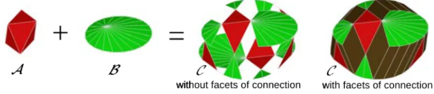
, the edges of the polytope sum are translations of the edges of the two operand polytopes [11], [13]. In 3, certain facets of the polytope sum are translations of the facets of the two operand polytopes. However, other facets are created, which we will call facets of connection. Thus it is not possible to deduce the facets of the polytope sum knowing only the facets of the operand polytopes. This property is illustrated in fig. 5 and discussed in [11], [13].

+

₌

  

without facets of connection with facets of connection



+

₌

  

without facets of connection with facets of connection



Fig. 5 Minkowski sum of 3 polytopes.

The work of [11], [13] can be further justified. The following property developed in [9], and also mentioned in [10] and [14], shows that the normal fan N

 

 of polytope  , the Minkowski sum of

polytopes  and  , is the common refinement of the two normal fans of polytopes  and  :

 



+



 

N  N   N  N  (7)

According to (5), determining the common refinement of two normal fans is based only on intersections of dual cones considered two by two. It is therefore not possible to create new edges in 2-dimension when determining the normal fan N

 

 . This is the reason why there is no facet of

connection in the Minkowski sum for two polytopes. In 3-dimension, new edges can be created. According to (4) and the properties of the dual cones cited in §2.2, these new edges are normals to the facets of connection of the polytope sum.

In this article we propose a method to construct facets of the polytope sum  based solely on intersections of dual cones on operands  and  .

We can then determine: the Minkowski vertices of  , the dual cones associated with the vertices of  and the normal fan N

 

 .

From the vertices of  and the respective dual cones, the facets of  can be defined.

Finally, using the proximity of the dual cones in the normal fan N

 

 , the ordered edges defining the

limits of the support hyperplane will be determined in order to define each facet of  .

3.2. Determining the vertices of the Minkowski sum of polytopes

Let the points of a face of polytope  maximising the objective function characterised by the vector be α :





S( , ) : . max .     y α x α x α y    (8)

(7)

Let us consider the following property:

Let a be a vertex of  and DualCone( )a the associated dual cone.

We have: DualCone

 

a S



,

  



  

α  α a (9)

Let  ,  and  be three polytopes such that:    . + =

Let a and b be two vertices of  and  respectively. Let us consider the following property:



a b



is a vertex of    γ 0: S(, )γ 

 

a et S(, )γ 

 

b (10)

This property expresses the fact that if the same objective function reaches its maximum at  in a single vertex a and at  in a single vertex b then



a b



is a vertex of  .

Any vertex of    is the sum of a vertex of  and a vertex of  according to Ewald's 1.5   theorem [15].

Using the previous properties, we can deduce eq. 11:



  



  



  

 

Let us consider and two vertices of and :

vertex of the Minkowski sum + such , and ,

o

such , DualCone dimension of DualCone

a b S a S b S c c c n               c = a + b γ 0 γ γ γ 0 γ γ         (11) + Polytope A Polytope B Polytope C = A + B = c a b _{DualCone a}_{ } _{DualCone b}_{ }     DualConeaDualConeb   PrimalCone a PrimalCone b  Scale1.5 + Polytope A Polytope B Polytope C = A + B = c a b _{DualCone a}_{ } _{DualCone b}_{ }     DualConeaDualConeb   PrimalCone a PrimalCone b  Scale1.5 + Polytope A Polytope B Polytope C = A + B = a b   DualCone a DualCone b  Scale1.5     DualConeaDualConeb + Polytope A Polytope B Polytope C = A + B = a b   DualCone a DualCone b  Scale1.5     DualConeaDualConeb (a) (b) + Polytope A Polytope B Polytope C = A + B = c a b _{DualCone a}_{ } _{DualCone b}_{ }     DualConeaDualConeb   PrimalCone a PrimalCone b  Scale1.5 + Polytope A Polytope B Polytope C = A + B = c a b _{DualCone a}_{ } _{DualCone b}_{ }     DualConeaDualConeb   PrimalCone a PrimalCone b  Scale1.5 + Polytope A Polytope B Polytope C = A + B = a b   DualCone a DualCone b  Scale1.5     DualConeaDualConeb + Polytope A Polytope B Polytope C = A + B = a b   DualCone a DualCone b  Scale1.5     DualConeaDualConeb + Polytope A Polytope B Polytope C = A + B = c a b _{DualCone a}_{ } _{DualCone b}_{ }     DualConeaDualConeb   PrimalCone a PrimalCone b  Scale1.5 + Polytope A Polytope B Polytope C = A + B = c a b _{DualCone a}_{ } _{DualCone b}_{ }     DualConeaDualConeb   PrimalCone a PrimalCone b  Scale1.5 + Polytope A Polytope B Polytope C = A + B = a b   DualCone a DualCone b  Scale1.5     DualConeaDualConeb + Polytope A Polytope B Polytope C = A + B = a b   DualCone a DualCone b  Scale1.5     DualConeaDualConeb (a) (b)

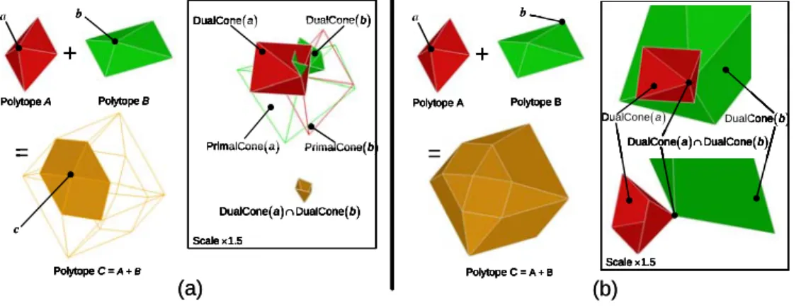
Fig. 6 Intersection of dual cones generating a vertex. Fig. 11 Intersection of dual cones not generating vertex.

Let us consider DualCone( )a and DualCone( )b the respective dual cones of polytopes  at vertex

a and  at vertex b .

If



DualCone( )a DualCone( )b



is 3-dimension, then



a b



c where c is the vertex of  : see

fig. 6a.

If





is clearly less than 3-dimension, then



a b



is not a vertex of  :

see fig. 6b.

There is a corollary which consists in determining the number of non-coplanar edges in

(8)

3.2.1. Proposal for an algorithm

From eq. 11, we are able to formulate an algorithm to determine the vertices of the Minkowski sum. In addition, determining





for all the vertices of  and  gives the common refinement of  and  according to eq. 5 and hence we can deduce the normal fan N 

 

.

Require: two 3-polytopes  and 

Ensure: determination of Lv C, , LDualCone,C and N  with  + =

1: k 0

2: for each vertex aiofA with Lf A, do DualCone a i

4: for each vertex bjofB with Lf B, do DualCone bj ; compute Iij= DualCone ai DualCone bj

5: if dimension of Iij then 3 k  ; compute k 1 ck ai b ; add j c in k Lv C, ; add Iij=DualCone ck in LDualCone,C

6: end if

7: end for

8: end for

9: nv C,  ; k N  DualCone ckwith DualCone ck LDualCone,C

Fig. 7 Determining the vertices of the Minkowski sum of 3-polytopes.

Polytope  is characterised by its list of vertices Lv A, and its list of facets Lf A, .

Let ai be the i

th

vertex of Lv A, . We have: 1 i nv A, where nv A, is the number of vertices of  .

In the same way, polytope  is characterised by Lv B, and Lf B, .

Let bj be the j

th

vertex of Lv B, . We have: 1 j nv B, where nv B, is the number of vertices of  .

Polytope  is characterised by its list of vertices Lv C, , its list of dual cones LDualCone,C and its normal fan

 

N  .

Let ck be the k

th

vertex of Lv C, . We have: 1 k nv C, where nv C, is the number of vertices of  .

Let DualCone

 

c_k be the kth dual cone of  associated with ck of LDualCone,C.

The fig. 7 presents the algorithm to determine the vertices of the Minkowski sum of 3-polytopes.

3.3. Determining the facets of the Minkowski sum of polytopes 3.3.1. Properties of dual cones

We shall go straight to eq. 4 developed in [10].

3

Property 1: In , dual cones associated with vertices of the same facet of a polytope share one and the same edge in the polytope's normal fan.

i

k v



(12)

Fig. 8a shows the 4 dual cones DualCone

 

ck associated respectively with vertices c c c1, 2, 3andc on 4

the same facet f of polytope  . The 4 dual cones DualCone

 

c_k are translated on vertex c1. They

(9)

 

DualCone c_k associated respectively with vertices ck (where 1  ) is normal to facet k 4 f : see

fig. 8a.

Property 2: the two dual cones associated with the two vertices of the same edge of a polytope

share a single face in the polytope's normal fan (13)

Fig. 8a illustrates property 2 for the edge of polytope  bounded by vertices c1 and c2.

3.3.2. Proposal for an algorithm

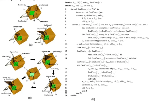
Fig. 8 Determining the facets of the Minkowski sum of 3-polytopes.

From the two properties described earlier, an algorithm can be formulated to search for the facet edges of a 3 polytope when its vertices, its normal fan and the dual cones associated respectively with the polytope vertices are known. From property 1 (12) in the normal fan of a polytope, the edge common to the dual cones associated with the primal vertices of the same facet can be identified. From property 2 (13), we can turn around this common edge and identify the vertices of this facet in order.

Polytope  is characterised by its list of vertices Lv C, , its list of dual cones LDualCone,C and its normal fan

 

N  . Let ck be the k

th

vertex of Lv C, . We have: 1 k nv C, where nv C, is the number of vertices of  .

Let DualCone

 

ck be the k th

dual cone  associated with ck of LDualCone,C.

c1 c4 c3 c2 DualCone(c2) DualCone(c3) DualCone(c4) DualCone(c1) Cl f c1 Common edge Cl f c1 c4 Common face DualCone(c4) DualCone(c1) Cl f c1 c4 c3 c2 DualCone(c2) DualCone(c3) DualCone(c4) DualCone(c1) Cl f c1 c4 c3 c2 DualCone(c2) DualCone(c3) DualCone(c4) DualCone(c1) Cl f c1 Common edge Cl f c1 Common edge Cl f c1 c4 Common face DualCone(c4) DualCone(c1) Cl f c1 c4 Common face DualCone(c4) DualCone(c1) Cl f cl f

Common face DualCone(c2)

DualCone(c3) c4 c3 c2 cl f c1 cl f c1 c2 DualCone(c1) DualCone(c2) Common face cl f DualCone(c4) c1 DualCone(c1) Common face c4 cl f DualCone(c3) c4 c3 DualCone(c4) Common face c3 c2 cl f

Common face DualCone(c2)

DualCone(c3) c4 c3 c2 cl f c1 cl f c1 c2 DualCone(c1) DualCone(c2) Common face cl f DualCone(c4) c1 DualCone(c1) Common face c4 cl f DualCone(c3) c4 c3 DualCone(c4) Common face c3 c2 (a) (c) _(b)

Require: Lv C,, N  and nv C, DualCone ck

Ensure: Lf C, and Le f,Cl for each f Cl

1: for each DualCone ck ofN( ) do 2: for each e of du DualCone ck do

3: compute h defined by Cl c and k e du 4: if h is not in Cl Lh C, then 5: add h in Cl Lh C,

6: find the qDualCone cm in N  such that: eduDualCone cm DualCone ck with m . k

7: find DualCone cm1 among the q DualCone cm such that:

 1   1

DualConecm DualConeck fdv, facet of DualCone ck

8: find DualCone cm2 among the q DualCone cm such that:

 2   2

DualConecm DualConeck fdv, facet of DualCone ck with fdv1fdv2 9: h is the support hyperplane of Cl f and Cl ne f,cl  . q 1

10: c and k c limit the first edge m1 efCl1 of f , add Cl efCl1 in Le f,Cl

11: DualCone cmp= DualCone cm1 12: DualConecmp1= DualCone ck

13: while DualCone cmp DualCone cm2 do

14: find DualConecmp1 among the q DualCone cm such that:  1  

DualConecmp DualConecmpfdmp, facet of DualCone cmp

with DualConecmp1DualConecmp1

15: cmp and cmp1 limit the next edge efClw of f , add Cl efClw in Le f,Cl

16 : DualConecmp1DualCone cmp

17: DualCone cmp DualConecmp1 18: end while

19: cmpcm2 and c limit the last edge k efClq of f , add Cl efClw in Le f,Cl

20: determine f with Cl h and Cl Le f,Cl

21: add f in Cl Lf C, 22: end if

23: end for

(10)

We postulate DualCone

  

ck  c ek, du,fdv



where: du

e is the uth edge of DualCone

 

ck and fdv is the v th

facet of DualCone

 

ck .

Let Lf C, be the list of facets of  .

We represent as fCl the l

th

facet of Lf C, (1 l nf C, where nf C, is the number of facets of  ).

Let Lh C, be the list of support hyperplanes for  .

Let hCl be the l

th

hyperplane of Lh C, (1 l nf C, )

Let Le f, Cl be the ordered list of the edges of facet fCl. Two consecutive edges of Le f, Cl share a single

vertex and the first and last edges. Let

Clw

f

e be the wth edge of fCl.(1 w ne f,cl where ne f,cl is the number of edges of fCl).

The fig. 8b presents the algorithm to determine the facets of the Minkowski sum of 3-polytopes.

Fig. 8c shows stages 7 to 18 of the algorithm for determining the edges of a facet fcl of polytope  of vertices c c c1, 2, 3andc4. It corresponds to a case where: k 1 ck c1andq 3 ne f,cl  . 4

To be more precise, fig. 8c shows the determination of the first edge, bounded by c1andc2 and vertex 4

c , the last vertex in the outline of fcl where: m12 andm24.

It shows the determinations of the edges bounded by:  c₂andc₃ where mp 2 andmp1 , 3

 c₃andc₄ where mp 3 andmp1 , 4

 c₄andc₁ where mpm24 andk . 1

4. Discussion of the proposed method

The determination method proposed in this article is based solely on intersections of pairs of dual cones associated with searches for common edges and faces of dual cones in a normal fan.

Using this algorithm, nv A, nv B, intersections of pairs of dual cones have to be calculated in order to

determine the vertices of polytope  and the normal fan N 

 

.

In addition, it is necessary to carry out nf c, searches for a common edge among the dual cones in the

normal fan N

 

 . Finally, , , 1 f c cl Cl n e f Cl n  



searches are needed for a common face between dual cones to determine the edges of polytope  . Each search for a common face is carried out in a sub-set of dual cones in the normal fan N

 

 which share an edge.

Each vertex of polytope  is the sum of two vectors associated respectively with two vertices of polytopes  and  . From the nv A, nv B, intersections of pairs of dual cones it is possible to determine

from which vertices of operands  and  the vertices of  derived.

In addition, the normal for each facet of  is characterised by an edge in the normal fan N

 

 . Thus

the translated facets can be differentiated from the facets of connection.

Each normal of the facets of connection is generated by the intersection of two dual cones and more precisely by the intersection of two faces of dual cones. In this way, we can identify the facets of operands  and  from which the normals of the facets of connection derive.

(11)

The normals of facets that are different from the facets of connection derive either from operand  , or operand  . The method proposed here gives complete traceability of the vertices and facets of polytope  from the vertices and facets of operands  and  . In tolerance analysis, this traceability is used to optimise the filling of a functional polytope by a calculated polytope.

The proofs of properties (11), (12) and (13) are detailed in [16].

These algorithms are currently being developed in the topological structure of an OpenCASCADE distribution [17].

The intersection algorithm used in this work is the OpenCASCADE 6.2 distribution algorithm.

5. Conclusion and future research

We have shown how to determine the Minkowski sum for two 3 polytopes from intersections of polyhedral cones and using the properties of the common edge and common face between dual cones in a normal fan. The algorithms for determining the vertices and the facets have been described. Ultimately, this method will be applied in a tolerance analysis procedure in an environment that can be multi-physical [6]. Work is currently underway on a method to determine the intersection of two polyhedral cones so that this can be generalised for n dimension polytopes. It will allow to transpose the algorithms of this

article in a n dimension according to the property computing common refinement (7). This work will be described in a later publication.

References

[1] G. Elber, M.S. Kim, Offsets, sweeps, and Minkowski sums, Computer-Aided Design. 31 (1999) 163. [2] A. Fleming, Geometric relationships between toleranced features, Artificial Intelligence. 37 (1988) 403-412.

[3] M. Giordano, D. Duret, Clearance Space and Deviation Space, dans: Proc. of 3rd CIRP seminar on Computer Aided Tolerancing, ISBN 2-212-08779-9, Cachan (France), 1993: p. 179-196.

[4] U. Roy, B. Li, Representation and interpretation of geometric tolerances for polyhedral objects. II.: Size, orientation and position tolerances, Computer-Aided Design. 31 (1999) 273-285.

[5] J.K. Davidson, A. Mujezinovic, J.J. Shah, A new mathematical model for geometric tolerances as applied to round faces, ASME Transactions on Journal of Mechanical Design. 124 (2002) 609-622.

[6] L. Pierre, D. Teissandier, J.P. Nadeau, Integration of thermomechanical strains into tolerancing analysis, International Journal on Interactive Design and Manufacturing. 3 (2009) 247-263.

[7] A.A.G. Requicha, Toward a theory of geometric tolerancing, The International Journal of Robotics Research. 2 (1993) 45-60.

[8] D. Teissandier, V. Delos, Operations on polytopes: application to tolerance analysis, dans: Proc. of 6th CIRP Seminar on Computer Aided Tolerancing, ISBN 0-7923-5654-3, Enschede (Netherlands), 1999: p. 425-433.

[9] P. Gritzmann, B. Sturmfels, Minkowski addition of polytopes: computational complexity and applications to Gröbner bases, Siam Journal of Discrete Mathematics. 6 (1993) 246-269.

[10] G. Ziegler, Lectures on polytopes, ISBN 0-387-94365-X, Springer Verlag, 1995.

[11] Y. Wu, J.J. Shah, J.K. Davidson, Improvements to algorithms for computing the Minkowski sum of 3-polytopes, Computer-Aided Design. 35 (2003) 1181-1192.

[12] P.K. Ghosh, A unified computational framework for Minkowski operations, Computers & Graphics. 17 (1993) 357-378. [13] H. Barki, F. Denis, F. Dupont, Contributing vertices-based Minkowski sum computation of convex polyhedra,

Computer-Aided Design. 41 (2009) 525-538.

[14] K. Fukuda, From the zonotope construction to the Minkowski addition of convex polytopes, Journal of Symbolic Computation. 38 (2004) 1261-1272.

[15] G. Ewald, Combinatorial Convexity and Algebraic Geometry, ISBN 9780387947556, Springer, 1996.

[16] D. Teissandier, V. Delos, Algorithm to calculate the Minkowski sums of 3-polytopes based on normal fans, Computer-Aided Design. 43 (2011) 1567-1576.