Uncertainty in projected climate change arising from uncertain fossil-fuel emission factors

HAL Id: hal-01806850

https://hal.archives-ouvertes.fr/hal-01806850

Submitted on 16 Sep 2020

HAL is a multi-disciplinary open access

archive for the deposit and dissemination of

sci-entific research documents, whether they are

pub-lished or not. The documents may come from

teaching and research institutions in France or

abroad, or from public or private research centers.

L’archive ouverte pluridisciplinaire HAL, est

destinée au dépôt et à la diffusion de documents

scientifiques de niveau recherche, publiés ou non,

émanant des établissements d’enseignement et de

recherche français ou étrangers, des laboratoires

publics ou privés.

Distributed under a Creative Commons Attribution| 4.0 International License

Uncertainty in projected climate change arising from

uncertain fossil-fuel emission factors

Y Quilcaille, G Gasser, P. Ciais, F. Lecocq, G. Janssens-Maenhout, S. Mohr

To cite this version:

Y Quilcaille, G Gasser, P. Ciais, F. Lecocq, G. Janssens-Maenhout, et al.. Uncertainty in projected

climate change arising from uncertain fossil-fuel emission factors. Environmental Research Letters,

IOP Publishing, 2018, 13 (4), �10.1088/1748-9326/aab304�. �hal-01806850�

LETTER • OPEN ACCESS

Uncertainty in projected climate change arising

from uncertain fossil-fuel emission factors

To cite this article: Y Quilcaille et al 2018 Environ. Res. Lett. 13 044017

View the article online for updates and enhancements.

Related content

Are the impacts of land use on warming underestimated in climate policy?

Natalie M Mahowald, Daniel S Ward, Scott C Doney et al.

-Contributions of developed and developing countries to global climate forcing and surface temperature change

D S Ward and N M Mahowald

-The impact of aerosol emissions on the 1.5 °C pathways

Anca Hienola, Antti-Ilari Partanen, Joni-Pekka Pietikäinen et al.

-Recent citations

The contribution of carbon dioxide emissions from the aviation sector to future climate change

E Terrenoire et al

Environ. Res. Lett. 13 (2018) 044017 https://doi.org/10.1088/1748-9326/aab304

LETTER

Uncertainty in projected climate change arising from

uncertain fossil-fuel emission factors

Y Quilcaille1,2,6 _{, T Gasser}3_{, P Ciais}1_{, F Lecocq}2_{, G Janssens-Maenhout}4_{and S Mohr}5

1 _{Laboratoire des Sciences du Climat et de l’Environnement, LSCE/IPSL, Universit´e Paris Saclay, CEA—CNRS—UVSQ, 91191}

Gif-sur-Yvette, France

2 _{Centre International de Recherche sur l’Environnement et le D´eveloppement (CIRED),}

CNRS—PontsParisTech—EHESS—AgroParisTech—CIRAD, 94736 Nogent-sur-Marne, France

3 _{International Institute for Applied Systems Analysis (IIASA), 2361 Laxenburg, Austria} 4 _{European Commission, Joint Research Centre, 21027 Ispra, Italy}

5 _{Institute for Sustainable Futures, University of Technology Sydney, UTS Building 10, 235 Jones St., Ultimo, NSW 2007, Australia} 6 _{Author to whom any correspondence should be addressed.}

OPEN ACCESS

RECEIVED 27 October 2017 REVISED 2 February 2018 ACCEPTED FOR PUBLICATION 1 March 2018 PUBLISHED 29 March 2018

Original content from this work may be used under the terms of the Creative Commons Attribution 3.0 licence. Any further distribution of this work must maintain attribution to the author(s) and the title of the work, journal citation and DOI.

E-mail:quilcail@centre-cired.fr

Keywords: emissions, climate, fossil fuels, uncertainty, Earth system modelling Supplementary material for this article is availableonline

Abstract

Emission inventories are widely used by the climate community, but their uncertainties are rarely

accounted for. In this study, we evaluate the uncertainty in projected climate change induced by

uncertainties in fossil-fuel emissions, accounting for non-CO

species co-emitted with the

combustion of fossil-fuels and their use in industrial processes. Using consistent historical

reconstructions and three contrasted future projections of fossil-fuel extraction from Mohr et al we

calculate CO

emissions and their uncertainties stemming from estimates of fuel carbon content, net

calorific value and oxidation fraction. Our historical reconstructions of fossil-fuel CO

emissions are

consistent with other inventories in terms of average and range. The uncertainties sum up to a ±15%

relative uncertainty in cumulative CO

emissions by 2300. Uncertainties in the emissions of non-CO

species associated with the use of fossil fuels are estimated using co-emission ratios varying with time.

Using these inputs, we use the compact Earth system model OSCAR v2.2 and a Monte Carlo setup, in

order to attribute the uncertainty in projected global surface temperature change (ΔT) to three

sources of uncertainty, namely on the Earth system’s response, on fossil-fuel CO

emission and on

non-CO

co-emissions. Under the three future fuel extraction scenarios, we simulate the median ΔT

to be 1.9, 2.7 or 4.0

C in 2300, with an associated 90% confidence interval of about 65%, 52% and

42%. We show that virtually all of the total uncertainty is attributable to the uncertainty in the future

Earth system’s response to the anthropogenic perturbation. We conclude that the uncertainty in

emission estimates can be neglected for global temperature projections in the face of the large

uncertainty in the Earth system response to the forcing of emissions. We show that this result does not

hold for all variables of the climate system, such as the atmospheric partial pressure of CO

and the

radiative forcing of tropospheric ozone, that have an emissions-induced uncertainty representing

more than 40% of the uncertainty in the Earth system’s response.

1. Introduction

Sources of uncertainty in climate change projections are numerous (Cox and Stephenson 2007, Hawkins and Sutton 2009, Allen et al 2000), ranging from the future evolution of anthropogenic drivers of cli-mate change like future greenhouse gas and aerosol

emissions, to the modeling of the Earth system’s response. Scenarios based on contrasted socio-economic storylines and an ensemble of integrated assessment models (Moss et al 2010, O’Neill et al

2014) are used to explore the uncertainty in future human activities. For such a given emission scenario, the uncertainty in climate change is estimated by using

different Earth system models (Flato et al 2013) to translate emissions into changes in concentrations, radiative forcing and climate. However, the extent in which the uncertainty in emissions affects climate change projections is not well known.

Fossil fuel use is the largest anthropogenic driver of the climate system. The burning of fossil fuels emits carbon dioxide (CO₂) to the atmosphere, and the fraction of CO2 remaining airborne is the largest

anthropogenic forcing of climate change. Other cli-mate forcing agents such as carbon monoxide (CO), sulfur dioxide (SO2) or nitrogen oxides (NOx) are

also co-emitted with the burning of fossil fuels, their use as feedstock in various industrial processes. During their extraction, fugitive emissions occur,in particular methane (CH₄) (Kirschke et al2013, EEA2013). The amount of each species emitted by these three activities related to fossil fuels is estimated via emission inven-tories, which combine activity data such as the mass of fuel used or the energy obtained from these fuels, with emission factors related to the carbon content of fuels and to technologies that produces co-emitted species (EEA2013).

Because of the various methodologies and input data they use, different emission inventories show dif-ferences in their estimates of fossil CO₂ emissions (e.g. Olivier2002, Marland et al2009, Andres et al

2012). At a national scale, the major sources of uncer-tainties in inventories may be emission factors (Zhao

et al2011), although this remains unsure at a global scale. The 2006 IPCC Guidelines for National GHG

Inventories (IPCC2006) recommend to use a mean carbon content for lignite of 101 kgCO₂/GJ with a range from 91 to 115 kgCO2/GJ (95% confidence

interval); hence a 10% uncertainty in the CO₂ emis-sions from lignite. For co-emitted non-CO₂ species, the uncertainty is much larger because their emissions depend not only on the composition of each fuel (in carbon, sulfur, nitrogen) but also on technologies that determine the fuel-use efficiency in different sectors, on the presence, enforcement of use, and efficiency of emission control devices (e.g. stack desulfurization) and on operating conditions (EEA2013, IPCC2006, Granier et al 2011). For instance, according to the

EMEP/EEA Air Pollutant Emission Inventory Guide-book 2013 (EEA2013), the emission factor of CO for the burning of brown coal to produce electricity and heat is 8.7 gCO/GJ, but the associated 95% confidence interval ranges from 6.7 to 60.5 gCO/GJ. This means that a given amount of energy produced by the com-bustion of brown coal comes with a −20 to +600% uncertainty on CO emissions. Albeit CO has a minor contribution on climate change compared to other compounds such as CO₂, its impact on air quality is stronger (Crippa et al2016).

In this study, we investigate how uncertainty in emission factors for CO₂ and non-CO₂ emissions associated with the combustion of fossil-fuels and their use in industrial processes affects climate change

projections. First, we calculate ranges of uncertainty in CO₂and non-CO₂fossil-fuel co-emissions for histor-ical and for three contrasted future scenarios of fossil fuel extraction. Second, we translate this uncertainty into a range of radiative forcing and climate change using the OSCAR v2.2 Earth system model, using a Monte-Carlo approach. Finally, we analyze the vari-ance of the system and compare the uncertainty from emission factors to the one on the temperature response to emissions through Earth system processes.

2. Methods

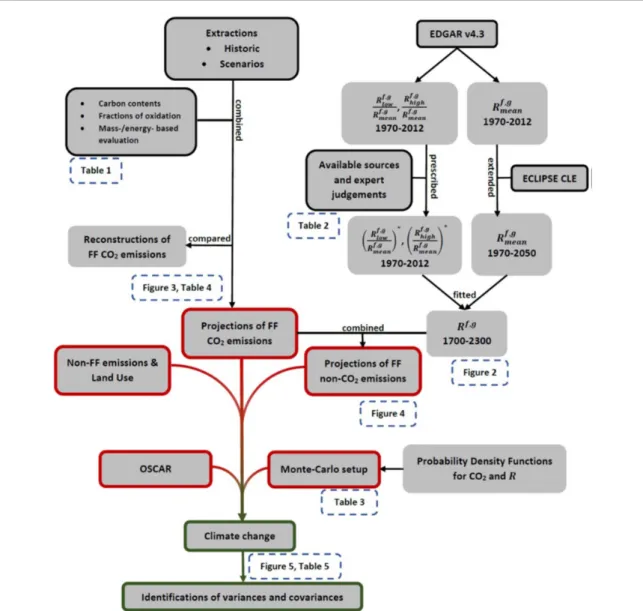
An overview of our method is described in figure1. Extraction scenarios (section2.1) are combined with carbon contents, net calorific values and fractions of oxidations (section2.2) to produce fossil-fuel CO₂ pro-jections. To evaluate the fossil-fuel co-emissions, we calculate co-emission ratios, which are factors linking the fossil-fuel CO₂emissions to the non-CO₂emissions associated with fossil fuels (section 2.3). We com-plete these projections with non-fossil-fuel emissions and other anthropogenic drivers (section2.4). Finally, the reduced-form Earth system model OSCAR is used with these drivers through a Monte-Carlo setup (sec-tion2.5) to evaluate all required uncertainties. 5% and 95% quantiles are calculated to obtain the confidence intervals, whereas variances are used to calculate each contribution to the total variance.

2.1. Extraction scenarios

We take the historical reconstruction of fossil-fuel extraction (1750–2012) and three future extraction scenarios (up to 2300) made by Mohr et al (2015). Country-scale data is aggregated to the global scale for eight types of coal, five types of oil and five types of gas. Peat extraction, flaring and cement production are not included. The three future extraction scenarios were produced with the GeRS-DeMo model (Mohr and Evans2010). Additionally, since conversion factors are provided by Mohr et al (2015), historical reconstruction and scenarios can be expressed both in energy values and in mass of extracted fuels. The future abundance in fossil fuels remains uncertain (Ward et al (2012), but this uncertainty is not included here. We use only three future scenarios, differing by their assumptions regard-ing ultimately recoverable resources, with a ‘Low’, ‘Best Guess’ (called ‘Medium’ hereafter) and ‘High’ case. For comparison, the Low scenario is between RCP2.6 and RCP4.5, the Medium close to RCP4.5 and the High near to RCP6.0 (Van Vuuren et al2011). These scenarios include no climate policy or transition to non-fossil energy sources (unlike RCPs Clarke et al

2014) or SSPs (Riahi et al2017), but this is not a lim-itation for our study since we focus on the climate change uncertainty induced by uncertain emission fac-tors and for this purpose, we just need fossil-fuel scenarios comparable to those showed by the IPCC.

Environ. Res. Lett. 13 (2018) 044017

Figure 1. Overview of the method used in this study. For different parts, we give references to the relevant tables and figures. ‘FF’ stands here for fossil-fuel, and R corresponds to co-emission ratios.

The Mohr et al scenarios have the advantage of docu-menting fuel extraction of various fuel types (allowing us to address uncertainty on carbon contents) and to be fully consistent regarding the different fuel types between the historical and future periods.

2.2. CO2emissions

When calculated from energy-based fuel extraction data (superscriptene), CO₂ emissions in kgC yr−1 resulting from the use of a type f fuel are given by:

𝐸CO2

𝑓 = 𝐹 𝑂𝑓𝐶𝑓𝑒ene𝑓 (1)

where C_𝑓 is the fuel carbon content in kgC J−1 pro-duced, FO_𝑓 the fraction oxidized of the extracted fuel (unitless) through combustions and uses, and

𝑒ene

𝑓 the amount of fuel extracted in J yr−1. When

calculated from mass-based fuel extraction data (superscriptphy),𝑒ene_𝑓 is adapted using NCV_𝑓, the net calorific value of the fuel in J per unit mass of extracted

fuel, and𝑒phy_𝑓 is the mass extracted per year:

𝐸CO2

𝑓 = 𝐹 𝑂𝑓𝐶𝑓NCV𝑓𝑒phy𝑓 (2)

To account for uncertain carbon contents or uncer-tain net calorific values—depending whether equation (1) or (2) is used—we use four different data sources to obtain six different values: Mohr et al (2015), CDIAC (Boden et al 1995, IPCC 1996), the IPCC (2006) average, and its lower and upper bounds of the 95% confidence interval (detailed values in appendix 1 available atstacks.iop.org/ERL/13/044017/ mmedia). The use of equation (1) or (2) is moti-vated by the differences observed in the sets of NCV and the associated uncertainties. The resulting different emission factors cause these two approaches not to be equivalent.

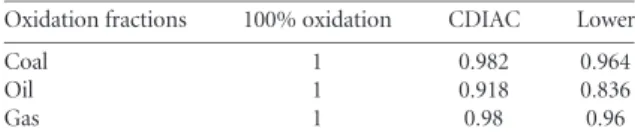
Regarding the uncertainty on oxidation fractions, we use the CDIAC values (Marland and Rotty1984) to produce three sets of oxidation fractions as shown in table1. These values are also applied globally. Note that we do not use the oxidation fractions from other 3

Table 1. Sets of oxidation fractions used. The lower case is built to be symmetrical to the 100% oxidation case with respect to the central CDIAC values (Marland and Rotty (1984)).

Oxidation fractions 100% oxidation CDIAC Lower

Coal 1 0.982 0.964

Oil 1 0.918 0.836

Gas 1 0.98 0.96

data sources, either because they are not explicitly reported, or because they are based on a different defini-tion. Here, the oxidation fraction defined as the fraction of the fuel oxidized during combustion in energy uses and during non-energy uses (Marland and Rotty

1984). We do not use the confidence intervals from (Marland and Rotty1984) because the Tier 1 default oxidation fractions of IPCC (2006) lies out of this inter-val, they are all equal 100%. However, the intervals that we define at a global scale may still be underestimated, Liu et al (2015) shows for the case of China a 92% oxidation rate.

The combination of the four carbon contents (one being a distribution), three oxidation fractions and two sources of fuel extraction data (energy-based or mass-based) provides us with a distribution of fossil-fuel CO₂ emission over the historical period and for each of the three future extraction scenarios.

2.3. Non-CO₂co-emissions associated with the use of fossil fuels

Non-CO2 species are co-emitted with CO2 during

fossil-fuel combustion and use in industrial processes because of non-carbon elements oxidized (e.g. sulfur giving SO2), high temperature combustions oxidizing

atmospheric nitrogen (N₂O and NO_X), or incom-plete combustion processes (CH₄, CO, BC, OC and VOCs). We also consider ammonia (NH₃) emissions which occur through leaks during the production of coke where ammonia is used to reduce nitrogen oxides (NOX) emissions (EEA 2013). Methane (CH4)

pro-duced during extraction, venting and flaring is however excluded. These species impact the climate system as greenhouse gases (CO2, CH4, N2O), ozone

precur-sors (CO, NO_X, VOCs), aerosols or aerosol precursors (SO₂, NH₃, NO_X, OC, and BC).

In order to link the emissions of co-emitted species with those of CO₂, we define co-emission ratios (R𝑓,𝑔) for each fuel f, and species g:

𝐸𝑓,𝑔 _{= 𝑅}𝑓,𝑔_𝐸𝑓,CO2 ₍₃₎

where E𝑓,𝑔 is the co-emission of g for the fuel f. Since we derive CO₂emissions from extraction and not consumption data (Davis et al2011), we have to use global and not regional co-emission ratios because we do not know where and though which technol-ogy each fuel is used. We evaluate global mean ratios (𝑅𝑓,𝑔_mean) for each co-emitted compound and for coal, oil and gas, using the EDGARv4.3.2 database (Olivier

et al2015) over 1970–2012 The matching of fuels is described in figure 2.1 of the appendix. These ratios

are extended to 2050 using the Current Legislation (CLE) scenario of ECLIPSEv5.0 (Stohl et al 2015). This scenario is consistent with the absence of climate policies in our extraction scenarios (Mohr et al2015). To back-cast these global ratios over the whole period (1750–2300), two different rules are created. The first rule is a constant extension of the average of the ratios over 1970–1975 to 1700–1970; and of that over 2007– 2012 to 2012–2300 (Constant rule). For the second rule we fit an S-shaped function over the 1970–2012 data from EDGARv4.3.2 and using the evolution to 2050 from ECLIPSEv5.0 as an additional constraint (Sigmoid rule). These two rules are shown in figure2.

To estimate the uncertainty in the co-emission ratios, we use an approach combining different elements. Relative uncertainty in global non-CO₂ emis-sion is taken from the literature whenever possible, and we made assumptions for the remaining species for which we did not find literature data, as shown in table2. We assume that the relative uncertainty in co-emission ratios is correlated to the inter-country spread in national co-emission ratios, weighted by national CO₂emissions. Under this assumption, if the weighted spread in national co-emission ratios for a specie increases two-fold over a period, the uncertainty in the global co-emission ratios increases two-fold as well. The weighting by emissions is used to give less importance to countries that have less industrial activity. To do so, we extract from EDGARv4.3.2 the co-emission ratios for 113 world regions (most of them being individual countries) (Narayanan and Walms-ley (2008)), we weight each region’s ratios by its CO₂ emissions, and we extract the resulting mean, 2.5th and 97.5th percentiles to define𝑅𝑓,𝑔mean,𝑅𝑓,𝑔_lowand𝑅𝑓,𝑔_high, the

difference𝑅𝑓,𝑔_highminus𝑅𝑓,𝑔_lowover 1970–2012 being the spread in weighted co-emission ratios. We then rescale

𝑅𝑓,𝑔_low∕𝑅𝑓,𝑔meanand𝑅𝑓,𝑔_high∕𝑅𝑓,𝑔meanusing the values and the

period of time or year shown in table2. Finally, we apply the Constant or Sigmoid extension rules as for𝑅𝑓,𝑔_mean to obtain the future uncertainties in the co-emission ratio of each species.

2.4 Non fossil-fuel emissions and other drivers

Past and future emissions from other sources than fossil-fuel (hereafter ‘background’ emissions) are pre-scribed as follows. For the historical period, we take CO₂ emissions caused by cement production and flaring from CDIAC (Boden et al 2013), and for other species we take existing inventories (EDGAR 4.2 JRC2011) and ACCMIP (Lamarque et al 2010) of which we remove the fossil-fuel related sectors. For 2011–2100, we take emissions from the non-fossil-fuel sectors of the RCP6.0 (Meinshausen et al2011). After 2100, we assume constant emissions at their levels of 2100. Note that the sectors associated with fossil-fuels in ACCMIP/RCP are slightly different from the sectors that we use. For instance, energy sector in ACCMIP/RCP include both fossil-fuels energies and

Environ. Res. Lett. 13 (2018) 044017

Figure 2. Co-emission ratios for SO2emitted when using coal (a), oil (b) and gas (c). The central black dotted line shows the global

ratio taken from the EDGAR v4.3.2 dataset (Olivier et al (2015)). The histogram of co-emission ratios for GTAP regions (Narayanan and Walmsley (2008)) is represented, with its confidence intervals (shaded areas). Colored lines show the two extrapolation: Sigmoid (pink) and Constant (green).

Table 2. Relative uncertainty and period of time or date of rescaling used for co-emission ratios.

Compound Relative uncertainty Year(s) of application Source SO2 ±12% 2000–2010 Smith et al2011[27] BC −32% to +118% 1996 Bond et al2004[28] OC −42% to +97% 1996 Bond et al2004[28] NOx ±30% 2003–2013 Janssens-Maenhout et al2015[29] CO ±20% 2003–2013 Janssens-Maenhout et al2015[29] CH4 ±10% 1990–2010 IPCC2006[12] N2O ±10% 1990–2010 IPCC2006[12]

VOC ±20% 2003–2013 Assumed same as CO

NH3 ±10% 1990–2010 Assumed same as N2O

biomass energies, whereas we excluded the latter in our analysis. Because of these discrepancies, the non-fossil fuels emissions of these datasets added to our fossil-fuel emissions sum up to a slightly different total of the ones of the inventories. However, this inconsistency has no impact on our results, since we focus on the uncertainty caused by emissions from fossil-fuel alone. Land-use and land-cover change data come from the LUH1.1 dataset (Hurtt et al2011) for 1750–2100. After 2100, land-cover is assumed constant, while har-vest and shifting cultivations keep their 2100 levels.

2.5. Climate change projections

We use the compact Earth system model OSCAR v2.2 (Gasser et al 2017a, Arneth et al 2017, Gasser

et al2017b) to simulate climate change given uncer-tain fossil-fuel emissions and co-emissions. This model includes all the relevant components of the Earth sys-tem: the oceanic and terrestrial carbon cycles, the tropospheric and stratospheric chemistries of non-CO₂ greenhouse gases and ozone, and the direct and indi-rect climate effects of aerosols (Gasser et al 2017a).

For each Earth system process it features, OSCAR v2.2 is calibrated on more complex models to emulate their own range of sensitivity.

To estimate the uncertainty in projected climate change, a probabilistic Monte Carlo framework is used. The Monte Carlo ensemble is made of 1000 ele-ments drawn by taking randomly: Earth system-related parameters (66 parameters of OSCAR v2.2, see table

3of Gasser et al 2017a); the method through which fossil-fuel CO2emissions are calculated, energy-based

or mass-based extractions (two options), carbon con-tents or net calorific values (four options since here we use the IPCC-2006 data [12] as a distribution), oxi-dation fractions (three options); and non-CO₂species co-emission ratios (27 distributions from since we have nine species times three fuels).

When we have several distinct options, e.g. for the parameters of OSCAR or the choice of energy-based or mass-energy-based fuel extraction data, each option is given the same probability. For variables related to CO₂emissions and co-emission ratios, we fit a distri-bution over these probabilities and then draw a random 5

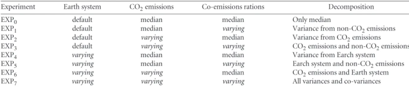
Table 3. Categories of simulations to attribute the uncertainty in projected climate change to Earth system response, CO2emissions and

non-CO2species co-emissions. For each element of the Monte Carlo ensemble, the eight simulations of each line of the table are generated

and used for the attribution to the variances and covariances.

Experiment Earth system CO2emissions Co-emissions rations Decomposition

EXP0 default median median Only median

EXP1 default median varying Variance from non-CO2emissions

EXP2 default varying median Variance from CO2emissions

EXP3 default varying varying CO2emissions and non-CO2emissions

EXP4 varying median median Variance from Earch system

EXP5 varying median varying Earch system and non-CO2emissions

EXP6 varying varying median CO2emissions and Earth system

EXP7 varying varying varying All variances and co-variances

value from this distribution. According to IPCC (2006), we use lognormal distributions for CO₂ emissions, whereas lognormal or gamma distributions are used for co-emission ratios, depending on the quality of the fit. We assume the same drawn point in the distribution for all years, therefore we assume a 100% correlation of the uncertainty through time.

For each element of the ensemble, we produce eight categories of simulations with OSCAR v2.2 in which the Earth system parameters, the parameters of fossil-fuel CO₂emissions, and those of co-emitted species emis-sions are either the drawn value or kept constant (see table3). The results of these simulations are used to analyze the uncertainty in projected climate change by attributing the variance of global temperature change to each one of the three sources of uncertainty, on the Earth system response, on CO2emissions, and on

non-CO₂co-emissions (their ratios to CO₂emissions). We point out however that the default configuration of OSCAR is used as a proxy of what would be a hypothet-ical (non-existing) ‘median’ configuration. The small difference between these two causes a residual in the attribution of the variance—which we will show is negligible.

3. Results

3.1. CO₂emissions

In figure 3(left part) we compare the reconstructed trajectories of historical CO₂emissions from fossil-fuel combustion and use in industrial processes (36 trajec-tories from varied emission parameters as in section

2.2) with those from the EDGAR v4.3.2 (Olivier et al (2015)) and CDIAC (Boden et al (2017)) inventories. These inventories do not use the same fuel extraction data than ours from Mohr et al but their emission fac-tors or oxidation fractions may coincide with some of our 36 estimates.

Over 1970–2008, the mean of our reconstructions (black) is 8% higher than EDGAR v4.3.2 (blue) and 5% higher than CDIAC (red). Before 1970, this relative difference with CDIAC decreases and the mean of our reconstructions is 10% lower than the CDIAC inven-tory in 1900 (not shown). This difference stabilizes to 5% in the period 1750–1800 Comparing our recon-structions of CO2emissions to EDGAR emissions point

to stronger differences concerning non-conventional

fuels. Still, part of the difference is likely explained by the different extraction datasets used. However, a detailed comparison is not possible, because the extrac-tions per fuel type and region used by CDIAC and EDGAR are not provided.

In table4, we compare the range of reconstructed CO2 emissions with other widely used inventories

for the years 2005 and 2010. When considering only energy-based estimates, our range of historical emissions is representative of the dispersion in the inventories. When considering the mass-based method however, this range is doubled. It shows that net calorific values are a key source of uncertainty in our calculations.

Figure 3 (right part) shows the future trajecto-ries of fossil-fuel CO₂emissions based on the Mohr

et al (2015) extraction scenarios. High quality coals and conventional oil and gas are consumed first. After 2100, the extractions of the different fuels are mostly decreasing. As exceptions, the extractions of lignite, coal bed methane, shale gas, tight gas, hydrates and kerogen oil tend to decrease only after 2150. For all scenarios, the relative range of uncertainty in emission tends to increase after 2010, up to a 24% uncertainty in the High scenario, 36% in the Medium, and 21% in the Low. This increase in uncertainty in the future is caused by an increase in the share of non-conventional fuels being consumed in the future, these fuels hav-ing more uncertain carbon contents and net calorific values. For instance, in the Low scenario, the share of total emissions of natural bitumen increases to 40% around 2110, and the share of extra heavy oils increases to 20% around 2090, because of the increas-ing scarcity in conventional oil. In the Medium and High scenarios, resources in kerogen oil are enough that its emissions reach 100% in 2280 and 57% in 2248, respectively. For today’s estimates, these non-conventional fuels have limited consequences because of their low level of consumption, but this will likely change in the future.

3.2. Non-CO₂emissions

Non-CO2 co-emissions trajectories are presented in

figure4for the scenario Medium. The sectoral incon-sistency mentioned in section 2.4 requires a rescale of those emissions to be comparable to most existing inventories. Emissions are rescaled only in this figure

Environ. Res. Lett. 13 (2018) 044017

Table 4. Total CO2fossil-fuel emissions. We show the 95% uncertainty ranges of our reconstructions over the historical period, compared to

five inventories in 2005 and 2010 (EDGAR 4.3 (Olivier et al (2015)), IEA (IEA), CDIAC (Boden et al (2017)), EIA (EIA) and BP (BP)), depending on the use of energy- or mass-based reconstructions. We also show the ranges obtained in our three scenarios of extraction at the time of peak emission, of peak uncertainty, and cumulated over 2000–2300.

2005 2010 Scenario Peak of emissions Maximum of uncertainty

Cumulated on 2000–2300 EDGAR4.3, IEA,

CDIAC, EIA and BP

7.34–8.26: ±6% 8.14–9.13: ±6% High 2049: ±12% 2248: ±24% ±15% Energy-based reconstructions 7.23–8.30: ±7% 8.37–9.62: ±7% Medium 2021: ±13% 2281: ±36% ±15% Mass-based reconstructions 7.23–9.39: ±13% 8.37–10.32: ±10% Low 2018: ±13% 2095: ±21% ±13%

Figure 3. Total CO2emissions from fossil-fuel, for the historical period and the three extraction scenarios of Mohr et al (2015).

We compare the median value of our reconstruction (black) to the inventories from CDIAC (red) and EDGAR 4.3 (blue) over the historical period. The uncertainty (gray shaded area) corresponds to the ensemble of the 36 trajectories of CO2emissions obtained by

varying the method of inventory (energy-based or mass-based), the oxidation fractions, and the carbon contents or net calorific values (see section2.2).

using the average over 1970–2000 of EDGAR v4.3.2 emissions following our sectoral definition and that of the ACCMIP, RCP and ECLIPSEv5.0 datasets (Lamarque et al2010, Meinshausen et al2011, Stohl

et al2015). Note that we do not compare our non-CO2

emissions to EDGAR v4.3.2 itself, to avoid obvious matching. Fugitive emissions are included in the fossil-fuel sector of other inventories but not in ours: this means that the rescaling factor for the methane is too large to be meaningful. For this reason, methane is not compared in this figure.

As our CO₂ emission reconstruction lies in the range of other inventories (table4), and as our co-emission ratios are based on EDGAR v4.3.2 (figure

2), with literature data to constrain the ranges of the ratios (table 3), we observe in figure 4 that our historical reconstructions of non-CO2 emissions are

also comparable to existing inventories such as Smith

et al (2011), but also Stern (2006) and Cofala et al (2007). This is especially true in the case of SO₂ which is an important species because of its strong cli-mate cooling effect. Around the years 2000 and 2010, our emissions of OC and BC follow values close to those of EDGARv4.3.2 per construction, and these are also comparable to Novakov et al (2003) (which also use BC/CO₂ ratios), Ito and Penner (2005) and

Junker and Liousse et al (2006). For BC, our estimate lies close to the ECLIPSEv5.0 present-day assessment (Stohl et al2015) and that of Bond et al (2004). For OC, however, the difference is larger, especially in 2000, but each estimate remains within the uncertainty range of one another. For other species—that is CO, NO_x, VOCs, N₂O and NH₃—our estimates are also com-parable to the ACCMIP (Lamarque et al2010) and EDGAR v4.2 datasets (JRC2011).

For the future projections, this Medium scenario is somewhat close to RCP4.5 in terms of extracted fossil fuels, but our co-emission ratios reach those of ECLIPSEv5.0 CLE in 2050–by construction. The policy and technological assumptions underlying the RCPs and the CLE scenario of ECLIPSEv5.0 are dif-ferent from our projections based on CO₂emissions and a plausible evolution of co-emitted ratios, so that there is no reason for our non-CO₂emissions future curves to match exactly the RCP ones. Still, our pro-jections remain relatively consistent with the RCPs for all species, with the notable exception of NH3(figure

4). This difference is caused by the lower correlation of NH₃ emissions with CO₂ emissions. NH₃ emis-sions are especially caused by the use of catalysis to reduce NO_xemissions, and this advocate for the use of ratios of NH₃emissions over NO_xemissions. However,

Figure 4. Fossil-fuel emissions for the scenario of extraction ‘Medium’. The black plain line is the median of trajectories, and in shaded gray is the 95% confidence interval evaluated from all trajectories. For comparison are represented the co-emissions associated with fossil-fuel sectors from ACCMIP (Lamarque et al (2010)), EDGAR 4.2 (JRC2011), EPA (EPA), the RCP (Meinshausen et al (2011)) and the scenario CLE of ECLIPSEv5.0 (Stohl et al (2015)). The 90% confidence interval from Smith et al (2011) for total SO2emissions

has been transformed into a 95% confidence interval assuming normal distribution. The 95% intervals from Bond et al (2004) for fossil-fuel BC and OC emissions are also represented. The sectoral inconsistency (e.g. biomass energy not included in our analysis) mentioned in section2.4requires for the comparison a rescale. Only in this figure, our emissions are multiplied by the emissions of EDGAR v4.3.2 for the sectors matching ACCMIP and RCP sectors, and divided by the emissions of EDGAR v4.3.2 for the sectors corresponding to our analysis.

when combining the ratio for NH₃ emissions over NOxto the co-emissions ratio for NOx, this fades the

stronger correlation between NH₃and NO_x, which is a flaw of the approach through co-emission ratios.

3.3. Climate change projections

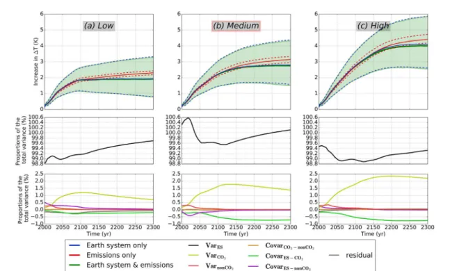
The upper panel of the figure 5 shows global sur-face temperature change with respect to the average of 1986–2005 (ΔT) simulated with OSCAR v2.2 and for the three future scenarios. In the Low, Medium and High scenarios, respectively, the 90% uncertainty

range of ΔT in 2100 due to uncertain Earth system parameters only are 1.1◦C–2.6◦C, 1.5◦C–3.0◦C and 1.9◦C–3.6◦C, with median values of 1.8◦C, 2.2◦C and 2.7◦C. With the uncertainty from fossil-fuel CO₂ and non-CO2emission parameters only, these ranges

are 1.8◦C–2.0◦C, 2.1◦C–2.4◦C and 2.6◦C–2.9◦C around 2100, which is about 6 times smaller than the Earth system uncertainty. When both the Earth system parameters and the emission parameters vary, the total uncertainty range remains very close to the case with varying Earth system parameters only. This

Environ. Res. Lett. 13 (2018) 044017

Figure 5. Upper panel: global surface temperature changes (in K) with respect to the average of 1986–2005 for the three extraction scenarios in the upper panels. The median and the 90% uncertainty range are shown for three experiments: with Earth system parameters varying (blue intervals), CO2and non-CO2emission parameters varying (red intervals), and both varying at the same time

(green plain line and shaded area). In the middle and lower panels, the variances and covariances identified are represented in terms of proportion of the total variance.

shows that the total uncertainty on ΔT is largely dom-inated by the Earth system uncertainty, despite an uncertainty of about 15% in cumulative CO₂ emis-sion estimates (figure 3), and uncertainties of up to a factor 2 for some non-CO₂ emissions (figure 4). This can be explained by the logarithmic relation of radiative forcing associated with CO₂with the atmo-spheric concentration of CO₂ (Myhre et al 1998). These results, summarized in table 5, also holds for the years 2200 and 2300. Besides, the ΔT obtained from the Low scenario are very close to the results for RCP4.5 from ESM (Knutti and Sedl´aˇcek 2012, Collins et al2013), the Medium scenario to RCP6.0 and the High scenario somewhat between RCP6.0 and RCP8.5. Knowing the correspondence of the three scenarios of extraction with the ones of RCP (figure 11 of Van Vuuren et al2011), and taking into account that the emissions from non-fossil fuels are prescribed here by RCP6.0, these projections in ΔT are consistent with the projections of RCP. The fact that the uncertainty in global mean temperature is dominated by the uncertainty in the Earth system’s response is consistent with Prather et al (2009) and Sokolov et al (2009).

In figure 5, using our 8 factorial simulations we attribute the variance of temperature change with all sources of uncertainty varying (green in figure 5) to variances and co-variances specific to uncertainties in the Earth system, fossil-fuel CO₂emissions and non-CO₂co-emissions. It is confirmed that the Earth system uncertainty largely dominates, since its attributed

variance stays around 100% of the total variance in the three scenarios.

The variance attributed to fossil-fuel CO₂ emis-sions peaks below 1.5%, 2% and 2.5% of the total variance in the Low, Medium and High scenarios, respectively; thus being quite negligible. The later CO₂ fossil-fuel emissions are peaking; the later the propor-tion of their associated variance peaks. Conversely, the co-variance attributed to the coupling of fossil-fuel CO2 emissions and the Earth system does not peak

at all. It increases (in absolute value) in all three sce-narios to reach respectively –0.2%, −0.7% and −0.8% by 2300. This negative co-variance reduces even fur-ther the importance of accounting for the uncertainty in fossil-fuel CO₂emission estimates at the same time as that in the Earth system’s response. The dampen-ing effect of the carbon cycle, that removes roughly half of yearly anthropogenic emissions from the atmo-sphere (Le Qu´er´e et al (2016)), explains this negative sign of the covariance between fossil-fuel CO₂emission uncertainty and Earth system uncertainty.

The variance attributed to non-CO2 emissions

present a similar profile in all three scenarios. It peaks at about 0.3% of the total variance, around 2025—a time at which it becomes less in magnitude than the variance attributed to fossil-fuel CO₂emissions. The shorter life-times for most of the non- CO₂species explains this decrease with time. The co-variance attributed to the coupling of non-CO₂emissions and the Earth system is the only one that appears to be scenario-dependent. In the Low and High scenarios, it decreases with time, 9

Table 5. Median and 90% ranges for the increase in global temperature with respect to the average of 1986–2005 (◦C), for the three scenarios of extractions and for the simulations with variations of the parameters relative to the emissions, or to the Earth system, or both. The relative uncertainties are given in parentheses. For comparison, the mean and ranges in 2100 of the RCP are given (based on a Gaussian assumption, by multiplying the multi-model standard deviation by 1.64).

Scenarios Simulations 2100 2200 2300

Scenario ‘Low’ Emissions (EXP3 1.9±0.1 (±6%) 2.1±0.1 (±6%) 2.3±0.1 (±5%)

Earch system (EXP4) 1.9±0.7 (±39%) 1.9±1.0 (±54%) 1.9±1.3 (±66%)

Emissions and Earch system (EXP7) 1.8±0.8 (±41%) 1.9±1.0 (±54%) 1.9±1.2 (±65%)

Scenario ‘Medium’ Emissions (EXP3) 2.2±0.1 (±6%) 2.9±0.2 (±6%) 3.1±0.2 (±6%)

Earth system (EXP4) 2.2±0.8 (±36%) 2.7±1.2 (±43%) 2.8±1.4 (±51%)

Emissions and Earth system (EXP7) 2.2±0.8 (±36%) 2.7±1.2 (±43%) 2.7±1.4 (±52%)

Scenario ‘High’ Emissions (EXP3) 2.7±0.2 (±6%) 4.1±0.2 (±6%) 4.4±0.3 (±6%)

Earth system (EXP4) 2.7±0.9 (±32%) 4.0±1.4 (±35%) 4.1±1.6 (±40%)

Emissions and Earth system (EXP7) 2.7±0.9 (±33%) 3.9±1.4 (±36%) 4.0±1.7 (±42%)

RCP2.6 0.9±0.7 (±73%)

RCP4.5 1.9±0.7 (±38%)

RCP6.0 2.3±0.8 (±34%)

RCP8.5 4.0±1.2 (±30%)

starting with a positive value in 2000 of 0.5% and 0.3%, respectively, of the total variance. In the Medium sce-nario, it is negative and peaks at about –0.4%. These various behaviors show the complex interplay between all the non-CO₂species, their timing of emission, and the Earth system’s response and various couplings and feedbacks.

The co-variance attributed to the coupling of CO₂ and non-CO2emissions remains negligible (<0.1%)

throughout all three scenarios. The residual term remains also negligible, except in the Low scenario. Because this scenario has less CO2emissions, it

indi-cates that the default configuration of OSCAR differs more from a hypothetical median configuration for processes related to non-CO₂species than for the car-bon cycle.

4. Discussion

A sensitivity analysis has been performed to evaluate the rule of the extension rule used to extrapolate the co-emission ratios (section 2.3), the background of non-fossil emissions and land-use change (section2.4) and the number of runs in the Monte-Carlo ensem-ble (appendix section 3). This analysis emphasizes our conclusions concerning the relative importance of the Earth system’s response and the emissions.

We use a global approach to estimate CO2

emis-sions and non-CO₂co-emissions trajectories based on global ‘emission factors’, and this can be deemed a caveat of our study. The use of national data, both for CO₂and co-emissions, would certainly provide more accurate estimates (Andres et al (2012)). However, in the dataset we use, the national data is expressed in terms of extraction, whereas the actual driver of emis-sion in a country is fossil-fuel consumption (Davis et al (2011). Going from the former to the latter requires trade data which is not available over distant peri-ods in the past, nor is it for the future. Although datasets of national fossil-fuel consumption do exist, they are not openly available (Speirs et al 2015).

Similarly, we use global instead of national NCVs, car-bon contents, and co-emission ratios, whereas these factors vary greatly among countries. Using national values for these factors would be possible, but it implies having a bottom-up approach based on fuel consump-tion data, for which fuels, emitting technologies and operating conditions should be distinguished, espe-cially for non-CO₂co-emissions (Peng et al2016). In this case, evaluating the resulting uncertainty would require a tremendous effort, in order to produce data that is not provided even by well-established inventories.

As explained in section 2.4, our produced emissions associated with fossil-fuel uses are included in broader sectors of the inventories. Energy uses of fossil-fuels are included in the energy sectors that often includes fossil sources and non-fossil sources. For this reason, the sum of our produced fossil-fuel emissions and the selection of non-fossil-fuels emissions from inventories are not strictly equal to the historical total emissions. This implies that our simulation over the historical period remains a scenario, and is no recon-struction of the historical climate change. However, the differences of our emissions to the inventories are close enough to extend our results to the historic period, and then to our scenarios.

Our approach allows us to combine the uncertainty in key parameters (energy or mass-based inventory method; carbon contents; fractions of oxidations; co-emissions) in an efficient manner without the need of making assumptions as to e.g. future use of emitting technologies. As we have shown that our calculated CO₂ and non-CO₂ global emission trajectories and uncertainties are comparable to exist-ing bottom-up data, we argue that our approach is good enough given the purpose of our investigation on the impact of uncertainty in fossil fuel emission estimates on projected climate change. Our study might overestimate the uncertainty in future non-CO₂ co-emissions, but this actually strengthens our con-clusion regarding the negligibility of this source of uncertainty.

Environ. Res. Lett. 13 (2018) 044017

We choose to present only the uncertainty anal-ysis for the global surface temperature as referred to in the UNFCCC. For the Earth’s surface temperature, the total radiative forcing and total annual precip-itation change, three global Earth system variables, which integrate the effect of various anthropogenic perturbations, we conclude that the emission-induced uncertainty is negligible. Not the uncertainty of CO₂ emissions, but the Earth system’s response variance contribute almost 100% to the change in global precip-itation in 2100 with respect to the average for 1986–2005 (appendix, figure 4.6).

However, for others variables such as the atmo-spheric CO₂concentration and the radiative forcing of CH4, of ozone, of aerosols and of black carbon, the

emission-induced uncertainty appears less negligible. In the High scenario, the atmospheric concentration of CO2in 2100 with respect to the average of 1986–

2005 reaches 352 ppm, with a range of 321–390 ppm (appendix, figure 4.1). This is about 42% of total uncer-tainty, which we attribute at 92% to the Earth system’s response in terms of variances. The uncertainty in CO2

emissions contributes with 8% to the total variance of atmospheric CO₂. The same relative importance of the uncertainty in CO₂emissions is observed for surface ocean pH. The change of the radiative forcing of tro-pospheric ozone in 2100 with respect to the average of 1986–2005 shows as well an uncertainty less neg-ligible. In the High scenario, it reaches 0.08 W m−2, with a range of 0.05–0.14 W m−2 (appendix, figure 4.3). The range induced by uncertain emissions rep-resents 43% of the range obtained with variations of all the parameters, emissions and Earth system. The range induced by the uncertain Earth system’s mod-elling reaches 86% of the range obtained with variations of all parameters. Radiative forcing of tropospheric ozone can be related to some extent to air quality issues (Crippa et al (2016), West et al (2013)). As shown in Saikawa et al (2017), uncertain emissions hamper air quality assessments. This calls for trans-parence and improvment of activity data and emission factors.

The different contributions to the total variance of the global surface temperature ΔT show partially compensating effects between all the species and com-ponents of the Earth system. Even though we can conclude that the uncertainty of anthropogenic fos-sil fuel emissions does not have a significant impact on the global temperature change, this is not the case for the impacts on atmospheric CO₂, ocean acidification or air quality.

5. Conclusions

We produced a distribution of historical CO₂ emis-sions from fossil-fuels with a relative uncertainty range of ±11%. Using broad fuel categories increase the uncertainty, because it masks the change in

composition of its fuels (e.g. hard coal, composed of anthracite, bituminous and subi-bituminous coals). Besides, the first resources depleted are conventional oil and gas and coals of good quality, leaving fos-sil fuels with stronger uncertainties on their carbon contents and net caloric values. Thus the uncer-tainty on fossil-fuel emissions is likely to increase with time. We have also produced three distributions of emission scenarios whose uncertainty reaches 15% in 2300 for cumulative emissions, and which have been complemented with non-CO₂ co-emission scenarios calculated using top-down estimates of co-emission ratios.

With the compact Earth system model OSCAR and a Monte Carlo setup, we have projected the global temperature change induced by these scenarios. Non-fossil-fuels emissions are provided by invento-ries on a slightly different sectoral basis, which does not hamper our conclusions. The relative uncertainty in these projections ranges from 42%–65%, and we have shown that the largest share is caused by the uncertainty in the Earth system representation. The uncertainty of anthropogenic emissions from fos-sil fuel represents only 6% of the variance of the system.

Our study shows that the global median temper-ature change induced by a given fossil fuel scenario is determined mainly by the uncertainty in the rep-resentation of the Earth system’s physical processes, and only for an insignificant part by the uncertainty in the estimate of fossil fuel emissions. However, the uncertainty of the fossil fuel emissions has a significant impact on the total variance for other species-specific Earth system variables, such as the atmospheric con-centration of CO₂ and the radiative forcing from tropospheric ozone. We also point out that this result may not apply locally, for variables such as precipitation.

Therefore, it remains important to keep improv-ing the emission factors used in emission inventories. For each existing category of fuel, the carbon content and net calorific value have to be periodically updated, to account for the variation in the mix of the fuels that compose it. Factors about non-conventional fuels need particular attention; and so do non-CO₂species (Li et al (2017), Li et al (2016)).

Acknowledgments

We thank Robert Andres for providing us with CDIAC data and information. We also thank Laurent Bopp for his help during the beginning of this study. We thank the reviewers for the constructive comments.

ORCID iDs

Y Quilcaille https://orcid.org/0000-0002-1474-0144

References

BP ( www.bp.com/en/global/corporate/energy-economics/statistical-review-of-world-energy/ downloads.html) (Accessed: 15 March 2018) EIA (www.eia.gov/cfapps/ipdbproject/IEDIndex3.

cfm?tid=90&pid=44&aid=8) (Accessed: 15 March 2018) IEA (www.iea.org/statistics/topics/co2emissions/) (Accessed: 15

March 2018)

US EPA 2012 National Emissions Inventory (NEI) Air Pollutant Emissions Trends Data, 1970–2012 Average Annual Emissions, All Criteria Pollutants ( www.epa.gov/air-emissions-inventories/air-pollutant-emissions-trends-data) (Accessed: 15 March 2018)

Allen M R, Stott P A, Mitchell J F B, Schnur R and Delworth T L 2000 Quantifying the uncertainty in forecasts of anthropogenic climate change Nature407 617

Andres R J et al 2012 A synthesis of carbon dioxide emissions from fossil-fuel combustion Biogeosciences9 1845–71

Arneth A et al 2017 Historical carbon dioxide emissions caused by land-use changes are possibly larger than assumed Nat. Geosci.

10 79–84

Boden T, Marland G and Andres R 1995 Estimates of global, regional and national annual CO2emissions from fossil-fuel burning, hydraulic cement production and gas-aring: 1950–1992 Technical Report, Carbon Dioxide Information Analysis Center, Oak Ridge National Laboratory, US Department of Energy, Oak Ridge, Tenn., USA, (NDP-O30/R6):600 (http://cdiac.ess-dive.lbl.gov/epubs/ ndp/ndp030/ndp0301.htm)

Boden T, Marland G and Andres R 2013 Global, Regional, and National Fossil-Fuel CO2Emissions (Oak Ridge, TN: Carbon

Dioxide Information Analysis Center, Oak Ridge National Laboratory, US Department of Energy) ( http://cdiac.ess-dive.lbl.gov/trends/emis/overview_2010.html)

Boden T, Marland G and Andres R 2017 Global, Regional, and National Fossil-Fuel CO2Emissions (Oak Ridge, TN: Carbon

Dioxide Information Analysis Center, Oak Ridge National Laboratory, US Department of Energy) ( http://cdiac.ess-dive.lbl.gov/trends/emis/overview_2014.html) Bond T C, Streets D G, Yarber K F, Nelson S M, Woo J H and

Klimont Z 2004 A technology-based global inventory of black and organic carbon emissions from combustion J. Geophys. Res. D Atmos.109 1–43

Clarke L E et al 2014 pp 413–510 Assessing transformation pathways. Climate Change 2014: Mitigation of Climate Change. Contribution of Working Group III to the Fifth Assessment Report of the Intergovernmental Panel on Climate Change 413−510 (www.ipcc.ch/pdf/assessment-report/ ar5/wg3/ipcc_wg3_ar5_chapter6.pdf)

Cofala J, Amann M, Klimont Z, Kupiainen K and

H¨oglund-Isaksson L 2007 Scenarios of global anthropogenic emissions of air pollutants and methane until 2030 Atmos. Environ.41 8486–99

Collins M et al 2013 Long-term Climate Change: Projections, Commitments and Irreversibility, Book Section 12 (Cambridge: Cambridge University Press) pp 1029–1136 (www.ipcc.ch/ pdf/assessment-report/ar5/wg1/WG1AR5_Chapter12_ FINAL.pdf)

Cox P and Stephenson D 2007 A Changing Climate for Prediction Science317 207–8

Crippa M, Janssens-Maenhout G, Dentener F, Guizzardi D, Sindelarova K, Muntean M, Van Dingenen R and Granier C 2016 Forty years of improvements in European air quality: regional policy-industry interactions with global impacts Atmos. Chem. Phys.16 3825–41

Davis S J, Peters G P and Caldeira K 2011 The supply chain of CO2

emissions Proc. Natl Acad. Sci.108 18554–9

EEA 2013 EMEP/EEA air pollutant emission inventory guidebook 2013: Technical guidance to prepare national emission inventories. EEA Technical Report, (12/2013):23 (www. eea.europa.eu/publications/emep-eea-guidebook-2013)

Flato G et al 2013 Evaluation of Climate Models, Book Section 9 (Cambridge: Cambridge University Press) pp 741–866 (www.ipcc.ch/pdf/assessment-report/ar5/wg1/WG1AR5_ Chapter09_FINAL.pdf)

Gasser T, Ciais P, Boucher O, Quilcaille Y, Tortora M, Bopp L and Hauglustaine D 2017a The compact Earth system model OSCAR v2.2: Description and -rst results Geosci. Model Dev.

10 271–319

Gasser T, Peters G P, Fuglestvedt J S, Collins W J, Shindell D T and Ciais P 2017b Accounting for the climate carbon feedback in emission metric Earth Syst. Dyn.8 235–53

Granier C et al 2011 Evolution of anthropogenic and biomass burning emissions of air pollutants at global and regional scales during the 1980–2010 period Clim. Change109 163–90

Hawkins E and Sutton R 2009 The potential to narrow uncertainty in regional climate predictions Bull. Am. Meteorol. Soc.90

1095–107

Hurtt G C et al 2011 Harmonization of land-use scenarios for the period 1500–2100: 600 years of global gridded annual land-use transitions, wood harvest, and resulting secondary lands Clim. Change109 117–61

IPCC 1996 Revised 1996 IPCC Guidelines for National Greenhouse Gas Inventories vol. 1–3 Intergovernmental Panel Climate Change (Paris: Organisation for Economic Co-operation and Development (OECD) and the International Energy Agency (IEA)) (www.ipcc-nggip.iges.or.jp/public/gl/invs1.html) IPCC 2006 2006 IPCC Guidelines for National Greenhouse Gas

Inventories vol. 1–5 2006 IPCC Guidelines for National Greenhouse Gas Inventories (www.ipcc-nggip.iges. or.jp/public/2006gl/)

Ito A and Penner J E 2005 Historical emissions of carbonaceous aerosols from biomass and fossil fuel burning for the period 1870–2000 Glob. Biogeochem. Cycles19 1–14

Janssens-Maenhout G et al 2015 HTAP-v2.2: A mosaic of regional and global emission grid maps for 2008 and 2010 to study hemispheric transport of air pollution Atmos. Chem. Phys.15

11411–32

Joint Research Centre 2011 EDGAR4.2: Emission Database for Global Atmospheric Research Global Emissions EDGAR v4.2 (https://doi.org/10.2904/EDGARv4.2)

Junker C and Liousse C 2006 A global emission inventory of carbonaceous aerosol from historic records of fossil fuel and biofuel consumption for the period 1860–1997 Atmos. Chem. Phys. Discuss.6 4897–927

Kirschke S et al 2013 Three decades of global methane sources and sinks Nat. Geosci.6 813–23

Knutti R and Sedl´aˇcek J 2012 Robustness and uncertainties in the new CMIP5 climate model projections Nat. Clim. Change3

369–73

Lamarque J F et al 2010 Historical 1850–2000 gridded anthropogenic and biomass burning emissions of reactive gases and aerosols: Methodology and application Atmos. Chem. Phys.10 7017–39

Le Qu´er´e C et al 2016 Global Carbon Budget 2016 Earth Syst. Sci. Data8 605–49

Li B et al 2016 The contribution of China’s emissions to global climate forcing Nature531 357–62

Li M, Klimont Z, Zhang Q, Martin R V, Zheng B, Heyes C, Cofala J and He K 2018 Comparison and evaluation of anthropogenic emissions of SO2and NOx over China Atmos. Chem. Phys.

1–28

Liu Z et al 2015 Reduced carbon emission estimates from fossil fuel combustion and cement production in China Nature524

335–8

Marland G, Hamal K and Jonas M 2009 How uncertain are estimates of CO2emissions? J. Ind. Ecol.13 4–7

Marland G and Rotty R M 1984 Carbon dioxide emissions from fossil fuels: a procedure for estimation and results for 1950–1982 Tellus B36 232–61

Meinshausen M et al 2011 The RCP greenhouse gas concentrations and their extensions from 1765 to 2300 Clim. Change109

Environ. Res. Lett. 13 (2018) 044017

Mohr S and Evans P G M 2010 Projection of world fossil fuel production with supply and demand interactions Chem. Eng. Depart. 783 21–171

Mohr S H, Wang J, Ellem G, Ward J and Giurco D 2015 Projection of world fossil fuels by country Fuel141 120–35

Moss R H et al 2010 The next generation of scenarios for climate change research and assessment Nature463 747–56

Myhre G, Highwood E J, Shine K P and Stordal F 1998 New estimates of radiative forcing due to well mixed greenhouse gases Geophys. Res. Lett.25 2715–8

Narayanan B G and Walmsley T L 2008 Global Trade, Assistance, and Production: The GTAP 7 Data Base, Center for Global Trade Analysis (Purdue University) (www.eea.europa.eu/ publications/emep-eea-guidebook-2013)

Novakov T, Ramanathan V, Hansen J E, Kirchstetter T W, Sato M, Sinton J E and Sathaye J A 2003 Large historical changes of fossil-fuel black carbon aerosols Geophys. Res. Lett.30 1–4

Olivier J, Muntean M and Peters J 2015 Trends in global CO2

emissions: 2015 report. PBL Netherlands Environmental Assessment Agency and European Commission’s Joint Research Centre (JRC) 1–78 (www.pbl.nl/en/publications/ trends-in-global-co2-emissions-2015-report)

Olivier J G J 2002 On the quality of global emission inventories. Approaches, methodologies, input data and uncertainties Thesis Utrecht University (https://dspace.library. uu.nl/handle/1874/678)

O’Neill B C, Kriegler E, Riahi K, Ebi K L, Hallegatte S, Carter T R, Mathur R and van Vuuren D P 2014 A new scenario framework for climate change research: the concept of shared socioeconomic pathways Clim. Change122 387–400

Peng S et al 2016 Inventory of anthropogenic methane emissions in mainland China from 1980–2010 Atmos. Chem. Phys.16

14545–62

Prather M J et al 2009 Tracking uncertainties in the causal chain from human activities to climate Geophys. Res. Lett.36 L05707

Riahi K et al 2017 The shared socioeconomic pathways and their energy, land use, and greenhouse gas emissions implications: an overview Glob. Environ. Change42 153–68

Saikawa E et al 2017 Uncertainties in emissions estimates of greenhouse gases and air pollutants in India and their impacts on regional air quality Environ. Res. Lett.12

065002

Sokolov A P et al 2009 Probabilistic forecast for twenty-first-century climate based on uncertainties in emissions (without policy) and climate parameters J. Clim.22 5175–204

Smith S J, Van Aardenne J, Klimont Z, Andres R J, Volke A and Delgado Arias S 2011 Anthropogenic sulfur dioxide emissions: 1850–2005 Atmos. Chem. Phys.11 1101–16

Speirs J, McGlade C and Slade R 2015 Uncertainty in the availability of natural resources: fossil fuels, critical metals and biomass Energy Policy87 654–64

Stern D I 2006 Reversal of the trend in global anthropogenic sulfur emissions Glob. Environ. Change16 207–20

Stohl A et al 2015 Evaluating the climate and air quality impacts of short-lived pollutants Atmos. Chem. Phys.15

10529–66

van Vuuren D P et al 2011 The representative concentration pathways: an overview Clim. Change109 5–31

Ward J D, Mohr S H, Myers B R and Nel W P 2012 High estimates of supply constrained emissions scenarios for long-term climate risk assessment Energy Policy51 598–604

West J J, Smith S J, Silva R A, Naik V, Zhang Y, Adelman Z, Fry M M, Anenberg S, Horowitz L W and Lamarque J-F 2013 Co-benefits of mitigating global greenhouse gas emissions for future air quality and human health Nat. Clim. Change3

885–9

Zhao Y, Nielsen C P, Lei Y, McElroy M B and Hao J 2011 Quantifying the uncertainties of a bottom-up emission inventory of anthropogenic atmospheric pollutants in China Atmos. Chem. Phys.11 2295–308