Active and passive separation control for drag reduction of a maneuvering hull form

Active and Passive Separation Control for Drag

Reduction of a Maneuvering Hull Form

bv

James Crandall Schulmeister

_{FEB 15 2017}

B.S., Yale University (2008)

_RARIES

S.M., Massachusetts Institute of Technology (2012)

Submitted to the Department of Mechanical Engineering in partial fulfillment of the requirements for the degree of

Doctor of Philosophy in Mechanical Engineering at the

MASSACHUSETTS INSTITUTE OF TECHNOLOGY

February 2017

@

Signature redacted

Author

...

Sin

t

r

e a t

d...

1"

Department of Mechanical Engineering

A November 29, 2016

Signature redacted

Certified by ... ...

Michael S Triantafyllou William I. Koch Professor of Marine Technology Thesis Supervisor

Accpte

Signature red acted

Accepted by ...

Sin

t

r

e

a t

d...

Rohan Abeyaratne, Quentin B rg Professor of Mechanics

Active and Passive Separation Control for Drag Reduction of a Maneuvering Hull Form

by

James Crandall Schulmeister

Submitted to the Department of Mechanical Engineering on November 29, 2016, in partial fulfillment of the

requirements for the degree of

Doctor of Philosophy in Mechanical Engineering

Abstract

Boundary layer separation is a source of large fluid dynamic forces on many engi-neered vehicles and structures, limiting the speed and efficiency at which we trans-port people and goods. The maneuvering of ocean and air vehicles in particular is limited by resistance due to cross-flow separation. Hull forms with lower hydrody-namic resistance in maneuvers are able to follow trajectories with tighter turns and at higher speeds. Despite the progress that has been made in the control of two-dimensional flow separation, little has been done to apply flow control to complex three-dimensional separation from maneuvering hull forms. This thesis studies and develops mechanisms for mitigating three-dimensional cross-flow separation to reduce the drag of hull forms in maneuvers.

A new strategy is proposed for designing flow control mechanisms for the three-dimensional flow past maneuvering hull forms based on the unsteady cross-flow anal-ogy. The unsteady cross-flow analogy relates the steady flow past a three-dimensional body to an analogous unsteady two-dimensional flow past a cylinder that changes size and shape in time. This provides a framework for adapting two-dimensional drag re-duction techniques to the three-dimensional flow. In addition, the unsteady cross-flow analogy is computationally inexpensive and so is suitable for iterative use in prelimi-nary design.

The new strategy is considered by first implementing the unsteady cross-flow analogy in numerical simulations. Next, passive and active flow control mechanisms are studied experimentally for drag reduction of a circular cylinder and then adapted through the analogy for drag reduction of a slender body at an angle of attack. Passive control is exerted through modifications to the shape of the body and active control is exerted with rotating control cylinders. Both passive and active methods are experimentally demonstrated to reduce the drag. The experimental results also confirm key predictions of the unsteady cross-flow analogy, demonstrating that it is a promising tool for developing three-dimensional separation control techniques.

Thesis Supervisor: Michael S Triantafyllou

Title: William I. Koch Professor of Marine Technology

Acknowledgments

I want to acknowledge the help of my advisor, Professor Triantafyllou. His insight, guidance, and support have been invaluable. I would like to acknowledge my the-sis committee members, Professor Yue and Professor Techet, for their constructive feedback and advice. I also want to acknowledge Professor Jason Dahl and Pro-fessor Gabriel Weymouth for their help and mentorship; I have very much enjoyed collaborating with them.

I must acknowledge the support and friendship of my labmates. I am grateful for many thought-provoking discussions at lunch and for always finding a willing ear for my questions about an experiment design or an aspect of hydrodynamics theory. I want to thank them, along with my family and friends outside of MIT, for lending moral support. I am grateful in particular for encouragement from my parents and the love and patience of my wife, Carrie.

Finally, I would like to acknowledge funding from NOAA's MIT SeaGrant program and the Singapore-MIT Alliance for Research and Technology (SMART).

Contents

1 Introduction

1.1 Thesis contributions and outline . . . .

1.2 Force coefficients . . . .

2 Unsteady Cross-Flow Analogy

2.1 Introduction . . . . 2.2 Background . . . .

2.2.1 Inviscid Models . . . .

2.2.2 Correcting for Viscous Effects with the Independence Principle 2.2.3 Unsteady Cross-Flow Analogy . . . .

2.3 Numerical Method . . . . 2.3.1 Implementing the Prolate Spheroid . . . . 2.3.2 Boundary Conditions . . . . 2.3.3 Grid and Domain Size Effects . . . .

2.3.4 Computing Normal Force and Moment . . . . 2.4 Prolate Spheroid . . . . 2.4.1 Review of Published Force Coefficients . . . . 2.4.2 Unsteady Cross-Flow Analogy Simulation Results 2.4.3 Location of Separation . . . . 2.4.4 Reynolds Number Effects . . . . 2.5 Limitations of the slender body methods . . . .

2.5.1 Limitations of inviscid slender body theory and independence principle . . . . 7 27 28 31 33 33 34 34 39 . . . . 45 . . . . 49 . . . . 49 . . . . 50 . . . . 53 . . . . 54 . . . . 56 . . . . 56 . . . . 58 . . . . 65 . . . . 70 . . . . 71 72

2.5.2 Limitations of the unsteady cross-flow analogy . . . .3

2.5.3 Possible improvements 2.6 Conclusion . . . . 3 Passive control of flow past a circular cylinder 3.1 Introduction . . . . 3.1.1 Background . . . . 3.1.2 Goals of this chapter . . . . 3.1.3 Designing the Shape Modification . . . . 3.2 Numerical simulations . . . . 3.2.1 Numerical method . . . .. . . . . 3.2.2 Numerical results . . . . 3.3 W ater tunnel experiments . . . . 3.3.1 Experimental method . . . . 3.3.2 Mean velocity field results . . . . 3.3.3 Force transducer results . . . . 3.3.4 Reynolds number effects . . . . 3.4 Conclusion . . . . 4 Passive control of flow past a prolate spheroid at an angle 4.1 Introduction . . . . 4.2 Unsteady Cross-flow simulations of modified spheroids . . . 4.2.1 Fixed aspect ratio elliptical cross-sections . . . . 4.2.2 Varying aspect ratio elliptical cross-sections . . . . . 4.2.3 Asymmetrically morphing cross-sections . . . . 4.3 Morphed spheroid experiments . . . . 4.3.1 Experimental method . . . . 4.3.2 Experimental results . . . . 4.3.3 Angle of attack effects . . . . of attack 105 . . . . . 105 . . . . . 107 . . . . . 107 . . . . . 110 . . . . . 115 . . . . . 119 . . . . . 120 . . . . . 128 . . . . . 142 145 4.4 Conclusion . . . . 8 . . . . 7 9 80 83 83 83 85 86 87 87 88 90 90 92 95 97 100 73

5 Active control of flow past a circular cylinder with rotating cylinders 149 5.1 Introduction . . . .

5.2 Experimental Method . . . . 5.3 Experimental Results . . . . 5.4 Numerical Method . . . . 5.5 Numerical Simulation Results . . . . 5.5.1 Wake Stabilization . . . .

5.5.2 Pressure Drag Reduction . . . . 5.6 Discussion . . . . 5.6.1 Mechanism of the Pressure Recovery 5.6.2 Pressure Recovery Scaling . . . .

. . . I . . . . 149 . . . . 153 . . . . 155 . . . . 157 . . . . 160 . . . . 160 . . . . 162 . . . 165 . . . 165 . . . 170 . . . 173 . . . 174

5.6.3 Power consumption of control with rotating cylinders 5.7 Conclusion . . . .

6 Active control of flow past a slender body at an angle of attack with rotating cylinders

6.1 Introduction . . . . 6.2 Experimental method . . . . 6.2.1 Slender body shape . . . . 6.2.2 Slender body model with rotating control cylinders . . . . 6.2.3 Rotating the control cylinders . . . . 6.2.4 Force measurements . . . . 6.3 Experimental Results . . . . 6.4 Conclusion . . . .

7 Conclusion

7.1 Thesis contributions . . . . 7.1.1 Unsteady cross-flow analogy . . . . 7.1.2 Passive control with morphing . . . . 7.1.3 Active control with rotating cylinders . . . . 7.2 Limitations of the proposed design strategy . . . ..

77 177 178 178 180 181 183 188 193 197 197 197 198 199 199 9

7.3 Future work . . . .. 200

A Potential Flow Models 203

A.1 Rotating Cylinder Flow Control ... 203

List of Figures

2-1 The prolate spheroid with fineness,

f

of attack of a = 300 (left). The slender body calculation is accurate for much of the body length, but fails near the ends. The moment is plotted as a function of the fineness,

f

in the cross-flow direction is independent from the streamwise direction. 40 2-4 Adapted from Allen (1949) [1]. The drag coefficient of a circular

cylin-der is smaller for lower aspect ratios. yq, the ratio of the drag coefficient of a finite cylinder to a an infinite cylinder monotoically approaches 1 as the aspect ratio increases. . . . . 44 2-5 The NACA vortex model diagram, adapted from Sarpkaya (66) [62]. 45 2-6 Unsteady cross-flow diagram. . . . .. . . . 46 2-7 The diameter of the circle in the unsteady cross-flow simulation varies

as an ellipse in time. The body starts and ends with a non-zero diamter, d = D/4, which smoothly transitions into and out of the elliptical

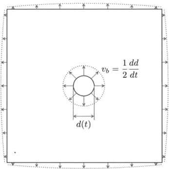
profile associated with the spheroid diameter along its span. . . . . . 51 2-8 The body's varying diameter in time requires new velocity boundary

conditions to be set at each time step on both the body and domain boundaries to permit incompressible flow . . . . . 52

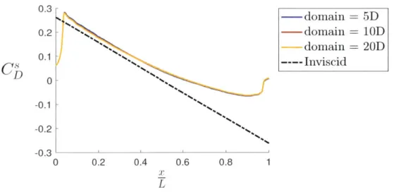
2-9 Effect of domain size on the cross flow force distribution. The grid

spacing was h = D/51.2 for these simulations. . . . . 53

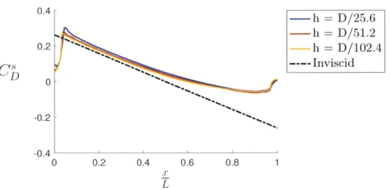
2-10 Effect of grid resolution on the cross flow force distribution. The do-main size was D/10 for these simulations. . . . . 54

2-11 Comparison of normal force distribution with experimental pressures [31] in the laminar boundary layer Reynolds number regime. The an-gles of attack are a = 60 (top), a = 100 (middle), and a = 20' (bottom). 59

2-12 Normal force distributions for a range of angles of attack computed with the present method implementation of the unsteady cross-flow analogy. The fineness ratio is 6. Chslender is Munk's inviscid slen-der body theory and CLIP is the independence principle cross-flow force using CD = 1 and added to the invsicid slender body prediction according to Allen [1]. . . . . 61

2-13 Sectional force coefficient normalized by sin(a) cos(a) collapses the po-tential theory to a single curve. The present Unsteady Cross-Flow Analogy method (UCFA) predicts a sectional force distribution that is biased toward the aft compared to the Independence Principle predic-tion (IP ). . . . . 62

2-14 Sectional force coefficient normalized by sin(a) cos(a) for low a. The present Unsteady Cross-Flow Analogy method (UCFA) predicts that at low angles of attack, the sectional force distribution collapses to a single curve and therefore the integrated normal force varies approximately

linearly with a. . . . . 62

2-15 Normal force coefficients for a range of angles of attack computed with the present method implementation of the unsteady cross-flow analogy. 63

2-16 Moment coefficients for a range of angles of attack computed with the present method implementation of the unsteady cross-flow analogy. . 64

2-17 This image is adapted from Wetzel and Simpson (1998) [83]. It shows separation lines estimated as the location of azimuthal minima of mea-sured skin friction. The angle of attack is a = 200 and the spheroid has fineness,

f

in the unsteady cross-flow analogy numerical simulations. . . . . 67 2-19 Separation location estimated using location of vanishing skin friction

in the unsteady cross-flow analogy numerical simulations. The sep-aration lines are projected onto a side view (top) and leeward view (bottom) of the 6:1 prolate spheroid. . . . . 68 2-20 Separation location estimated using location of vanishing skin friction

in the unsteady cross-flow analogy numerical simulations. The sep-aration lines are projected onto a three-dimensional rendering of the 6:1 spheroid for a = 10' (top), a = 20' (middle), and a = 300 (bot-tom). Slices showing contours of the cross-flow vorticity show that the separating helical vortices are leeward of the separation lines. . . . . . 69 2-21 The sectional force coefficient computed using the present unsteady

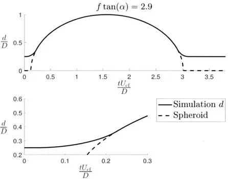
cross-flow method along with pressure measurements from Jones (1927) [31] for a = 6 and 10'. The unsteady cross-flow analogy predicts a small force near the finite ends where the diameter is smoothed to a finite value fo D/4. The "short smooth time" denotes a smoothing duration of 0.1 sin(a) and the "long smooth time" denotes a smoothing duration of 0.2 sin(a). . . . . 74

2-22 Normal force coefficient normalized by sin(a) cos(a). The present un-steady cross-flow analogy method does not converge to a horizontal line at low angles of attack as the experimental results of Wetzel & Simpson do. The present method decreases to values below the ON= 0.0012/0

curve reported by [21], maintaining a quadratic dependence on a even for a < 5'. The present method models the effects that are quadratic with a, but does not capture the linear effects at low a and high fineness. 77

2-23 Contours of

f

f

run. For example, the flow computed for an f = 5 spheroid at 100 is

equivalent to that for an

f

the same value of f tan(a). . . . . 78

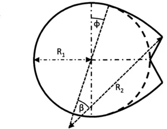
3-1 Diagram fo the modification to the circle. The modification is described by two parameters, R2/R1, and #. . . . . 87

3-2 Computational domain . . . . 88 3-3 The shapes that were tested in simulation with configurations listed

in table 3.1 are superimposed in dashed lines. The shape selected for

water tunnel testing is the solid black line (# = 0, R2/R1 = 4). . . . . 89

3-4 Photograph of 3D printed modified cylinder sheath installed on

alu-minum cylinder (left). Cylinder with sheath installed in the water

tunnel test section (right) spans nearly the entire test section to

miti-gate three-dimensional end effects . . . . 91

3-5 The mean streamwise velocity measured in coarse (arrows) and fine

(circle markers) grids behind the circular cylinder (black) and modified

shape (blue). At top, ReD = 32, 000 and at bottom, ReD 67, 000. . 93

3-6 The streamlines for the circular cylinder (top) and for the modified

shape (bottom). The Reynolds number was ReD = 32, 000. The heat

map shows the vorticity of the mean vorticity field. . . . . 94

3-7 Contours of the root mean square streamwise velocity for the circular

cylinder (top) and for the modified shape (bottom). The Reynolds

number was ReD = 32, 000. The modified cylinder reduces the

ampli-tude and region of fluctuating flow. . . . . 96

3-8 Mean drag coefficients measured with a strain gauge force transducer

for the circular cylinder and modified cylinder. . . . . 97

3-9 The root mean square lift coefficient for the circular cylinder and modi-fied cylinder. Similar to the drag coefficient presented in figure 3-8, the variation in the lift coefficient of the circular cylinder decreases with Reynolds number while there is no observable trend with Reynolds number for the modified cylinder. . . . . 97

3-10 The streamwise velocity profiles in the wake of the circular cylinder (top) and the modified cylinder (bottom) at ReD = 32, 000 and ReD -67,000. The velocity profiles for the modified cylinder at the different Reynolds nubmers are nearly identical, while the velocity deficit in the wake of the circular cylinder is greater at the lower Reynolds nubmer. 99

3-11 The power spectral density of the lift coefficient for the circular cylinder shows a peak at the frequency of vortex shedding. As the Reynolds number increases, the spectral peak at the vortex shedding frequency decreases in amplitude and becomes less coherent. . . . . 101

3-12 The power spectral density of the drag coefficient for the circular cylin-der shows a peak at the frequency of vortex shedding. As the Reynolds number increases, the spectral peak at the vortex shedding frequency decreases in amplitude and becomes less coherent. . . . . 102 3-13 The power spectral density of the lift coefficient for the modified

cylin-der. Compared to the spectra for the circular cylinder in figures 3-11 and 3-12, the spectral peak shows less variation with Reynolds number 103 3-14 The power spectral density of the drag coefficient for the modified

cylinder. Compared to the spectra for the circular cylinder in figures 3-11 and 3-12, the spectral peak shows less variation with Reynolds num ber . . . . 104

4-1 Diagram of the elliptical cross-section of the modified spheroid. The aspect ratio is equal to b/a, where b is the windward-leeward axis radius and a is the orthogonal axis. . . . . 108

4-2 The normal force distribution for ellipsoids with cross-sectional ellipses

of fixed aspect ratio along the length. Increasing the aspect ratio of the elliptical cross-sections reduces the normal force in regions where flow separation causes the force on the spheroid to deviate from the inviscid slender body theory prediction. . . . . 109

4-3 The normal force of ellipsoids varies with the aspect ratio of the cross-sectional ellipse, following the trend observed for two-dimensional el-liptical cylinders and reported by Hoerner [26]. . . . . 110

4-4 Diagram of collapsing as ellipse with varying aspect ratio. . . . . 111

4-5 Solid model rendering of the body with varying aspect ratio elliptical cross-sections. . . . . 112

4-6 The normal force distribution for a body with elliptical cross-section of increasing aspect ratio along the length compared to a spheroid for a = 100 (top) and a = 300 (bottom). . . . . 113

4-7 Normal force reduction of the body with ellitical cross-section of in-creasing aspect ratio along the length compared to the spheroid as a function of the angle of attack, a. . . . . 114

4-8 Normal force distributions for the spheroid show that the separation force starts in the fore half for a > 150 and in the aft half for a < 150. 115

4-9 Asymmetric morphing kinematics. As the projected area decreases, the center of mass of the cross-section moves leeward. . . . . 116

4-10 The normal force distribution for a body that morphs asymetrically in the aft, as shown in figure 4-9, is plotted along with the spheroid for a = 100 (top) and a = 30' (bottom). The asymetric morphing changes the inviscid slender body force prediction is included. . . . . 118

4-11 The normal force coefficients for the body that morphs asymmetrically in the aft are plotted with respect to a. Normal force coefficients for the body with elliptical cross-sections of increasing aspect ratio in the aft half from section 4.2.2 are also included. Both bodies are modified only for x/L > 0.5 and are spheroidal for x/L < 0. The reduction in normal force saturates for a > 150 for both bodies. . . . . 119

4-12 The morphed spheroid rendering shows the streamlining that is con-centrated in the aft half. The extension at the aft of 0.8 D, 1 D, 1.2

D, and 1.4 D measures the amplitude of morphing. . . . . 121

4-13 The morphed spheroid rendering shows the streamlining that is con-centrated in the aft half. . . . . 122 4-14 The raw data are tared and a linear trend is subtracted using the values

at the beginning and end of the test, during which times the flow is quiescent and the forces are therefore known to be zero. . . . . 124 4-15 The free stream velocity was increased in steps lasting 1 min each.

Data were sampled in 35 s windows at the end of each step after the flow had increased to the new commanded speed. . . . . 125

4-16 The spheroid model was towed using a rear-mounted sting along a straight trajectory at an angle of attack to the spheroid's longitudinal axis. The model's longitudinal axis was parallel to the long side of the tank and 2D planar PIV measurements were made in a plane normal to the spheroid's longitudinal axis and parallel to the short side of the

tank . . . . 127

4-17 Normal force coefficient measured in water tunnel tests with the models mounted at a = 15' (top) and a = 300 (bottom). Error bars for the spheroid measurements indicate the standard deviation of the force time series and are representative of the variance for the force on all models. Morphing reduces the normal force . . . . 129

4-18 Normal force coefficient measured in water tunnel tests with the models

mounted at a = 150 (top) and a = 30' (bottom). Error bars for the

spheroid measurements equal to the standard deviation of the force time series and are representative of all of the models. The potential flow moment experienced by the model, C1inviscid, comprises a larger

percentage of total measured moment at the lower angle of attack. . 131

4-19 The center of force on the spheroid at a = 300 can be estimated by comparing the measured moment in real flow to the inviscid prediction. The helical vortices that cause the normal force are larger and stronger in the aft, which causes the center of the normal force to also be biased

to the aft end at approximately x/L = 0.65. . . . . 133

4-20 Plotting the normal force and moment coefficients from the water tun-nel tests of the spheroid model shows that the two are highly

corre-lated. The moment the body would experience in inviscid flow, Miniscid

is subtracted from the measured moment. A fit line is plotted to show the linearity of the relationship between measured moment and normal

force. . . . . 133

4-21 Vortex reconstructions for the spheroid and shape 1 at a = 200. . 135

4-22 Vortex reconstruction for shapes 2 and 3 at a = 200. . . .. . . . . 136

4-23 Vortex reconstructions for the prolate spheroid as the angle of attack

increases: a = 10', 15 ,20 , 250 and 30 . . . . .. 137

4-24 Vortex reconstructions at a = 200 as the morphing amplitude increases. 138 4-25 Vortex reconstructions at a = 300 as the morphing amplitude increases. 139 4-26 The enstrophy is computed in a box that contains the cross-section

of the helical vortices, but excludes spurious measurements associated

with model and mount at the right side of the measurement window. 141

4-27 Repeatability of the enstrophy method is demonstrated by overlaying the enstrophy curves from multiple runs with the same model and angle

of attack. . . . . 142

4-28 Enstrophy curves for the spheroid at different angles of attack show the earlier development of the helical vortices and the greater energy contained in them . . . . . 143

4-29 Enstrophy curves for all of the models at a = 20' show the effect of the model geometry on the helical vortices. As the amplitude of the morphing increases, the enstrophy of the helical vortices decreases. . . 144

4-30 The enstrophy of the separating vortices at the aft end reflects the normal force on the model. The enstrophy increases with angle of

attack and decreases as the amplitude of morphing increases. . . . . . 145

4-31 The relative reduction in enstrophy of the helical vortices at the aft end of the model. Similar to the unsteady cross-flow simulations for shapes that have morphing limited to the aft half of the model, the reduction in force is greatest at low angles of attack and saturates above a critical angle of attack. . . . . 146

5-1 Diagram of the flow geometry. . . . . 153

5-2 Contours of mean streamwise velocity, u/Uo,, (left) from PIV measure-ments in water tunnel experimeasure-ments at ReD = 47, 000 with = 0 (top) and = 2.74 (bottom) show that rotating control cylinders reduce the streamwise momentum deficit. Streamlines of the mean flow (right) show that the rotating cylinders also narrow the wake. . . . . 156

5-3 The streamwise component of the velocity along the wake centerline (y/D = 0). The recirculation length decreases from 2.1D to less than 1.6D when the control cylinders are rotated with = 2.74. . . . . 156

5-4 In water tunnel experiments at ReD = 47, 000, the measured mean drag decreases with increasing control cylinder rotation parameter, ,

to 55% of the base flow drag when = 3.4. . . . . 157

5-5 Pressure profile (left) and normalized simulation error of the base pres-sure (right) for the configuration with g/D = 0.01, d/D = 0.01, and S= 4 with respect to grid resolution. The error is computed relative to the base pressure obtained using a fine D = 200h reference grid. The

solid line indicates second-order convergence with h and the dashed line indicates first-order convergence. . . . . 158

5-6 Streamlines for the viscous simulation (top) and a potential flow model (bottom) for rotation parameters, from left to right, = 2,3,4, and 5. For > 3, the viscous flow transitions from unsteady vortex shedding to a stable symmetric wake. The streamlines of the stabilized wakes approach the shape of those in the potential flow model. . . . . 161

5-7 Instantaneous vorticity contours from the ReD = 500 numerical sim-ulations for various rotation rates of the control cylinders. Higher rotation rates of the control cylinders stabilize and narrow the wake. . 161

5-8 The mean (solid line) and root mean square (shaded) pressure coeffi-cient along the main cylinder circumference as a function of the control cylinder rotation rate, , with g/D = 0.05 and d/D = 0.1. Above a critical rotation rate between = 2 and = 3, the fluctuations in the pressure profile are suppressed. . . . . 162

5-9 The pressure drag for the configurations with g/D = 0.05 decreases with the rotation parameter, . Larger diameter control cylinders achieve a greater drag reduction than smaller control cylinders at the same rotation rate. . . . . 163

5-10 The pressure recovery from separation to reattachment points is greater for larger control cylinders at the same rotation rate. . . . . 164

5-11 The pressure drag is correlated with the base pressure coefficient. . . 164

5-12 In the controlled steady flow, the pressure along the main cylinder presents two peaks associated with the separation and reattachment points of the dividing streamline. The rotating cylinder imparts energy to the fluid along the dividing streamline such that there is a pressure recovery, AC,, from separation to reattachment. . . . . 165

5-13 B, the total pressure or the sum of kinetic energy and pressure. At top, = 3 and at bottom, = 5. The wake recovery of B is greater

for higher . . . . 167

5-14 Net viscous shear power, P,, in the vicinity of the rotating control cylinder. The positive regions of P,, visible in the close view at bottom, are driven by the external forces required to keep the control cylinder in steady rotation. . . . . 168

5-15 The total pressure and viscous stress are plotted along the highlighted boundary layer streamline. Near the rotating control cylinder, B re-covers due to positive S ... . . . . 169

5-16 The pressure recovery from separation to reattachment of the dividing streamline (top) and from separation to the base of the cylinder at 0 = 7r (bottom), plotted with respect to the inviscid momentum flux scaling, d* (left) and the viscous momentum flux scaling, 3/2d*1/ 2

(right). The viscous scaling (right) more accurately describes the pres-sure recovery mechanism . . . . . 172

5-17 The pressure drag reduction, ACD,, increases with diminishing returns with respect to C;t. The most efficient configurations in this study are those with the smallest gaps between the main and rotating con-trol cylinders. At ReD = 500, all of the configurations are beneficial

(ACDP > C1"). The CT = Crtt line indicates the maximum physi-cally possible drag reduction. . . . . 174

6-1 The slender body shape is a piecewise combination of a spheroid in the fore and a cone in the aft. The cone is amenable to rotating cylinder flow control because the control cylinders can be installed with a small

gap to the body along their length. . . . . 180 6-2 The model was constructed as a hollow shell in two halves. Internal

flexure mounts enabled the model to be fixed to the rear sting. . . . . 181 6-3 The rotating cylinders smoothly emerged from the body of the model

without any upstream protruding bearing surfaces that might cause the flow to separate. . . . . 182 6-4 The model installed in the water tunnel is shown. The model, rotating

cylinders, rear sting, shaft coupler, force transducer, and flexible drive shafts are called out in the figure. . . . . 183 6-5 A linear drift is subtracted from the raw signals. . . . . 185 6-6 In each test the rotation rate of control cylinders is constant. The free

stream is initially quiescent, accelerated to the test value, during which samples are recorded in the sample window, and then decelerated back to quiescent. . . . . 187 6-7 In these tests the rotation rate of the control cylinders is held constant

for the duration of a test while the free stream velocity is stepped through multiple values. As a result, each step corresponds to a differ-ent rotation parameter. At each step the forces are sampled for a 35 s

w indow . . . . 188

6-8 The mean moment coefficient, C1, for tests using 250 s and 35 s sample windows at a = 30' are compared. The magnitude and variance of the measurements are comparable, indicating that the 35 s sample window is sufficiently long to accurately measurement the moment. . . . . 189 6-9 The moment coefficient, Cm, with = 0, shows a decreasing trend

with ReL at a = 300. The observed decreasing trend indicates that the flow is transitional. In contrast, the a = 15' show no trend with

R eL . . . . 190

6-10 CM is plotted with respect to for the a = 300 tests. In the top plot, the data are marked according to the rotation rate of the control cylinders in RPM. In the middle plot, the data are marked according to ReL. The bottom plot normalizes each datum by the value at the same ReL and = 0. . . . . 191 6-11 CM is plotted with respect to 6 for the a = 15' tests. In the top

plot, the data are marked according to the rotation rate of the control cylinders in RPM. In the middle plot, the data are marked according to ReL. The bottom plot normalizes each datum by the value at the same ReL and 6 = 0. . . . . 192 6-12 Relative reduction of CM with rotation parameter, , and the

effec-tive rotation parameter, / sin (a). The data from the two angles of attack are more tightly collapsed with respect to the effective rotation param eter. . . . . 194

List of Tables

3.1 Simulated pressure drag coefficients, CDP, for a range of shape param-eters, < = 0' and R2/R1 . . . . 90 5.1 Configurations tested in the water tunnel experiments (22 in total). . 154 5.2 Configurations of the numerical simulations (60 in total). . . . . 160

Chapter 1

Introduction

Boundary layer separation is a source of large fluid dynamic forces on many engineered vehicles and structures, limiting the speed and efficiency at which we transport people and goods. These mitigation strategies include flow control, which operates through targeted momentum injection.

The maneuvering of ocean and air vehicles in particular is limited by resistance due to cross-flow separation. A ship's motion is the result of the sum of forces exerted on it, including forces due to its propulsion, control surfaces, and hydrodynamic forces on the hull. Hull forms with lower hydrodynamic resistance in maneuvers are able to follow trajectories with tighter turns and at higher speeds. Maneuverability, the capability to change speed and direction rapidly, is an important aspect of ship performance.

Despite the large body of work developing flow control for cylinders and many promising results [17], there are yet very few successful demonstrations of flow control applied to reducing the resistance of maneuvering hull forms, even at the laboratory scale. Compared to cylinders, a maneuvering hull form's three-dimensional flow is topologically complex. In addition, studying three-dimensional flows, both in ex-periment and in simulation, are measurement- and computationally expensive. The added complexity and cost compared to cylinder flows make for a daunting design problem, which has likely contributed to the scarcity of work on the topic.

This thesis proposes a, new strategy for designing flow control mechanisms for 27

the three-dimensional flow past maneuvering hull forms based on the unsteady cross-flow analogy. The unsteady cross-cross-flow analogy relates the steady cross-flow past a three-dimensional body to an analogous unsteady two-three-dimensional flow past a cylinder that changes size and shape in time. The proposed strategy involves applying flow control mechanisms for two-dimensional cylinders to the unsteady cross-flow representation of a three-dimensional hull form in numerical simulations. This provides a framework for adapting two-dimensional techniques to the three-dimensional flow. In addition, the unsteady cross-flow analogy is computationally inexpensive and so provides an efficient modeling tool that can be used iteratively in preliminary design. It is hoped that this design strategy will provide a starting point from which the rich body of cylinder flow control work can be extended to the three-dimensional manuevering hull form.

1.1

Thesis contributions and outline

Of the many flow control mechanisms investigated in the literature, two were consid-ered in the development of the proposed design strategy: one passive and one active. The passive mechanism uses control surfaces to modify the shape of or morph the body. Morphing changes the body surface pressure gradients to influence the sep-aration. This passive technique is analogous to wing flaps, the deflection of which change the camber of the wing and thereby its force coefficients. The active mecha-nism is Moving Surface Boundary layer Control (MSBC) implemented with rotating cylinders. The no-slip condition of the moving surface of the rotating cylinder injects momentum into the flow to mitigate separation. Rotating cylinders are classified at "active" because power is required to operate them. A shape modification, once deployed to a static position, does not consumer power to operate and is classified, "passive".

This thesis presents three key contributions to the application of flow separa-tion control to reduce the forces on hull forms in steady turning. The first key contribution is an analysis of the unsteady flow analogy for modeling the

flow separation past slender bodies at an angle of attack. Chapter 2 presents a method for implementing the unsteady cross-flow analogy in numerical simulations of the two-dimensional Navier-Stokes equations using the Boundary Data Immersion Method (BDIM) [86, 43]. The method is analyzed by modeling the flow past a prolate spheroid at an angle of attack and comparing the results to published measurements. The prolate spheroid is representative of many hull forms and is commonly used in the literature. The method is found to provide satisfactory predictions of the location of separation and the distribution of the lateral force on the spheroid with computa-tional cost several orders of magnitude less than high fidelity methods. Limitations of the analogy are also discussed.

The second key contribution is the development of passive shape modifications to a prolate spheroid that reduce the normal force at an angle of attack. Chapter 3 investigates this control mechanism for the two-dimensional flow past a circular cylinder. Design constraints related to the realization of the morphing with actuated control surfaces are established and a suitable geometry is selected through a series of numerical simulations. Water tunnel tests of a model of the designed geometry show that the passive mechanism reduces the drag of a circular cylinder by more than 50%. Chapter 4 extends the passive control mechanism to the prolate spheroid. First, the unsteady cross-flow method developed in chapter 2 is used to explore three mor-phing effects. These include mormor-phing the spheroid to have elliptical cross-sections with fixed aspect ratio along the length, to have elliptical cross-sections with vary-ing aspect ratio along the length, and to have cross-sections with windward-leeward asymmetry. These represent, respectively, effects related to the amplitude of morph-ing, the axial distribution of morphmorph-ing, and morphing that also changes the location of the cross-sectional center of mass. A class of shapes combining these effects is then designed for testing. Tow tank and water tunnel tests of the designed models demonstrate the reduction of the normal force by up to 40%. The separating helical vortices are reconstructed from PIV measurements in tow tank tests to illustrate the effect of the morphing on the flow.

The third key contribution is a new description of the separation control mech-29

anism of rotating control cylinders and its application to cross-flow separation of a slender body at an angle of attack. Chapter 5 presents an experimental demonstra-tion of flow control with rotating cylinders in water tunnel tests at ReD = 47, 000. The measured drag reduction of 45% is significant because it is demonstrated at a higher Reynolds number than similar studies in the literature. The configuration parameters are also investigated in numerical simulations. These simulations are the first to investigate the role of the diameter of the control cylinder in addition to its rotation rate and gap to the main cylinder. The drag reduction is found to scale with the momentum flux of the control cylinder associated with its viscous boundary layer as opposed to its circulation. This viscous scaling is an advancement in the understanding of the rotating cylinder control mechanism, which has previously been attributed only to the circulation [46].

Chapter 6 adapts the rotating control cylinder mechanism to the flow past a slender body at an angle of attack. A special slender body is designed to accommodate the rotating cylinders. Water tunnel tests of the rotating control cylinder-equipped model showed that the normal force can be reduced by more than 20% at an angle of attack of a = 30' and by more than 40% at a = 150. This laboratory scale demonstration of normal force reduction of a slender body with active flow control is significant because it is the first of its kind. In addition, the relative reduction of the normal force collapses with respect to an effective rotation parameter defined with the cross-flow component of the free stream velocity. This observation supports the use of the unsteady cross-flow analogy in preliminary design.

This thesis advances the state of the art in flow control for hull forms by demon-strating that both passive and active mechanisms for a two-dimensional circular cylin-der can be adapted to reduce the normal force on slencylin-der bodies at an angle of attack. The design adaptation is accomplished through the unsteady cross-flow anal-ogy, which maps the three-dimensional flow to an unsteady two-dimensional flow. In comparison, the independence principle is found to be insufficient in predicting the development of separation and distribution of force, which are important aspects of flow control. In other words, the unsteady cross-flow analogy is suitable for

liminary design of three-dimensional flow control while the independence principle is not.

1.2

Force coefficients

In this thesis, two dimensional force coefficients are reported using the stagnation pressure of the free stream, q = 1/2pU., and the projected area, S. The projected

area for a circular cylinder with diameter, D, and span, L, is S = DL. The drag

force, FD, is parallel to the free stream, and the lift force, FL, is orthogonal to both the cylinder span and the free stream.

FL FD

CL = , CD =q

(-qS qS

For three-dimensional bodies, including the prolate spheroid, the normal force, N, is of primary interest because it does work to slow the vehicle in maneuvers. The normal force, sometimes refered to as the lateral force, is orthogonal to the slender body's longitudinal direction. This is distinct from the lift, which is orthogonal to the free stream or body translation. The longitudinal direction of a prolate spheroid is its axis of revolution. Measured force coefficients are compared to published results for fineness ratios within 4 < f < 6. The normal force coefficient is roughly constant for similar shapes over a wide range of fineness ratios when defined using the projected area [26].

CN = (1.2)

qS

The normal projected area of a prolate spheroid is S = rab, where a and b are,

respectively, the minor and major radii of the revolved ellipse. The fineness is the ratio between these,

f

also be written using the maximum diameter, D, the length, L, and the fineness,

f,

asS = !D 2f.

to maintain stable motion. The moment coefficient is defined using a characteristic volume. In this thesis, the moment coefficient for the prolate spheroid is presented using the volume of the spheroid, V = 2D3_f.

M

CM = (1.3)

Chapter 2

Unsteady Cross-Flow Analogy

Abstract

This chapter provides background on modelling techniques for predicting the forces and moments on slender bodies moving at an angle of attack in incompressible flow. One of these, the unsteady cross-flow analogy, is implemented with numerical simula-tions of the two-dimensional Navier-Stokes equasimula-tions. The flow past prolate spheroids at a range of angles of attack are computed and the results show good agreement with published numerical and experimental results, both for integrated force coefficients and the longitudinal distribution of the normal force. These simulations are much less computationally expensive than full three-dimensional simulations, making them a useful tool in preliminary design of flow control techniques.

2.1

Introduction

Much of the research work developing models of the flow past slender bodies at an angle of attack has been motivated by the need to predict the forces and moments on air and ocean hull-forms and slender body projectiles. Accurate predictions of forces during maneuvers is important for designing control surfaces to meet stability, propulsion, and maneuvering performance specifications.

Engineers now have the tools to model the full three-dimensional flow in numerical simulations, but these are computationally expensive. Simulation times typically scale with the number of cells and time steps at which the equations of motion are solved. For example, the simulations reported in chapter 5, use 106 cells (1,000 nodes span

each side of the square domain) to simulate the two-dimensional flow past a circular cylinder at ReD= 500. A corresponding three-dimensional simulation would require O(10') cells and incur a roughly 1,000 times increase in simulation time. Increasing

the Reynolds number would require further increases in grid and time resolution. As a result, the brute-force parameter exploration approach taken in chapter 5 is not feasible to study flow control of three-dimensional separation.

In addition to the computational cost incurred to numerically simulate three-dimensional flows, the parameter space describing possible flow control actuators is much broader than in two-dimensional flows; actuators direct momentum injection in three instead of two dimensions and are distributed over a surface instead of a curve. A consequence of these difficulties is that few studies tackle three-dimensional separation control. In contrast, there is large volume of published work investigated flow separation control strategies for flow past two-dimensional cylinders and airfoils. Inexpensive approximate modeling methods are valuable tools in preliminary de-sign because they can be used iteratively. This chapter presents an implementation and analysis of one such approximate technique, the unsteady cross-flow analogy. De-spite its simplifications, the analogy nevertheless captures much of the physics of flow separation past slender bodies at an angle of attack, measured by the predicted forces and moments. This analysis supports the use of the unsteady cross-flow analogy as a tool for designing slender body separation control mechanisms.

2.2

Background

2.2.1

Inviscid Models

Most modeling techniques were analytical and based on potential flow theory until the late 1940's [32]. According to potential flow theory, the fluid force on a body moving at a steady velocity is equal to zero. That this result is inconsistent with the resistance of vehicles and projectiles observed in real fluid flows is known as d'Alembert's Paradox. Potential theory does not model viscous effects, including boundary layers and flow

separation, that create resistance in steady flows of real fluid. Desoute tgus limitation, potential theory makes accurate predictions at low angles of attack of slender bodies in which flow separation does not occur over the majority of the body. Potential theory also incurs low computational cost and analytical results are often simple enough for engineering use.

Munk (1924) presents an expression for the hydrodynamic moment experienced

by bodies of revolution when subject to ideal streaming flow at an angle to the

body's axis of revolution. Munk's expression, known as the "Munk Moment" (2.1), elegantly relates the moment to a simple function of the added mass of the body in the longitudinal and transverse directions [51]. Here, Kip and K2p are the added masses

in the direction of the axis of revolution and an orthogonal direction, respectively, and q = ipU2 is the free stream stagnation pressure.

M = q(K2 - K1) sin(2a) (2.1)

This expression is exact for potential flow and is equivalent to integrating the potential flow solution pressure over the entire surface area of the body. The "Munk Moment" is more convenient than integrating the pressure because the added mass coefficients for slender hull-form bodies can often be easily estimated analytically using strip-theory [52]. Or, as Munk suggests, the added mass coefficients can be approximated as those of an ellipsoid, which are known analytically [42], with the same length and volume.

Munk also presented an approximate calculation for the sectional normal force distribution for "very elongated airships". Munk asserts that when the body is elon-gated, the flow in the longitudinal direction can be neglected and so the flow in planes normal to the body longitudinal axis is nearly two-dimensional. The flow in each plane can therefore be estimated as the two-dimensional flow past the cross-sectional shape of the body. The body has a different size cross-section at each station from the fore to aft, so the two-dimensional cross-flow of a body of revolution is analogous to one past a circle that translates while growing and shrinking as the body cross-section

changes along its axis of revolution. The circle translates at the cross-flow velocity,

U, sin(a). The rate of change of the diameter, d, in time is a function of the axial

rate of change of the diameter, dd/dx. Here, x is the coordinate along the body axis of revolution.

dd dddx dd

- =--= U0 cos(a) _(2.2)

dt dx dt dx'

The force in the cross-flow plane, F', which corresponds to the sectional normal force per unit length on the body of revolution, is equal to the time derivative of the fluid momentum in the cross-flow plane. The cross-flow fluid momentum around a circular cross-section is equal to pUm sin(a)7r/4d2_{, so}

Fs = U, sin(a) cos(c)dj. (2.3)

2 00dx

A sectional drag coefficient can be calculated by normalizing this force by the free

stream stagnation pressure and the maximum cross-sectional diameter, D.

FS ddd

CL = 1 UFD = 7r sin(a) cos(a) (2.4)

2pU2cD D dx

It is helpful to consider an example to see the differences between this slender body theory and the three-dimensional potential flow theory. Let's consider the prolate spheroid, which is the surface formed by revolving an ellipse about its major axis. A prolate spheroid with fineness, f = 5, is rendered in figure 2-1. The diameter, d(x),

for a prolate spheroid with fineness,

f,

d(x) D2 - ( 2 (2.5)

Substituting the spheroid (2.5) into (2.4), the slender body sectional force coeffi-cient is found to vary linearly along the longitudinal axis.

-47r

CL(spheroid) = sin(a) cos(a) - (2.6)

Figure 2-1: The prolate spheroid with fineness,

f

used shape in the literature to represent submarine hulls.

The slender body sectional force coefficient is shown in figure 2-2, along with the three-dimensional potential flow solution computed using a panel method. The linear normal force distribution predicted by the slender body theory matches the three-dimensional potential flow solution well over the majority of the body, but fails near the ends. In three-dimensional flow, fluid can move around the finite ends and the slender body assumption is not valid. It is apparent in the force distribution that the slender body theory will overestimate the moment on the body. Munk suggests that, for engineering purposes, the slender body prediction could be multiplied by a factor,

(K2 - K1), where Kip and K2p are the added masses in the direction of the axis of

revolution and an orthogonal direction, respectively. This factor incurs greater error in the middle of the body, but, when integrated along the length, accurately predicts the moment. This correction is labeled "Slender Body with Correction" in figure 2-2. The moment coefficient predicted by the slender body theory, CM(slender), is found by integrating the moment of sectional force. This is computed below for the spheroid in (2.7).

fL2ChqDxdx

SL/2

CM(slender) = J-L/2 = sin(2a) (2.7)

0.25

-0.5

--3D Potential Flow - - - - -- --Slender Body 0.2 -

---- Slender Body with Correction

0.15- /

C;, CAIj

0.1

-3D) Potential Flow - - Slender Body Theory

0.05 Strip Theory

Hoerner'sCorrection

-0.5 0

-0.5 0 0.5 0 2 4 6 8 10

x/L _f

Figure 2-2: Normal force distribution for an

f

attack of a = 300 (left). The slender body calculation is accurate for much of the body length, but fails near the ends. The moment is plotted as a function of the fineness,

f

Consistent with the assumptions of slender body theory, the computed moment coefficient is independent of the fineness ratio. This non-dependence on fineness is inaccurate because the added mass terms in Munk's moment expression (2.1) change with the fineness ratio. The error of the slender body theory prediction approaches zero as the fineness increases. This is illustrated in the right plot of figure 2-2 in which the moment coefficient by three-dimensional potential theory and slender body theory are plotted as a function of the body fineness ratio.

A heuristic correction from Hoerner as well as the moment computed using added

mass coefficients estimated with strip theory are also included in figure 2-2. Hoerner's correction (2.8) ensures that the moment is zero for f = 1 (sphere) and equal to the slender body theory limit as

f

Cm = Cm(slender) 1 - (2.8)

The strip theory estimate of K2 is computed by treating each section of the body normal to the longitudinal axis as two-dimensional and integrating the contribution of each strip to the added mass of the three-dimensional body. Here, K2D (x) is the

two-dimensional added mass coefficient of the cross-section shape at a distance x from the center of the body.

K₂strip = -L2 K ₂D(x)dx (2.9)

The two-dimensional added mass coefficient of a circle is equal to the area of the circle, K2D =1/47rD2, so the strip theory computation is equal to the volume of the spheroid.

K2s, = V (2.10)

The exact value for the longitudinal added mass coefficient for a prolate spheroid,

K1 = 1/127rD3, is used for the strip theory moment calculation plotted in figure 2-2.

The strip theory estimate is inaccurate for low fineness spheroids where end effects are more pronounced, but has smaller error than Hoerner's correction for higher fineness

spheroids. The error of all of the methods approach zero as

f

2.2.2

Correcting for Viscous Effects with the Independence

Principle

In flows of real fluid, flow separation alters the flow and resulting forces and moments significantly compared to the inviscid models. Flow separation is a viscous effect because it occurs due to the evolution of a viscous boundary layer in an adverse pressure gradient. Despite being a viscous effect, flow separation alters the forces and moments on a body predominantly by changing the pressure distribution as opposed to shear stress. Viscous effects (separation) become important at angles of attack as

low as 5'. Many vehicles experience flow at angles of attack up to 300 or greater in

normal operation, so accurate estimates of the viscous effects are relevant to normal operation.

An engineering method for predicting the viscous effects of the flow past a slender body at incidence was proposed by Allen [1, 2]. Allen's method is based on an assumption that the normal force on a slender body, Fs, can be decomposed into independent potential flow, F8, and viscous flow, F,' contributions that are summed

A

U00 cross flow

spanwise

Figure 2-3: The Independence Principle states that flow past an inclinded cylinder in the cross-flow direction is independent from the streamwise direction.

together.

FS = Fs + Fs (2.11)

The potential force term, F", is computed using the inviscid slender body theory method of Munk described in section 2.2.1, and the viscous force term, F,, is esti-mated using empirical data of cylinders in streaming flow normal to the cylinder span combined with the independence principle or cosine law.

The independence principle states that in the flow past an inclined cylinder, the flow components in the normal and spanwise directions of the cylinder are independent

[93]. Accordingly, the normal force, vortex shedding frequency, etc., can be computed

from results of flow normal to the cylinder by re-normalizing to the cross-flow velocity,

Ucf = U. cos(A), thus the alternative name, cosine law. A diagram of a cylinder inclined to a streaming flow is shown in figure 2-3. The inclination angle, A, measures the inclination of the cylinder axis from encountering a normal streaming flow.

Experiments supporting the independence principle were first published in 1917

[61], though its theoretical basis was not described until later by Prandtl (1946), Sears

(1948) [78], and others. The theoretical treatment applies Prandtl's arguments for the magnitude of laminar boundary layer quantities in the Navier-Stokes equations

for incompressible flow. Neglecting terms of the order of the boundary layer thickness results in equations of motion of the cross-flow boundary layer that are identical to those for a cylinder in normal flow. These arguments are reproduced briefly below.

Following Sears [78], a curvilinear coordinate system is defined in which x is tangent to the cylinder and z is normal to the cylinder surface. The coordinate parallel to the cylinder axis is y. The velocity component in the (x, y, z) directions are represented by (u, v, w). The cylinder has constant cross-sectional shape and infinite span, so none of the quantities vary with y. The continuity equation and equations of motion after neglecting derivatives with respect to y become:

u u OW + += 0+

ax

19z

OU

au

OU

av

OV

at

ax

Ow +w

The boundary conditions are that all components of the velocity vanish on the cylinder surface and are equal to the inviscid solution values at the outer edge of a thin boundary layer with thickness, 6 << L, where L is the length scale of the cylinder cross-section. Since the boundary layer is thin, within the boundary layer au/Oz is

0(1/6) and a2u/0z2 _is

0(1/62), etc. From continuity (2.12), within the boundary

layer Ow/Oz is 0(1), and so w is 0(6). Removing terms from (2.12 - 2.15) that are

0(6) and smaller results in the yawed cylinder cross-flow boundary layer equations.

(2.12)

(2.13)

(2.14)