An approach to the preliminary design of controlled structures

(1)

An Approach to the Preliminary Design of

Controlled Structures

by

Robert Normand Jacques

S.B. Massachusetts Institute of Technology (1988)

SUBMITTED TO THE DEPARTMENT OF AERONAUTICS AND ASTRONAUTICS

IN PARTIAL FULFILLMENT OF THE REQUIREMENTS FOR THE DEGREE OF

Master of Science in

Aeronautics and Astronautics at the

Massachusetts Institute of Technology February 1991

©

Signature of Author V- - Cý - t

D, I~ment of Aeronautics and Astronautics February 11, 1991

Certified by

Accepted by

Professor Edward F. Crawley Thesis Supervisor, Depart-e nt of Aeronautics and Astronautics

rofessor Harold Y. Wachman Chairman, Department Graduate Comittee

MASSACHUSMS IVSTIIuTe_{OF TECHNot}_nGy

FEB 19 1991

LIBRARIES

(2)

An Approach to the Preliminary Design of Controlled Structures

by

Robert Normand Jacques

Submitted to the Department of Aeronautics and Astronautics on February 11, 1991 in partial fulfillment of the

requirements for the Degree of Master of Science in Aeronautics and Astronautics

Abstract

Current trends in flexible space structures often place many flexible modes of the spacecraft inside the bandwidth of active controllers required to meet pointing and align-ment requirealign-ments. To properly design these structures, the presence of active control must be taken into account. The current approach to this problem has been to optimize the structure and the control of the system simultaneously. However, this methodology suffers from the fact that numerical optimization provides the engineer with very little insight into the problem. This insight is crucial in the early stages of design of the controlled structure. Even in cases where numerical optimization is to be used, it is necessary to have a basic understanding of the problem in order to properly select the design variables.

This work seeks to rectify this problem. Five mechanisms for improving the perfor-mance of a controlled structure were identified. These were disturbability, controllability, observability, open-loop dynamics, and robustness. These terms described the infuence of the disturbance on the system, the influence of the control on the system, the influence of the system on the performance output, the effects of natural frequency and damping, and the effects of poor modelling.

A series of simple problems were solved which show how the relative improtance of each of these quantities changes as the problem definition changes for different types of disturbances, performance outputs and control levels. The analysis leads to a set of design rules which should be useful in preliminary design. The gradients are found for arbitrary systems and are broken down into subgradients so that the relative importance of the five mechanisms can be tracked in more complex system optimizations. The design rules, in conjunction with the insight obtained from the subgradients are used to interpret optimization results in this thesis and other research.

Thesis Supervisors: Edward F. Crawley, Sc.D. David W. Miller, Ph.D. Professor of Research Associate

(3)

Acknowledgements

I owe a great deal of thanks to many people in connection with this work. First, I would like to thank my advisor, Dr. David Miller. He was was present at every step of the process. Many of the ideas expressed here originated from Dr. Miller, and his editorial comments helped ensure that this thesis reached completion. I would also like to thank Professors Edward Crawley and James Marr. They saw the need for work in this area and provided the initial direction. Credit should also go the other graduate students in SERC, particularly Farla Fleming. Conversations with them helped clarify many points.

Finally, I would like to thank someone who I am sure I have slowly driven crazy over the past few months. To my wife, Evelyn, your patience helped me over some rough spots, and your prodding got me out of some ruts.

(4)

Chapter 1 Introduction to Controlled

Structure Optimization

Lately, there has been a great deal of interest in methodologies which can be used to design the structural and control subsystems of large space structures simultaneously. Traditionally, the design of these subsystems has been performed separately, with the control design occurring long after the structural design has been completed. This method worked quite well when structures were smaller and relatively stiff. Most, if not all, of the flexible modes of these spacecraft were well outside of the bandwidth of the controller, hence the structure and control design did not dramatically interact.

Many proposed spacecraft do not have this property. Some of the most notorious of these are the great observatories [1]. These are the successors of Hubble. They are large spacecraft (, 10 - 100m) which must support one or more telescopes or radio antennae. The large size of these structures coupled with constraints on weight due to launch capabilities gives them very low fundamental frequencies (< 1.0Hz). Increasingly precise pointing and alignment requirements demand large control bandwidths. The net result is that many structural modes lie inside the control bandwidth and hence must be controlled.

(8)

clear what makes up a good controlled structure. One is faced with either designing the structure to meet design objectives directly, or designing it to increase the effectiveness of the control system. Often, it will be impossible to follow both of these approaches si-multaneously and the optimal controlled structure will represent a compromise between the two. The first obvious step toward alleviating this problem is to use a computer to search over some space of control and structural designs for an optimal controlled structure. This is known as controlled structure optimization. There have been many investigations into this problem recently. Numerous formulations and solutions of the controlled structure problem have been suggested. Unfortunately, even when the prob-lem is well posed, and the solution is very efficient, the answer to even the simplest problems often defies physical understanding.

This understanding of the results of optimization is critical. In the preliminary design of a structure, there are so many decisions to be made that the use of a computer program for optimization would be infeasible. Numeric optimization requires that the problem be fairly narrowly defined. In defining such a problem, certain basic assumptions must be made which, once made, are no longer subject to scrutiny under the context of a control structures optimization problem. The design process must be sufficiently advanced, that the bulk of engineering decisions remaining are basically the sizing and positioning of structural and control elements. A computer program can tell you where the best place to put an actuator is, or how large to make the battens in a truss, but you cannot ask it to design an optimal spacecraft.

The main goal of this thesis is to gain insight into what features of a controlled struc-ture should drive its design. The approach taken here begins with the formulation and solution of the dynamic performance costs associated with some very simple controlled structures. Detailed analysis of the solutions to these problems will give insight into the controlled structure problem which can be applied very early in the design process. Ultimately, one would like to use this insight as a guide throughout most of the design of a controlled structure. Numerical optimization would then be used only in the very

(9)

last stages of design to obtain the last bit of performance possible.

The remainder of this chapter is composed of two sections. The first reviews and organizes the literature on controlled structure optimization. The second examines some of the optimal designs obtained by other researchers in their examples and several pos-sible mechanisms by which these designs improve the performance of the system will be suggested. This will provide a starting point for the work conducted in later chapters.

Chapter Two goes on to a more rigorous definition of the controlled structure prob-lems to be discussed, and gives formulae necessary for the evaluation of the cost and its gradient for a given design vector. Chapter Three introduces the concept of the typical section, a very simple controlled structure, and uses it to examine some fundamental issues in control/structure interaction. Design rules of thumb suitable for use in pre-liminary design are formulated based on the typical sections. Chapter Four presents a beam model which will be used to validate the design rules from Chapter Three. Also in Chapter Four, issues which the typical sections could not address (such as the interaction of several modes with a controller) will be investigated.

1.1 Literature Review

The purpose of the literature review is three-fold. First, it is intended to acquaint the reader with the work that has preceded this thesis and organize it into a useful form. Second, it will provide the basis for the selection of the problem formulations used in the rest of this thesis. There are many problem formulations, and it would be prohibitive to study all of them. And third, it will show the necessity for this work.

Before continuing, it is necessary to make some definitions. This will simplify the ensuing discussion. In all of the work covered here, the plant is always assumed to be a finite dimensional, linear, time-invariant structure. At least some of the design variables are structural parameters and will therefore affect not only the closed loop, but also the open loop dynamics of the system. The equation of motion for the structure can therefore

(10)

always be expressed as:

M(a)i(t) + D(a)i(t) + K(a)r(t) = F(a)u(t) + v(t) (1.1)

where a is a vector of design parameters, r(t) is a vector of physical or modal dis-placements, u(t) is a vector of control forces, and v(t) is a vector of disturbance forces which may or may not be included in the problem. Often, it is simpler to express these equations in state space form:

(0

I

r(t)

0

0 1F(t)

-M-1K

-M-1D

i

(t)

M-1F

v(t)

(t)

A(a) x(t) B(a)

(1.2)

In some formulations, the controller must rely on sensors for knowledge of the system:

y(t) = C(a)z(t) + w(t) (1.3)

where w(t) is noise which might corrupt the sensor output.

The open loop eigenvalues, A91, and eigenvectors, 0o1, are the solutions of the equa-tion:

A0o' = Ao10" (1.4) For convenience, it will be assumed that eigenvalues are always ordered by increasing magnitude. In instances where the controller is static feedback of the sensed output (i.e.

u = _{-CQy), the closed loop eigenvalues and eigenvectors are the solutions of:}

[A - BCC]

~k1'=

-A'I

(1.5)

Act

where CQ is the matrix of feedback gains. Any eigenvalue can be expressed as the sum of a real and imaginary part:

(11)

where i = VC- and the damping ratio is defined to be:

(1.7) With these definitions, it is now possible to look at some of the work done in controlled structure optimization.

There are three basic stages in the controlled structure optimization problem. First, one must clearly define the problem requiring optimization. Second, the problem must be solved. And third, the solution should be analyzed to verify that it is a reasonable design, and also to find ways of changing the problem formulation to get better designs. These three stages will be addressed one at a time in the ensuing sections.

1.1.1 Problem Formulations

Any optimization problem will have three basic components-a design vector, a cost, and constraints. The design vector in controlled structure optimizations includes structural and control parameters which can be varied during the design process. The structural parameters can be anything including, but not limited to, structural dimensions, actua-tor/sensor placement, and non-structural masses. The control parameters can be such things as the gains in direct output feedback, or weighting values used in the cost to compute LQR/LQG control. The problem is greatly simplified if it is assumed that the design variable can be varied continuously. Although, one can think of design variables which can only take on integer values (such as the number of sensors and/or actuators used by the controller), their inclusion is beyond the scope of this thesis. The reader is referred to work done by Sepulveda and Schmidt [2] for a treatment of these types of design variables.

The cost is a function which maps every allowable design vector to a real number: the cost. The cost indicates the "goodness" of a design. By convention, lower values of the cost indicate better designs. The goal of the optimization is to find a design vector which minimizes this cost.

(12)

The constraints define the space of allowable designs. Basically, there are two types. The first types of constraints are side bounds on the elements of the design vector.

a<

< a .i

_a<

(1.8)

This prevents obtaining impossible or unrealistic solutions. Any designs that are not within these limits are usually meaningless. For example, if one of the structural pa-rameters is the magnitude of a lumped mass, it would be important to place a lower bound on it to prevent attempts at evaluating designs with negative mass. Because this type of constraint is placed on individual elements of the design vector directly, it can be thought of as a low level constraint. This type of constraint is present in all of the examples in the next section, but it will only be mentioned when it is of significance.

The other types of constraints are higher level constraints on the design vector as a whole and have the form:

f(a) < fu (1.9)

where f(a) is another cost. Such a constraint may be used to keep the total mass of the system below some level. Designs which violate this constraint are not necessarily impossible, instead, they simply don't satisfy some design requirement. In Reference [3], it is shown that if a* is the design which optimizes the problem:

Minimize _fi(a)

with constraints fi(a) < fi i = 2, 3,... (1.10) then there exists some set of weighting parameters ci such that a* also optimizes the combined cost :

f(a) =

>

cif,(a) (1.11)

This indicates that constraining costs or forming new cost functionals which are a weighted sum of others are equivalent ways of dealing with competing objectives. For the remainder of this discussion, no distinction will be made between the two.

(13)

In the field of controlled structures, there seems to be at least one problem formu-lation for each researcher. However, the problem formuformu-lations all have the same basic structure. They are composed of five parts-the structure definition, the control defi-nition, the disturbance, static performance metrics, and dynamic performance metrics. With the exception of the structure definition, there are only a handful of choices used for these parts. The next sections address these parts individually and discuss how they appear in the literature.

Structure Definition

The structure definition is a description of the structure and its associated structural design variables. There is not a great deal to be said about the structural definition at this point. Naturally, every problem formulation that uses a different structure will have a different structure definition. Some of the most popular structures used as examples in the literature however are beams or simple trusses. These are systems that are just complex enough to demonstrate various optimization formulations and algorithms. The structural parameters varied in the optimization procedures are almost universally related to the sizing and placement of structural elements and control actuators and sensors.

Disturbances

The disturbance is what creates the need for a control system. There are four disturbance types which appear in the literature. The first is a simple prescribed initial condition of the system.

z(O, a) = zX(a) (1.12)

For this type of disturbance, one goal of the control system would be to bring the state of the system to zero. The initial condition, xo(a),can be a function of the design vector. This happens most commonly when the initial condition is a displacement of the system

(14)

resulting from the application of a prescribed loading against its stiffness:

ro(a) = K-1(a)fo (1.13)

Recall that xT = [ro iT] Initial conditions dependent on the design vector are used by Belvin and Park, Salame et. al., and Miller and Shim [4-8].

A second type of disturbance is also specified as an initial displacement, except that it is usually independent of the design vector. This is when the desire is to execute a slew maneuver. The object is to move the system from some prespecified initial state to a prespecified final state. Typically, the initial state is a rigid body displacement of the system, and the desired final state is simply zero. These kinds of problems are examined by Hale et. al. and Messac et. al. [9-11].

The third type of disturbance used is zero-mean Gaussian White Noise. In these problems, use is made of the disturbance vector v(t) in Equation 1.2. The covariance of the disturbance vector is given by:

E [v(t)v(r)T] = V(a)S(t - -) (1.14) where 6 is the Dirac-delta function. This type of disturbance is used most often with

LQR/LQG controllers.

The last type of disturbance is a prespecified, time-varying disturbance force. This type of disturbance has been suggested in two forms. The first form assumes that the disturbance is a sum of harmonics:

v(t) = Z)visin(Qit + 0i) (1.15) This is what is used by Thomas, Lust, and Schmit [12]. The other form of time varying disturbance is the set of forces that would be exerted on a body if a slew were to be performed using a bang-bang controller for the rigid body modes.

v 0< t<<

(15)

Table 1.1: Research Into Controlled Structure Optimization

Static Dynamic Solution

Reference Disturbance Metric Metric Control Method

Table 1.1 lists the papers covered in this chapter, and indicates which types of distur-bances were used. Also listed are the static metrics, dynamic metrics, control definitions and solution methods used. The purpose of this table is to give the reader an overview of what type of work has been done in this field. It is clear from this table, that a great

deal of work has been done in defining different types of controlled structures problems and developing algorithms for their solution.

(16)

Control Definition

The control definition is a description of the type of control that is to be used on the plant. There are four types which are commonly used. The first type is the Linear Quadratic Regulator or Linear Quadratic Gaussian (LQR/LQG). For deterministic disturbances, the control must be LQR. In that case, the control specification is simply: "select the

control u(t) such that the cost,

J,

=

Q j o

xj

+

(

'

(t)Q(t) + uT(t)Ru(t))

dt

(1.17)

is minimized". The matrices, Q and Qf, must be symmetric and positive semidefinite, while the matrix R must be symmetric and positive definite. The infinite horizon LQR

control minimizes the cost functional:

J= 00 ( t)QXy(t) + UT(t)Ru(t)) dt (1.18)

If the disturbance is Gaussian White Noise, then the cost to be minimized by the control is:

J

=

lim E [T(t)Qt)

+

uT(t)R~(t)]

(1.19)

Determining the control for this problem is identical to the infinite horizon LQR problem above, when the full state is available to compute the control. The chief difference between the solutions obtained for the finite and infinite horizon LQR is that if the control is expressed as a gain matrix multiplying the state vector,

u(t) = -Ce(t)x(t) (1.20)

then the feedback matrix Cc(t) is constant for the infinite horizon LQR, and time-varying for the finite horizon problem. These types of controllers are very popular because modern control theory makes the computation of the multi-input, multi-output (MIMO) optimal control relatively easy, especially in the infinite horizon problem. In this case, the control gains are static and can be found from the solution of an algebraic Ricatti equation.

(17)

LQG control is used when the disturbance is Gaussian White Noise and the only knowledge the controller has about the system comes from sensors which are also cor-rupted by Gaussian White Noise. The goal of the controller is still to optimize the cost for the stochastic LQR given above (Equation 1.19). This type of control is considered by Milman et. al. and Salama et. al. [3,5] , but it is never actually used in an example. The next type of controller is direct output feedback. The control law is simply a constant feedback gain matrix which multiplies the output vector:

u(t) = -Coy(t) (1.21) where the gains in the control matrix C, are included as design variables.

This type of controller is used most often when the goal of optimization is to reduce some performance metric other than those used for the LQR/LQG controllers. (e.g. Reference [13]) In those cases, one cannot use modern control theory to efficiently com-pute the optimal control gains. Placing the control gains in the design vector permits the optimal feedback to be computed numerically.

Similar to direct output feedback is filtered output feedback. In this case, the control law is described by the state space equation:

i(t) = Acz(t) + Bcy(t)

u(t) = CQz(t) (1.22)

where the order of the control state space equation is less than or equal to that of the structural state space equation. One would like to include all of the elements of the control matrices as design variables. However, it has been shown that there are an infinite number of combinations of control gains which will produce controllers with the same dynamic response. Hence, there are often an infinite number of optimal controllers. Slater [14] gives a method where the number of degrees of freedom one has in controller selection is sufficiently reduced, that the expression for any controller is unique.

The last type of controller is a special case of the direct output feedback and filtered output feedback controllers. It is called positive real feedback. Stated simply, positive

(18)

real feedback controllers are either dynamic or static controllers which are defined to be incapable of adding energy to the system. The simplest example of this type of controller is collocated velocity feedback. The advantage of these controllers is that no matter how poorly the dynamics of the system have been modelled, these controllers cannot destabi-lize it. Hence, they are very robust. The down side of their use is that positive-realness represents an additional constraint on the controller, hence they may not be as efficient as optimal LQR/LQG. In other words, without the positive-real constraint, optimal LQR/LQG will find the control which will produce the absolute minimum performance cost. Because this controller gives the greatest reduction in the performance cost, any constraints which force one to use a different controller by definition cannot give the same reduction. The fifth column of Table 1.1 shows how these various controllers are used in the literature.

Static Metric

The static metric is one of the types of costs used in the literature. Its chief characteristic is that its computation is based solely on quantities which do not depend on the dynamic behavior of the structure and controller. By far, the most common static metric is the mass of the system. This is a natural choice due to the cost (in dollars) of boosting mass into orbit. Constraining or including this metric in the cost will limit the overall mass of the optimal structure. A subset of these designs are constant mass designs. This constraint is practical for systems affiliated with a dedicated launcher with a fixed payload capacity.

Another static metric used is the Frobenius norm of the feedback gain matrix:

J = tr {CTRCC) (1.23)

where the gain matrix, Cc must be constant, and the weighting matrix, R must be symmetric and positive definite. A more massive or stiffer structure will usually require larger control forces to meet dynamic requirements. Hence larger structures will need

(19)

larger control gains. Therefore, this metric also tends to limit the mass and/or stiffness of the structure.

The last static metric considered is the static deflection due to some prescribed loading:

J = cTK-1f (1.24)

where f is the load vector and c is a vector which maps the static deformation shape onto an output. Unlike the previous two cases, this type of metric will prevent the design of structures which are too flimsy to satisfy mission requirements.

The appearance of the three static metrics in the literature is shown in the third column of Table 1.1.

Dynamic Metric

Just as the static metric measures static quantities in the system, the dynamic metric is a measure of the dynamic behavior. These are quantities which depend on the time response of the controlled structure to one of the disturbances mentioned above.

The simplest dynamic metrics are those which are based on the closed loop eigen-values of the system. Basically, there are only three of this type which appear in the literature.

J = -w.l

j

=

ci

J3 = -(CC1

(1.25)

The negative signs are placed on J1 and J3 by convention to convert maximization of frequency or damping ratio into a minimization problem. The attractive feature of formulations of this type is that the disturbance does not need to be defined explicitly. Also, this tends to be one of the least expensive dynamic metrics to compute. As an example, computation of quadratic performance metrics (see below) will at best require the eigenvalue decomposition of a Hamiltonian matrix of order 2n (where n is the size

(20)

of the state vector). The above costs however only require the eigenvalue decomposition of a matrix of half that order.

The next dynamic metric does require a disturbance. It is the quadratic performance metric, and it has three basic forms-two which are used with displacement and slew disturbances:

J = zXQ X +

ff

(XT X + UTRu) dt

J =

xQX

(Ru)

+

dt

_(1.26)

and one which is used with Gaussian White Noise disturbances:

J = lim E [TQ + TRu] _(1.27)

These metrics are identical to the costs used for the LQR/LQG controllers. It is impor-tant to understand that in this context, minimizing these costs is a global objective of the optimization. Both the structure and the control are designed to minimize this met-ric. When these costs appeared in the previous section for the LQR/LQG controllers, they were a local objective which the control had to minimize for a given structure. There was no requirement that this be the actual dynamic performance objective for the controlled structure. In fact, there are quite a few papers where the local objective used to design the control is not the same as the global objective used for the overall design of the controlled structure [7,8, 15-22].

The last dynamic metric considers the maximum absolute value of some output of the system:

J = max CTz tl (1.28)

where c is a vector which maps the state onto the output. This type of metric is used exclusively with time-varying deterministic disturbances in the literature (Table 1.1).

It is now necessary to state on which problem formulations this work will focus. It would be prohibitive to examine the results obtained from every problem formulation. Also, some problem formulations do not capture all of the facets of the design problem.

(21)

Consider the formulations which use the eigenvalues of the closed loop system as the only performance metric. These formulations pay good attention to the temporal behavior of a system, but they completely ignore the spatial behavior. Tailoring the eigenvec-tors of a system can be very important for minimizing the effects of disturbances on performance or improving the performance of the controller. The importance of this is stressed by Messac et. al. [11], and is demonstrated in an example of theirs which reappears below. Miller and Shim [6] also note the dependence of many optimal designs on the disturbances. This implies that the computational efficiency gained by using only eigenvalue-based dynamic metrics comes at a high price precisely because the influence of eigenvectors and disturbances was sacrificed.

The quadratic costs are very popular in control theory simply because they can be efficiently optimized. Although they do not always reflect, exactly, the quantities of interest in the problem (e.g. maximum controller output), one can usually obtain a system with the desired behavior by adjusting the penalty matrices. For this reason, quadratic costs can be a very good approximation. If one thinks of the controlled structure optimization as an extension of optimal control theory to include structural parameters as well as control gains, then it makes little sense to further complicate the problem by doing away with a cost which simplifies control design. The remainder of this work will deal exclusively with this as a dynamic metric. Also, only initial displacement and stochastic disturbances will be considered because optimal control theory was formulated around these.

Along similar lines, the only static metric used will be system mass. This has the dual advantage that it is one of the main quantities of interest in spacecraft design, and it can usually be expressed as a weighted sum of the structural parameters. This will be very useful for numeric optimizations which will have to be performed.

(22)

1.1.2 Solution Methods

Once one has the problem defined, the next step is to solve it. This is usually ac-complished through the use of a computer program. The purpose of this section is to acquaint the reader with some of the numerical techniques which are being used in op-timizing controlled structures. Table 1.1 shows some of the different methods used by other researchers.

By far the most popular techniques use gradient optimization. This method uses the gradient of the cost to find successively better designs. This gradient is either computed analytically, or numerically using finite difference techniques. There are a great many gradient-based optimization algorithms including Newton's method, modified Newton's method, Quasi-Newton methods, and conjugate gradient methods. The reader is re-ferred to reference [36] for a good description of these algorithms.

Multi-level decomposition seeks to reduce the computational effort required for opti-mization by the use of several sub-optiopti-mizations. These sub-optiopti-mizations iterate over the design variables to find a design which optimizes some internal criterion. For ex-ample, one choice of sub-optimization objectives might be to increase the fundamental frequency of a structure. Several of these sub-optimizations are performed simultane-ously each using a different subset of the design variables. At a higher level, there is an algorithm which coordinates the sub-optimizations to find the optimal design. This parallel processing can be performed on several processors at once, and hence can sig-nificantly reduce solution time.

Often, to reduce the computational effort, the costs and local constraints are lin-earized. This approximate system is then optimized with an additional constraint on how "far" the new design can be from the old one. The linearizations are recomputed at the new design and the process is repeated. This method limits the number of times computationally expensive non-linear functions must be evaluated and is known as se-quential approximation.

(23)

Sometimes when there are only one or two parameters, one can adopt a brute force approach. The idea is to compute the cost for a grid of points inside the design space. The values of the cost form a curve if only one design parameter is used, and a surface if two are used. It is then trivial to pick the minimum off of the curve or surface by inspection. The advantage of this somewhat computationally expensive technique is that in addition to obtaining an optimal solution, one gains knowledge of the behavior of the cost over the design space.

1.1.3 Result Analysis

By far, the most common conclusion reached in the current literature on controlled structure optimization is that the methods employed do in fact produce optimal struc-tures for the problems defined. Where some space is devoted to discussing results, there are rarely enough examples worked out to state anything conclusive. Given the current state of controlled structure optimization, this is to be expected. The majority of the effort in the controlled structure community has been devoted to stating the problem and solving it. These are formidable tasks. Only now is this field sufficiently mature that it is possible to start the exhaustive analysis which will be necessary to gain insight into the solutions.

The remainder of this thesis is directed at attempting to understand some of the results of controlled structure optimization. This chapter concludes by establishing a firm starting point through detailed analysis of examples which exist in the literature. The next section is a discussion of some of the approaches one can use in improving the performance of a controlled structure. The emphasis is on various techniques for physically accomplishing some of these approaches. Examples used by several researchers in controlled structure optimization are presented and their solutions analyzed. The idea is to note how these approaches appear in the solutions of these problems.

(24)

1.2 The Approaches to Improved Performance

There are two steps in solving the controlled structure problem. The first step is to determine what the important features of the problem are and how they should be changed to improve performance. The second step is to determine how these changes might be accomplished through changes in the physical design. To date, both of these steps have been combined into a single optimization step, thus sacrificing insight into the problem. The first part of this section begins to address the "what" of the problem. In subsequent subsections, various examples are presented which hint at the "how" of the problem.

There are five natural ways one can improve the performance of a controlled structure. Simply put, one can reduce the effect of the disturbance on the system, decrease the effect of the system on the output, increase the effect of the control on the system, improve the dynamic response of the open loop system, or increase the robustness of the closed loop system. For convenience, these methods of improving controlled performance will be called: reduction of structural disturbability, reduction of output observability, increase of controllability, improvement of open loop response, and improvement of robustness. These approaches are shown at the top of Table 1.2. The columns of the table list some specific techniques with which these goals might be accomplished. In other words, the top row lists what should be done while the subsequent rows indicate how it might be done.

Disturbability can be reduced in a number of ways. The most obvious is to simply remove the disturbance. For example, if there is an antenna on the spacecraft which must be slewed to maintain communications, then the motion of that antenna can introduce disturbances into the structure at inopportune times. One might consider doing away completely with the slewing antenna if it is feasible (e.g. replace it with a phased array).

If removal of the noise source is prohibitive (if not impossible) then the next thing one might try is actively or passively isolating the disturbance from the structure. If

(25)

Table 1.2: Approaches to Improving Controlled Structure Performance

Reduce Reduce Observ- Increase Improve Open- Increase

Robust-Disturbability ability Controllability Loop Response ness

Remove disturbance

Active isolation Active isolation Use area-averaging_sensors

Passive isolation Passive isolation Remove damping Add damping Add damping Increase

Stiffen ap between

mod-system against dis- Soften system Stiffen system elled and

unmod-turbance forces elled frequencies

Position nodes of Position nodes near Position nodes near Position anti-nodes unmodele modes

disturbances output point near actuators / near actuators /

sensors

Position Position

Position distur- Position output actuators / sensors

bances near nodes point near nodes near anti-nodes _{near anti-nodes} near nodes of un-_{modelled modes}

modelled modes

the disturbance cannot be removed, and isolation is not an option (e.g. it would make little sense to isolate the attitude control system from the structure inside the attitude control band) then the only recourse in disturbance reduction lies in modifying the structure directly. The idea here is to either move the disturbance to places where the structure has little motion or move places where there is little motion to the disturbance locations. For broad band disturbances, the former will be very difficult to accomplish. In a structure with many modes, nodes will be scattered all over, and points where many modes have nodes will be rare. However, it is possible to design a structure in such a way that this does in fact happen. An example of how this might be accomplished is to place lumped masses at the point where the disturbance enters the structure. Nodes of all of the modes of the structure will move toward these points.

One special type of disturbance on the structure is the control actuators themselves. The controller can disturb modes which initially had no error while trying to correct errors in other modes. The most notable example of this occurs in slew maneuvers. In these cases, the disturbance is basically an initial displacement of a rigid body mode from some desired final state. The control forces required to correct this error will excite

(26)

the initially quiet flexible modes. One approach to fixing this problem are to attempt to make the flexible modes as uncontrollable as possible in the same way one would attempt to make them undisturbable. Another approach is to shape the commands to the actuators in such a way that the slew is accomplished while putting a minimum amount of energy into the flexible modes (Reference [37]).

These same tricks work in reverse for observability if the goal is to reduce the motion of the structure at isolated points (e.g. pathlength control used in interferometry only cares about the positions of mirrors in the light path).

To improve the controllability of a structure, one would like to move the sensors and actuators of the control system to positions where the structure has the most motion or vice verse. This would work well if the overall goal were to quiet the structure. Another thing one might try is to place the control where the disturbance enters the structure or where the motion of the structure needs to be reduced. This would ensure that the modes that were the most strongly controlled were also the most disturbable or observable. Finally, to maximize the controllability of a structure, one would like to make it as soft and underdamped as possible. This will reduce the amount of force needed by the actuators to move the structure. It is of interest to note that the changes suggested here for improving controllability are exactly the opposite of those used to decrease disturbability. The reason is that for the former, one is attempting to make the structure more sensitive to an applied control load, while for the latter, one is attempting to make it less sensitive to an applied disturbance load.

Primarily, the control system is employed to close the gap between the performance of the open loop system and the desired performance of the closed loop system. Naturally, improving the open loop response of the system will narrow the gap and simplify the problem. Basically, the idea is to add stiffness to the open loop system to make it faster, and damping to reduce ringing.

The last area one might aim at in improving controlled structure performance is robustness. First and foremost, one of the best ways of improving the robustness of a

(27)

structure is to add damping. This has been shown to make the system less sensitive to parametric uncertainty, and also reduce the possibility of destabilizing modes which were not modelled in the control design. There will always be some of these as most structures have an infinite number of modes.

The next thing one might try is to make the unmodelled modes as uncontrollable, undisturbable, and unobservable as possible using the methods mentioned above. This will essentially decouple the modelled from the unmodelled system. A novel approach to this has been suggested by Collins [38]. Instead of being placed at a point, the sensor is distributed over a portion of the structure. It is possible to design these area-averaging sensors in such a way that they are inherently less sensitive to the higher frequency, unmodelled modes without sacrificing phase margin in the transition regime and therefore performance in the controlled regime.

Still another approach might be to specify that a portion of the control system be positive real. As mentioned before, this kind of control is very robust. In many respects, one can think of it as "electric damping" since it is theoretically possible to implement these designs passively.

The next section presents some examples used in the literature along with their solutions and some of the more interesting conclusions of their creators. Where necessary, further analysis of the problem is performed to help clarify the solution. This author

then adds his own insights into the problem.

1.2.1 Example 1: Cantilevered beam of Belvin and Park

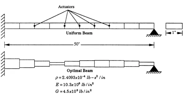
Belvin and Park [4] work out an example on an idealized beam (Figure 1.1). The beam is cantilevered at the root and pinned at the tip. The beam consists of ten Timoshenko beam elements of equal length and width. The design parameters in this problem are the thicknesses of the elements. There are five transverse force actuators located at the positions shown in the figure, and the control is full state feedback.

(28)

Actuators

Uniform Beam

1"

1-

5011-p z.IUkwxivU 0o-8s /tin

E= 10.3x106

lb/in2 G = 4.5x106 lb/in2

Figure 1.1: Cantilevered-Pinned Beam used by Belvin and Park

The disturbance is an initial velocity and displacement error corresponding to the peak response due to a step force given by:

f

= M1/2T- (1.29)

where T is the mass normalized modal transformation matrix and - is an arbitrarily selected vector of ones. Thus, the disturbance force effects all modes of the system equally.

The design goal is to minimize the quadratic cost:

j=

O

XQ

+

UTRu)

dt

(1.30)

with the state and control penalty matrices selected to penalize the system energy and static control work.

Q=

-K

0 R = FTK-1F

(1.31)

0 7÷M

where F is the control input matrix. The constants y, and -y are arbitrary in this problem. The mass of the system is held fixed, and all of the element thicknesses are allowed to vary under the constraint that they remain above a small, non-zero, minimum value.

(29)

The lower part of Figure 1.1 shows the optimum design found for this problem which was found to be independent of -y, and y,:. The distribution of material is strikingly similar to what one would expect the bending strain distribution to be for the first mode of the uniform beam. Belvin and Park were actually able to prove that for this problem formulation, the cost is inversely proportional to the cube of the natural frequency of the first mode when the number of actuators is equal to the number of modes retained in the design model. Clearly, this inverse cube relationship prefers stiffening of the first mode over all other mechanisms for improving controlled performance. This type of answer is very encouraging. One would like to have the cost associated with a mode of the structure go down as the frequency of the mode goes up. This will allow one to truncate the plant model with good confidence because the higher frequency modes will not participate very strongly in the cost.

In Table 1.2, there were two approaches which could involve the technique of stiff-ening the system. The first is to stiffen the system against the disturbance. In their work, Belvin and Park show that the peak response used as the initial condition was inversely proportional to the stiffness of the system. This means that the influence of the disturbance in the cost in inversely proportional to the fourth power of the frequency. It is clear from this that the the stiffening in this example is, in fact, needed to reduce the disturbability.

1.2.2 Example 2: Truss example of Miller and Shim

A truss example appears in the work done by Miller and Shim [6]. Their structure is a ten bar, two-dimensional truss (Figure 1.2). The truss members are modelled as bar elements with pinned joints, and the design variables are their cross-sectional areas. There are lumped masses located at each node. These masses are fixed and are large enough that the mass of the rest of the structure can be ignored in the dynamic response. There are four actuators, one at each free node, capable of exerting vertical forces. The control is full state feedback.

(30)

E= 107 p= 2.588x10-4 Lumped Masses at nodes 1.29 kg vesign v arinaes: Areas of Members

Figure 1.2: Ten bar truss used by Miller and Shim

The objective of the control and structural design is to minimize the cost:

J = q₁W

+

q2

j0

(xTQx + UTRu) dt (1.32)

where W is the weight of the structure, and the state and control penalty matrices penalize system energy and static control work.

0

M

The weighting parameters ql and q2 were selected to achieve a "sufficient" reduction in the dynamic performance cost and weight in the structure from a nominal, uniform structure.

The initial conditions for this problem correspond to the static deflection of the truss due to a prescribed loading which was instantaneously removed. Two cases were examined. In the first case, the loading was an equal upward force at each free node of the truss. In the second case, the loading was again equal forces at each node, but the loading at the inner two nodes was downward and not upward. The first loading was selected to excite primarily the first mode of the structure, while the second was selected to excite the second mode.

The free structural parameters in this problem are the cross sectional areas of the members. Figures 1.3 and 1.4 show the optimal cross sectional areas obtained by Miller

(31)

AT-!.:

-1

Static Load: Upward force at

all four nodes

Figure 1.3: Optimal design for load case 1

I Static load: Upward on outboard nodes, Downward on inboard nodes 2 2

Figure 1.4: Optimal design for load case 2

and Shim for the two static load cases. Notice that in their optimal design for the second load case, there is a significant amount of material in the battens (members 2 and 5). Because these would normally be low stain areas for the problem described, it was decided to redo the optimizations for both load cases. The results obtained by this author are compared to those of Miller and Shim in Figures 1.5 and 1.6. There is close agreement between the designs obtained by Miller and Shim and those obtained here for the first load case. In the second design, it was found that the cross sectional areas of the battens went to the minimum side constraints. Miller and Shim reported that they were having difficulty with the penalty functions used to meet the constraints. Most likely, this was the source of the discrepancy.

(32)

Design Number 1

Optimal Design of Miller and Shim E Strain due to static load Optimal design of author E Strain due to first mode

1,3 2 4,6 5 7,8 9,10

Member number

Optimal designs of Miller and Shim and this author for due to static load and first mode.

first load case, and strain

Optimal design Optimal design

Design Number 2 of Miller and Shim El of author 1"

Strain due to static load Strain due to second mode

1.5

0

1,3 2 4,6 5 7,8 9,10

Member number

Optimal designs of Miller and Shim and this author for second strain due to static load and second mode.

load case, and

0.8 0.6 0.4 0.2 0 Figure 1.5: Figure 1.6: r 1 i i i i 1

(33)

Although Miller and Shim do not go into it, there is a very interesting explanation for why the designs obtained are optimal. Because of the size of the lumped masses at the nodes, increasing member size does very little to change the mass matrix, hence the purpose of added material in this problem is to stiffen the system. As mentioned above, one might stiffen the system to speed up the open loop dynamics or reduce the sensitivity of the system to the disturbance forces. Included in Figures 1.5 and 1.6 are the strains induced in the members of a uniform structure due to the static loadings and also due the the first and second mode shapes. Remember, the first load case was selected by Miller and Shim to excite the first mode, while the second was selected to excite the second mode.

Comparison of the first optimal design with the static and modal strains is incon-clusive. There is good agreement for all three. In the second case, the modal strain is much larger than the static strain in members 9 and 10 and smaller in members 4 and 6. The optimal design, however, agrees very closely with the static strain, hence one can be reasonably certain that the goal of stiffening the system is solely an attempt at reducing the influence of the disturbance.

1.2.3 Example 3: Beam example of Onoda and Haftka

Onoda and Haftka [23-26] use a beam-like structure to demonstrate their optimization algorithm. The upper part of Figure 1.7 shows a depiction of their structure. The disturbance is assumed to be a stochastic force acting along the entire length of the structure:

p(x, t) = /3(x/L)f,(t) -L < x < L (1.34) where f,(t) is Gaussian White Noise. Because this disturbance is asymmetric and it is correlated over the entire length of the structure, only the asymmetric modes of this symmetric structure need to be considered. A Bernoulli-Euler beam consisting of five finite elements used in their analysis is shown in the lower part of the figure.

(34)

Actuators

x = -Xc X = Xc

Figure 1.7: Beam-like spacecraft of Onoda and Haftka

Two types of controllers were used-direct output feedback and full state feedback. However, attention here will be restricted to the full state feedback case as the output feedback case did not produce any designs significantly different from the full state feedback case.

The design variables were the cross-sectional areas of the finite elements and the position of a torque actuator. The stiffness and mass of each element is assumed to be proportional to its area.

The design objective in this case was to minimize a weighted sum of the the mass of the structure and the control effort:

J

=

qi W + q2 u2dt (1.35)

The weighting parameters qi and q2 were selected according to assumptions regarding the mass of the controller as a function of the control effort.

The performance of the system was constrained:

jP

=

f

XTqxdt

<• J

(1.36)

The matrix Q was selected to penalize the mean square displacement along the beam:

xTQx - y'dx (1.37)

where y is the vertical displacement of the beam as a function of the spatial coordinate

(35)

Large upper bound on displacement Small upper bound on displacement

Figure 1.8: Optimal designs for Haftka and Onoda's beam problem.

Figure 1.8 shows the two types of optimal designs found by Onoda and Haftka. The first one corresponds to the case when Ju had a modest value (Expensive control). The similarity between this shape and the strain distribution for the first mode of this system makes it clear that the objective is simply to stiffen the first mode. The shape of the disturbance is identical to the mode shape for the rigid body mode and hence, it will be orthogonal to the other modes. Hence, the stiffening of the first mode is not meant to reduce the influence of the external disturbance. Instead however, it appears that its purpose is to keep the actuator from disturbing this mode as it attempts to correct the error induced in the first mode. As JIA is made smaller (tighter constraint on controlled performance) the shape approaches the second one shown in the figure. Onoda and Haftka suggest that placing mass at the end is an attempt to reduce the disturbability of the system, as this is where the disturbance is largest. This surmise is most likely correct, as the system has little strain at that point, and therefore, it cannot be there for stiffening.

1.2.4 Example 4: Compression rod example of Messac et. al.

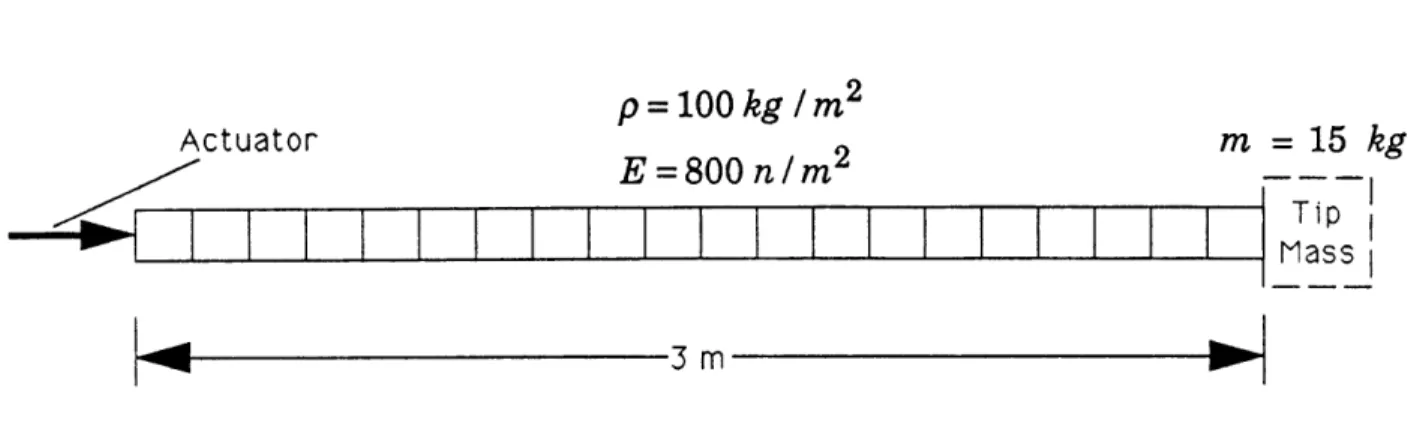
Messac, Truner, and Soosaar [11] use a finite element rod (Figure 1.9) as an example of controlled structure optimization where the disturbance is a slew maneuver. The rod is composed of twenty rod finite elements of equal length. The structural design variables are the cross-sectional areas of the elements. In one case, an extra lumped mass was included at the right end of the rod. In the other case, this mass was omitted.

The actuator in this problem is a force actuator at the left end of the rod which acts along the rod's axis. The goal is to translate the rod from an initial rigid body

(36)

p = 100 kg / m2

Actuator 2 _{m = 15 kg}

E= 800 n / m2

-Tip I

Mass

Figure 1.9: Compression rod of Messac et.al.

displacement, to a final displacement of zero. The cost for this problem was:

J = x SX + tf (QX

+ U2)

dt (1.38)

where xf is the state vector at time t = tf and the matrices

Q

and S are selected to penalize the sum of the squares of the nodal displacements. Also, S was selected to be approximately nine orders of magnitude larger than Q to ensure that the final error was very small.

The control u(t) is always optimal. Note that because the cost functional is over a finite time, the control cannot be expressed as a time-invariant gain matrix multiplying the state. However, optimal control theory does make it possible to compute the control and evaluate the cost for any reasonable vector of structural parameters.

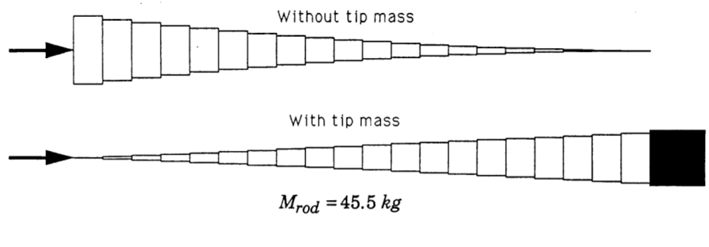
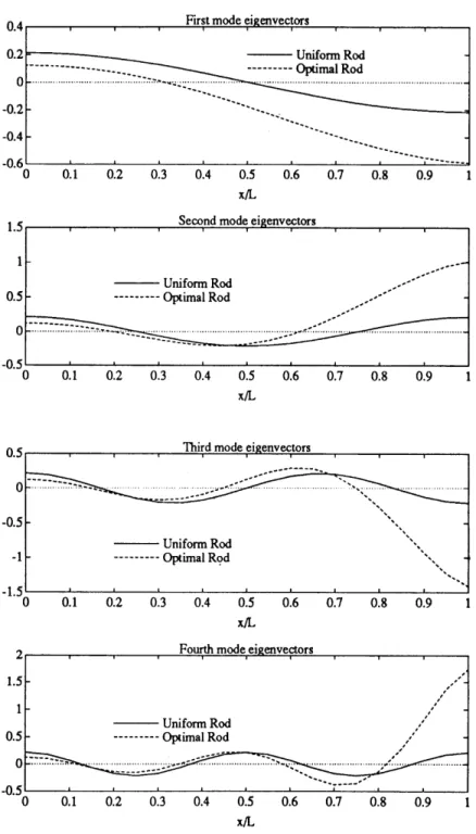
The structural design parameters in this problem were the cross sectional areas of the finite elements, and the total mass of the structure was held constant. Two different designs were obtained without and with the tip mass (Figure 1.10). In both, the first modal frequency was substantially increased. However, the two designs seem to be mirror images of each other. Messac et al provide a good explanation for the optimal design without the tip mass. Figure 1.11 shows the displacement eigenvectors for the optimal bar and a uniform bar of equal mass. The displacement in the first four flexible modes at the actuator has been substantially decreased. In this slew maneuver, the initial displacement is all in the rigid body mode. The flexible modes are initially undisturbed.

(37)

Without tip mass

With tiD mass

Mrod = 45.5 kg

Figure 1.10: Optimal designs for compression rod

As the controller acts to correct this, it will cause disturbances in the other modes which will have to be controlled out. Reducing the displacement in the first four flexible modes at the actuator will reduce this. Messac et al point out that it is this type of improvement that eigenvalue optimization will miss.

This same argument can be applied to the case with the tip mass to show that the goal is to make the flexible modes more controllable.

1.2.5 Example 5: Cantilevered beam example of Milman et.

al.

Milman, Salama, Scheid, Bruna, and Gibson use several examples to illustrated their ho-motopy algorithm. The first consists of a cantilevered beam composed of three Bernoulli-Euler finite elements (Figure 1.12). Each element has a circular cross section, and the structural variables are the cross-sectional area of each element. The control is full state feedback acting through a transverse force actuator located at the tip of the beam. The disturbance acting on the system is a pressure wave modelled as three uncorrelated force impulses located at the free nodes of the beam.

The design goal is to find a combination of structural parameters which will optimize a composite cost function based on the structural mass and the performance of the

(38)

First mode eieenvectors

0 0.1 0.2 0.3 0.4 0.5 0.6 0.7 0.8 0.9

Second mode eigenvectors

0 0.1 0.2 0.3 0.4 0.5 0.6 0.7 0.8 0.9

Third mode eigenvectors

0 0.1 0.2 0.3 0.4 0.5 0.6 0.7 0.8 0.9

Fourth mode eigenvectors

0 0.1 0.2 0.3 0.4 0.5 0.6 0.7 0.8 0.9

Figure 1.11: Eigenvectors and eigenvalues for the uniform and optimal compression rods (no tip mass).

0.5 S --- Optimal RodUniform Rod

I i i i | i i i

---

----Uniform Rod --- Optimal Rod --- Uniform Rod --- Optimal Rod --- I I I . q. Uniform Rod

---

--- Optimal

Rod

..

.

..

.

..

.

..

.

... ...

I r 1 . .. I ! I ... wll " 1 -1 51 0.5

(39)

Pressure Impulses p= 1660 kg /m3 E= 9.56x1010 n/ m2

Ihub = 50 kg m

2

45

f

Actuator

Figure 1.12: Cantilevered beam of Milman et.al system when LQR control is used:

JA = (1

-

A)J

+J

3

J, = - pliA1

i=1

Jc = (rTQ,r + +TQ,ý + uTRu)dt (1.39)

where li, Aj, and p are the length, cross-sectional area and density of element i, and r, r, and u are the displacement, velocity, and control vectors for the system.

The matrices Q, and Q, are arbitrarily defined to be 100K, and 100M respectively, where M and K are the mass and stiffness matrices of the system. This type of state weighting penalizes the total energy in the system. The matrix, R, weights the control effort and is defined to be 10- 4.

The parameter, A, was varied form zero to unity and the composite cost, JA, was optimized at each point. This generates the family of designs which represent optimal trade-offs between performance and mass.

The same basic shape was obtained for all values of A. The top half of Figure 1.13 depicts the optimal design for the structure with a mass of 466 kg (A = .99). Milman et. al. reason that the control force at the tip of the beam makes the closed loop modes similar to those of a cantilevered-pinned beam. The similarity between their optimal design and the first strain mode shape of a cantilevered-pinned beam leads them to

An approach to the preliminary design of controlled structures

An Approach to the Preliminary Design of

Controlled Structures

Robert Normand Jacques

©

FEB 19 1991

An Approach to the Preliminary Design of Controlled Structures

Acknowledgements

Contents

Chapter 1

Introduction to Controlled

Structure Optimization

1.1

Literature Review

(0

I

r(t)

0

0

1F(t)

-M-1K

-M-1D

i

M-1F

v(t)

(t)

(1.2)

~k1'=

(1.5)

Act

1.1.1

Problem Formulations

a<

< a .i

_a<

(1.8)

>

J,

=

Q j o

xj

+

(

'

(t)Q(t) + uT(t)Ru(t))

dt

(1.17)

J

=

lim E [T(t)Qt)

+

uT(t)R~(t)]

(1.19)

j

=

J3 = -(CC1

(1.25)

ff

J =

xQX

(Ru)

+

dt

(1.26)

1.1.2

Solution Methods

1.1.3

Result Analysis

1.2

The Approaches to Improved Performance

modelled modes

1.2.1

Example 1: Cantilevered beam of Belvin and Park

Uniform Beam

1"

1-

f

j=

O

XQ

_(1.26)