HAL Id: hal-02745873
https://hal.inrae.fr/hal-02745873
Submitted on 3 Jun 2020
HAL is a multi-disciplinary open access
archive for the deposit and dissemination of
sci-entific research documents, whether they are
pub-lished or not. The documents may come from
teaching and research institutions in France or
abroad, or from public or private research centers.
L’archive ouverte pluridisciplinaire HAL, est
destinée au dépôt et à la diffusion de documents
scientifiques de niveau recherche, publiés ou non,
émanant des établissements d’enseignement et de
recherche français ou étrangers, des laboratoires
publics ou privés.
Observations in DEVS framework
Gauthier Quesnel, Ronan Trépos, Patrick Chabrier, Jennifer Baudet, Raphaël
Duboz
To cite this version:
Gauthier Quesnel, Ronan Trépos, Patrick Chabrier, Jennifer Baudet, Raphaël Duboz.
Observa-tions in DEVS framework. Symposium on Theory of Modeling and Simulation (DEVS/TMS 2011),
Labo/service de l’auteur, Ville service, Pays service., Apr 2011, Boston, United States. �hal-02745873�
Observations in DEVS framework
Gauthier Quesnel1, Ronan Tr´epos1, Patrick Chabrier1, Jennifer Baudet1, Rapha¨el Duboz2and ´Eric Ramat3
1INRA, UR875 Biom´etrie et Intelligence Artificielle 2ULCO, LISIC 3Cirad, Gestion Integr´ee des Risques
F-31326 Castanet-Tolosan, France 50 rue Ferdinand Buisson BP 719 Campus de Baillarguet
62228 Calais Cedex, France 34398 Montpellier cedex 5, France
[email protected] [email protected] [email protected]
Keywords: DEVS, observation, methodology and simula-tion.
Abstract
The observation of a model is a necessary process in the con-text of modeling and simulation as it offers to modelers the results of their simulations. In this paper, we focus our works on the observation mechanism which is generally not explicit nor clearly specified. This is generally not an issue unless we want to use our model in experimental frames or to avoid the observation mechanism to interfere with the simulation. In this paper, we introduce an extension to the Parallel Discrete
Event System Specification(PDEVS) formalism, to observe
models in various ways, by event (at each state transition of a model), at the end of the simulation or by a time step. Thus, we define a formal specification of this extension and its abstract simulators algorithms. Finally, we present an im-plementation in the DEVS framework VLE.
1.
INTRODUCTION
In the Modeling and Simulation (M&S) activity, observa-tion of the behavior of models is a major task. Observaobserva-tion is the process that catches the state of a model during or at the end of the simulation. It allows the modeler to test, prove, validate or generate data from simulations by connecting sim-ulation software to output streams like files, databases, unit test or visualisation softwares for instance. Observations con-tribute to the modeller’s representation of its studied system. Nevertheless, the observation processes are generally not ex-plicit nor specified in formalism or in simulation software. Thus, they are often model dependant and they simply con-sist in source code extension. However, on the major M&S software, observations are integrated in the simulation model like in Ptolemy II [7] or in Modelica [11].
This is generally not useful to specify formally the observa-tion process. However, it becomes necessary when we want the observation to be modeled as a part of an experimental frame [13, 12, 1], where simulation results have to be cap-tured following a precise experimental plan. For instance, in experimental frame, to calibrate a model or to make a sensi-tivity analysis, only a final observation of the system is nec-essary but in online optimisation by simulation or generally
in dynamical experimental frames, we need the trajectories of variables of the models [5].
Our works take place in the M&S theory defined by B. P. Zeigler [13]. M&S theory tends to be as general as pos-sible. It addresses major issues of computer sciences from ar-tificial intelligence to model design and distributed simula-tions. M&S theory aims to develop a common framework, formal and operational, for the specification of dynamical systems. In this paper, we consider the Discrete Event
Spec-ification System(DEVS) formalism [13] from B. P. Zeigler
works to develop a formal observation for the M&S theory. The DEVS formalism is well situated to clearly specify both system dynamics and experimental frames [13, 12]. Never-theless, even if it is possible to specify observations using DEVS without any modification, it appears that the addition of a specific function dedicated to observation process can be very useful and computationally more efficient than a classic DEVS implementation (cf. figure 1). In this paper, we pose to extend the DEVS formalism with an observation pro-cess. These changes allow the modeler to observe its models in different ways.
2.
METHOD
Before proposing the formalisation of the extension ob-servation, we briefly describe, in the following section, the PDEVS formalism.
2.1.
PDEVS
DEVS [13] is a well-known and accepted formalism for the specification of complex discrete or continuous systems abstracted as a network of concurrent, timed and interacting atomic and coupled models. PDEVS [3] extends the Classic DEVS [13] essentially by allowing bags of inputs to the exter-nal transition function. Bags can collect inputs which are built at the same date, and process their effects in future bags. This formalism offers a solution to manage simultaneous events that could not be easily managed with Classic DEVS. For a detailed description, we encourage the reader to read the chapter three in [13].
PDEVS defines an atomic model as a set of input and out-put ports and a set of state transition functions:
M= hX ,Y, S, δint, δext, δcon, λ, tai Where:
Xis the set of input values
Y is the set of output values
Sis the set of sequential states
ta: S → R+0 is the time advance function
Q= {(s, e)|s ∈ S, 0 ≤ e ≤ ta(s)}
Qis the set of total states,
eis the time elapsed since last transition δint: S → S is the internal transition function δext: Q × Xb→ S is the external transition function
Xbis a set of bags over elements in X
δcon: S × Xb→ S is the confluent transition function, subject to δcon(s, /0) = δint(s)
λ : S → Y is the output function
If no external event occurs, the system will stay in state s for ta(s) time. When e = ta(s), the system changes to the state
δint. If an external event, of value x, occurs when the system
is in the state (s, e), the system changes its state by calling
δext(s, e, x). If it occurs when e = ta(s), the system changes
its state by calling δcon(s, x). The default confluent function δcondefinition is:
δcon(s, x) = δext(δint(s), 0, x) The modeler can prefer the opposite order:
δcon(s, x) = δint(δext(s,ta(s), x))
Of course, this function can be completely defined by the modeler.
Every atomic model can be coupled with one or several other atomic models to build a coupled model. This operation can be repeated to form a hierarchy of coupled models. The set of atomic and coupled models and their connections is named the structure of the model. A coupled model is defined by:
N= hX ,Y, D, {Md}, {Id}, {Zi,d}i
Where X and Y are input and output ports, D the set of models and:
∀d ∈ D, Mdis a PDEVS model
∀d ∈ D ∪ {N}, Idis the influencer set of d : Id⊆ D ∪ {N}, d /∈ Id
∀d ∈ D ∪ {N},
∀i ∈ Id, Zi,dis a function, the i-to-d output translation: Zi,d: X → Xd, if i = N
Zi,d: Yi→ Y, if d = N
Zi,d: Yi→ Xd, if i 6= N and d 6= N
The influencer set of d is the set of models that interact with
d and Zi,d specifies the types of relations between models i
and d.
In previous section, we present succinctly the PDEVS for-malism. In the following paragraphs and sections, we propose the formalization and abstract simulators of our observation extension.
2.2.
Formal specification
The construction of a DEVS platform for modeling and simulation (like presented in section 3.) implies to observe models and their evolution during the simulation. Observa-tion of DEVS models involves watching or capturing their states. These captures can be done when a change of state occurs (in DEVS terminology, in δint, δext or δcon transition functions) or at specific dates.
Observation of models is a necessary process in the context of the modeling and simulation. To develop a useful simulator software based on DEVS or which accepts DEVS models and theirs computation like OSA [10] or James II [6], for the mod-ellers, the observation can be separated from the models be-haviour. OSA or James II use classical software engineering paradigm to develop observation. Respectively “aspect ori-ented” techniques for OSA or the “design pattern observer” in James II. In this paper, we consider the development of the observation mechanism into the DEVS formalism itself. This work allows to clearly and formally defines when and how to observe models in a “all DEVS” vision of the simulation.
In DEVS, the commonly used solution (as presented in fig-ure 1), is to connect models, both inputs and outputs, to an observation model. This model has in charge to send obser-vation messages and to process the responses of the models. For instance, to build a discrete observation, the observation model relies on a constant ta function in order to send, at each time step, an event to observed models. Then, observed mod-els output observation values that are sent to the observer.
This solution forces the modelers to merge the state graphs between observation and behavior of their models (See figure 2 for an explanation). In addition, by merging the state graphs, the modeler may make the results of its models dependent to the observation he makes. For example, if a model is ob-served asynchronously with its behaviour, the computation of the e or internal state variables, can give different results with or without observations. Precisely, this mismatch can be explained by the difficulty in representing reals in computer engineering [4] (see the IEEE Standard for Floating-Point Arithmetic, IEEE 754) .
Finally, in DEVS, a model can have several states at the same date (when at least one call to the ta(s) function returns 0). These states are known as transitory states. It seems ob-vious that the observation of the transitory states makes no sense. However, this solution does not guarantee to provide
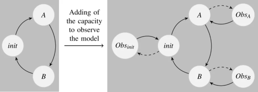
init A B init A B Obsinit ObsA ObsB Adding of the capacity to observe the model
Figure 2. These pictures show state graphs of an atomic model. In left picture, we show the model without observation and in the right part, the same model with the capacity to be observed at any time (dotted lines represent external transitions). In the computation of the observation states Obsinit, ObsAor ObsB(in δext, δint, δconf or ta functions), simulators can introduce floating-point errors when computing the time elapsed since last transition (e in DEVS terminology) for example.
Figure 1. This picture shows the classic observation mech-anism to observe models in the DEVS formalism. Three atomic models A, B and C are observed by an observation model O which sends event for request observation on output Yobsand waits the results on input port Xobsin order to store it in output files, databases etc.
only observations of real model states. For example, if the observation is required at a specific time of simulation, the state observed can be one of these transitory states.
In this section, we propose a formal and operational repre-sentation of observations in the PDEVS formalism. This ex-tension is based on a function of observation in atomic models and a second graph of connections in coupled models. This extension to the PDEVS formalism integrates necessary char-acteristics:
• first is to ensure that this extension does not disturb the simulation i.e. we need to conserve the same result with or without the observation.
• second is to provide several types of observation. We propose, in this paper, two modes: time step and finish which define respectively: observations when a model
reaches a time and observations at the end of the simu-lation. (See figure 3).
• finally, in DEVS, a model may change several times statements to the same date (when its ta returns 0 or an external events disturb it). In this case, we observe the last state of the model.
Thus, to develop this extension we need to add function to the atomic models, to add new set in coupled model and add specific observation models. We develop these changes in the next section.
2.2.1. PDEVS Atomic model
To develop this extension in the PDEVS formalism, we ex-tend the PDEVS atomic model with new sets of input and out-put ports (Xobs?and Yobs). The first one is used for observation request, the second one is used for routing values returned by modeler. We attach to this port a new output function called
λobs. The new PDEVS atomic model is defined such as:
M= hX ,Y, S, Xobs?,Yobs, δint, δext, δcon, λ, λobs, tai Where:
Xobs?are the ports used to catch observation requests
Yobsare the ports used to send observation values
λobs: Xobs?× s × tobs→ Yobs s∈ S,
tobscurrent time of the simulation.
This definition allows us to represent both observed mod-els and classical PDEVS modmod-els as defined in section 2.1.. Indeed the model hX ,Y, S, Xobs?,Yobs, δint, δext, δcon, λ, λobs, tai
with no observations1is equivalent to the classical PDEVS
1X
t S State of a model t S Finish observation t S Timed observation t S Event observation Figure 3. This figure shows three modes for observing the state of a system (in the top chart). In the next charts, we use an arrow to show when an observation occur. Thus, in the second chart, we show a finish observation at the end of the simulation, in the third chart, we show a time step observation
with a duration of ∆t= 0.5 between two observations and
fi-nally, we show an event view, when the value of the observed variable crosses thresholds.
atomic model hX ,Y, S, δint, δext, δcon, λ, tai. In fact, we should distinguish observed models from observer models.
2.2.2. Observer models
In this paper, we suggest two types of observers. Otimed,
and Ofinishto respectively, send observation following a given
time-step or at the end of the simulation.
• The discrete time observer model, Otimed, needs to send
output events on its output port Yobsevery ∆t unit time.
Otimed reads observation events from its port Xobs and
stores data transported by event. This model is :
Otimed= hXobs,Yobs?, S, Xobs?,Yobs, δint, δext, δcon, λ, λobs, tai
Where:
Xobsis the set of observation values, Yobs?is the set of observation requests,
S: {IDLE, SENT} × Data, with:
IDLE, SENT: automata finite states,
Data: output stream states (files, database, etc.). Xobs?= /0
Yobs= /0
∀d ∈ Data : δint((IDLE, d)) = (SENT, d)
∀d ∈ Data : δint((SENT, d)) = (IDLE, d)
∀s ∈ {IDLE, SENT } : δext((s, d), e, Xobs) = (s, d0)
where d0is the state of the output stream once
Xobshas been stored,
∀d ∈ Data : ta((IDLE, d)) = ∆t (the time step)
∀d ∈ Data : ta((SENT, d)) = 0 ∀s ∈ S : λ(s) = build request(s) λobsis a null function
• The finish observer model, Ofinish, produces observation
events at the end of the simulation on it Yobs port and
wait observation events from its port Xobs. Ofinishis the
same model as Otimedbut, its ta function returns the end
of the simulation to build observation event, or +∞ after. Otimed= hXobs,Yobs?, S, Xobs?,Yobs, δint, δext, δcon, λ, λobs, tai
Where:
Xobsis the set of observation values, Yobs?is the set of observation requests,
S: {WAIT, END} × Data, with:
WAIT, END: automata finite states,
Data: output stream states (files, database, etc.).
∀d ∈ Data : δint((WAIT, d)) = (END, d)
∀d ∈ Data : δint((END, d)) = (END, d)
∀s ∈ {WAIT, END} : δext((s, d), e, Xobs) = (s, d0)
where d0is the state of the output stream once
Xobshas been stored,
Xobs?= /0 Yobs= /0
∀d ∈ Data : ta((WAIT, d)) = end
where end is the duration of simulation ∀d ∈ Data : ta((END, d)) = +∞
∀s ∈ S : λ(s) = build request(s) λobsis a null function
The function build request is a user defined function that
identifies in Yobs?the observation request that should be sent
to the observed models.
2.2.3. Coupled model
As seen earlier in the introduction and in the section 2.1.,
the Idvariable and the function Zi,d define the graph of
con-nections of the models by calculating the influencees mod-els. Our observation extension of the PDEVS formalism uses
the same principle. It proposes two subsets Ioand Ir which, respectively identify the influencees of atomic models (re-sponses of the observations) and the influencees of observer models (models sending the request of observation).
We extend the PDEVS model coupled in order to introduce a second connection network (see the figure 4). This second network is dedicated to the observer models and to the clas-sical PDEVS atomic models to observe through their ports
Xobs?and Yobs. The new PDEVS coupled model is defined as:
N= hX ,Y, D, O, R, Xobs?, Xobs,Yobs?,Yobs, {Md}, {Id}, {Zi,d},
{Mo}, {Od}, {Zo,d}, {Mr}, {Rd}, {Zr,d}i Where Xobs, Yobsand Xobs?, Yobs?are input and output ports to route observation and request events. O is the set of names
of observed models O ⊆ D, {Mo} is the set of observed
mod-els {Mo} ⊆ {Md} , R is the set of names of observer models
R⊆ D and {Mr} is the set of observer models {Mr} ⊆ {Md}.
∀r ∈ R ∪ {N},
Iris the influencer set of observed models of r : Ir⊆ O ∪ {N}, r /∈ Ir
∀o ∈ O ∪ {N},
Iois the influencer set of observed models of o : Io⊆ R ∪ {N}, o /∈ Io
The observation network is however very constrained.
Thus, the functions Zo,dand Zr,d are very different and
pro-vide additional constraints from the classical Zi,d function.
These additional constraints ensure that a DEVS atomic model cannot send an observation event to another DEVS atomic model, and an observation model cannot send request observation to another observation model. The figure 4 shows an example of connections between observed and observer models.
∀r ∈ R ∪ {N},
∀d ∈ Ir, ∃ an output translation function Zr,d: Zr,d: Xobs?→ Xobs?d, if r = N
Zr,d: Yobs?r → Yobs?, if d = N
Zr,d: Yobs?r → Xobs?d, if r 6= N and d 6= N
∀o ∈ O ∪ {N},
∀d ∈ Io, ∃ an output translation function Zo,d: Zo,d: Xobs→ Xobsd, if o = N
Zo,d: Yobso → Yobs, if d = N
Zo,d: Yobso → Xobsd, if o 6= N and d 6= N
Closure under coupling
As we do not change the internal S of coupled or atomic models nor all sets of the PDEVS definition (IMM, INF(s),
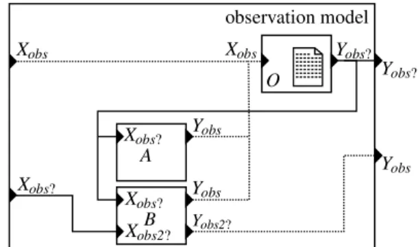
Figure 4. In this picture, we illustrate the second network in the coupled model to deal with observations graph. Plain
connections are observation requests from output port Yobs?
of observation models, to atomic model input port Xobs?or to
coupled model’s output port Yobs?, or from coupled model
in-put port Xobs?to atomic model Xobs?. Dashed connections
con-stitute response of observation request from extended PDEVS
atomic model (on output port Yobs) to observation model Xobs
or coupled model output port Yobs. The atomic model B is
ob-served by an external observation model on its port Xobs2. It
sends observations to its output port Yobs2. For this figure and for a better understanding, we distinguish observation ports for the model B.
CONF(s), EXT(s) and UN(s) of the coupled model), the PDEVS functions have the same content (See chapter 7 in [13] to the complete formalization), and the closure under coupling property of the extension observation for parallel DEVS is still verified.
2.3.
Algorithms
2.3.1. Root coordinator
The root-coordinator implements the overall simulation loop. It sends messages to its direct subordinate (simulator or coordinator). The root-coordinator first sends an initial-ize message (i-message), and loop on internal transition (*-message) from its child to perform the simulation cycles until some termination conditions.
1 Parallel−Devs−Root−Coordinator 2 variables:
3 t // current simulation time
4 child // direct subordinate devs−simulator or devs−coordinator 5
6 t= t0
7 send initialization message (i,t) to child 8 t= tn of its child
9 loop
10 send (∗,t) message to child 11 t= tn of its child 12 until end of simulation
As describe in previous algorithm, the root coordinator is not modified in this extension.
2.3.2. Coordinator
In the coordinator algorithm, we add an additional variable
tbwhich indicates the last date of the simulation. This
vari-able tb detects the last PDEVS bags to ensure to observe the latest state of a model. We add a new bag, called mailobs to store all observation events to atomic models at a specific date. When tb detect a change, the mailobs is flushed into the
observation network using the functions Zr,dand Zo,d.
1 Parallel−Devs−Coordinator 2 variables:
3 DEVN= (X , Y , D, {Md}, {Id}, {Zi,d})
4 parent // parent coordinator 5 tl // time of last event 6 tn // time of next event
7 eventlist // list of element (d, tnd) sorted by tnd
8 mail // output mail bag
9 mailobs // observation mail bag
10 Oevent// event−list of event observation model
11 yparent// output message bag to parent
12 yd// set of output message bags for each child d
13
14 when receive xobs−message (xobs,t)
15 if not (tl ≤ t ≤ tn) then
16 error: bad synchronisation
17 receivers = {o|o ∈ children, o ∈ Ir}
18 for each o ∈ receivers
19 send x−message (Zr,d(x) with input value Zr,dto o
20
21 when receive xobs?−message (xobs?,t)
22 if not (tl ≤ t ≤ tn) then
23 error: bad synchronisation
24 receivers = {r|r ∈ children, r ∈ Io}
25 for each r ∈ receivers 26 add r, xobs?to mailobs
27
28 when receive yobs−message (yobs,t) from o
29 for each child d ∈ Zo,d
30 send xobs−message to d
31 for each d ∈ Zo,dand d = N
32 send yobs−message to parent
33
34 when receive yobs?−message (yobs?,t) from r
35 for each child d ∈ Zr,d
36 send yobs−message to d
37 for each d ∈ Zr,dand d = N
38 send yobs?−message to parent
39
40 // finally, we append these algorithms in the following message 41
42 when receive i−message (i,t) at time t 43 [...] // The same algorithms than PDEVS 44 tb= tl
45
46 when receive ∗−message, x−message or y−message 47 if tb != t then
48 for each r, xobs?∈ mailobs
49 send xobs?−message (Zr,tb(x) with input value Zr,dto r
50 mailobs= /0
51 tb= t
52 [...] // The same algorithms than PDEVS 53
54 end Parallel−Devs−Coordinator
• from l. 1 to l. 38: routes the message or stores in mailobs. • from l. 40 to the end: to update the tb variable and to
send xobs?-message to the atomic models.
2.3.3. Simulator
Lastly, this last section on the abstract simulators devel-ops algorithm for the simulator of the atomic model. As pre-sented previously, the management of the observations events is very simple for the modeler since only one function is
called λobs. This function is called only for classical atomic
models when they receive an Xobs?event. When observation
models receives Xobs event, they use the classical way when
receiving input message (See x-message in PDEVS abstract simulators).
1 Parallel−Devs−Simulator 2 variables:
3 parent // parent coordinator 4 tl // time of last event 5 tn // time of next event
6 DEV S // associated model with total state (s,e)
7 yobs// output observation bag
8
9 [...] // The same algorithms than PDEVS simulator see chapter 11. 10
11 when receive xobs?−message (xobs?,t) at t with input xobs?
12 yobs= λobs(xobs?,t)
13 send yobs−message (yobs,t) to parent coordinator
14
15 end Parallel−Devs−Simulator
• l. 12: when receives an xobs?-message from the parent,
simulator computes the observation in the λobsfunction
and sends the data (wrapped into an yobs-message) to the parent coordinator.
To validate this work, these abstract simulators are imple-mented in VLE, a platform of modeling and simulation VLE.
3.
RESULT
Our works have started with multi-disciplinary issues emerging from the interaction between computer scientists and biologists. Considering these works, we think that the integration of heterogeneous models and the respect of the M&S cycle are the key issues to provide a complete and reliable software environment for natural complex systems modelling. So, VLE (Virtual Laboratory Environment) has evolved toward a complete multi-modelling and simulation environment [8] and is now a generic environment for M&S, in Environmental Sciences, in Industry or Medicine. It is used
in many projects from two major French research institutes INRA and Cirad like the RECORD project [2]. RECORD is a platform designed for developing models of cropping sys-tems, including crops, soils, pests, pathogens, and farmers, at different spatial and temporal scales. Scientists will use the RECORD platform to develop new models as modular com-ponents, to re-use and combine them in order to represent cropping systems and to share them with the community.
Technically, VLE is a set of softwares and libraries which supports multi-modeling and simulation by implementing the PDEVS abstract simulators and a DEVS bus. VLE is ori-ented toward the integration of heterogeneous formalisms like integration of ordinary differential equations (DESS, QSS 1 and 2), petri nets, finite state automata (moore, mealy, UML statechart), cellular automata (Cell-DEVS and Cell-QSS) and agent. Furthermore, VLE is able to integrate specific models developed in most popular programming languages into one single multi-model. Finally, VLE uses an open-source license and all the source code are available on its website including this observation extension (see the figure 5 for screenshots of VLE).
3.1.
Implementation
In our implementation of the PDEVS abstract simulator, we define an atomic model as a classical C++ class. This class must be inherited to override the observation function and to benefit to the observation extension developed in the previous section.
1 class Dynamics { 2 public:
3 Time timeAdvance() const;
4 void internalTransition(const Time& time);
5 void externalTransition(const Time& time, const ExternalEventList& lst); 6 void output(const Time& time, ExternalEventList& out) const;
7 void confluentTransition(const Time& time, const ExternalEventList& lst); 8 Value∗ observation(const ObservationEvent& event) const;
9 };
This simplified class defines:
• l. 4-7: the classic PDEVS functions: ta, δint, δext, λ and δcon.
• l. 8: the observation method is called when an observa-tion eventarrived on a input observation port Xobs. λobs is also a constant function to prevent user to modify the state of its model. This function returns a Value (simple type as integer, real, boolean, string, and complex type as set, dictionary, matrix etc.).
3.2.
Experimental frames in VLE
The study of the models is very important in the modeling and simulation cycle. It is generally carried out using exper-imental frames. Experexper-imental frames as sensitivity analysis,
replicas generation, etc. are used to study the possibilities of models. One important motivation in formalising the obser-vation process in PDEVS is to develop generic experimental frames, which ones rely on intensive observation of models. In the VLE environment, we propose tools for managing the experimental frames. These tools provide methods to:
• Assign parameters or experimental conditions to atomic models.
• Define observation of atomic models, frequency, type, output.
• Build instances of the experimental design by perform-ing combinations between different experimental condi-tions and applying a number of replicas with particular seed.
• Execute these instances of the experimental design on the grid computation composed of workstations and/or clusters (distributed and parallelized).
The VLE environment is based on a set of libraries called VFL (VLE Foundation Libraries). The development of new programs, based on these libraries, is easily achievable. Thus, in order to collaborate with users of statistical tools, we pro-vide an interface to the program R [9]: a tool and language for statistical computing. This package, called RVLE, has the same capabilities as the VFL and provided an easy-to-use tool to exploit and to explore model output based on VLE simula-tions. In this context, the observation extension is fundamen-tal. The link between the simulator and the scripting language used a piece of software to transform data of observations to R data frames. Following the same idea, we propose, pyvle and jvle respectively for Python and Java interpreters.
4.
CONCLUSION AND PERSPECTIVES
In this paper, in section 2., we extend the PDEVS formal-ism to introduce the observation of models in the formalformal-ism. This development was motivated by the separation between the dynamics of the system and its observation as a funda-mental issue. This addition to the formalism is closed under coupling and allows to build observations in a hierarchical and modular manner. The abstract simulators necessary to run were also formally described. And a implementation respect-ful to the proposed add-on has been provided.
This DEVS extension is crucial for us to develop experi-mental design and to abstract observation from models’ dy-namic. However, a type of observation is missing in these works. It concerns the event observation of atomic models. In PDEVS terminology, after each change in δint, δextor δcon transition functions. We work to formalize this new type of observation. It will be done in a future paper.
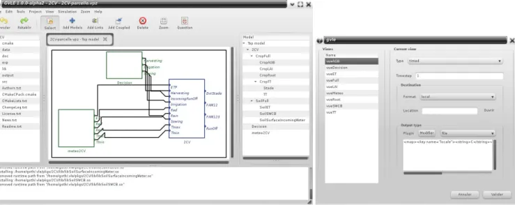
Figure 5. These pictures show the GVLE modeling tool. In the left picture, GVLE is used to build hierarchy of models and connections, to attach behaviours, experimental conditions and observations to atomic models. In the right picture is used to parametrize the observer models.
Finally, from the user point of view of the M&S framework the delivery of a reliable service of observation that can be used either in simple case or in complex experimental frame is a true advantage when the need is to study simulations of heterogeneous coupled models.
REFERENCES
[1] B. Bont´e, R. Duboz, G. Quesnel, and J.P. M¨uller. Recursive simulation and experimental frame for multiscale simulation. In Summer Computer Simulation Conference, pages 164–172, Istanbul, Turkey, July 2009.
[2] P. Chabrier, F. Garcia, R. Martin-Clouaire, G. Quesnel, and H. Raynal. Toward a simulation modeling platform for study-ing croppstudy-ing systems management: the record project. In Inter-national Congress on Modelling and Simulation, InterInter-national Society for Computer Simulation, pages 10 –13, Christchurch. New Zealand., 2007.
[3] A.C.H. Chow and B.P. Zeigler. Parallel DEVS: a parallel, hi-erarchical, modular, modeling formalism. In Proceedings of the 26th conference on Winter simulation, pages 716–722, Or-lando, Florida, United States, 1994.
[4] David Goldberg. What every computer scientist should know about floating-point arithmetic. ACM Computing Surveys, 23:5–48, March 1991.
[5] A. Gosavi. Simulation-Based Optimisation – Parametric Op-timization Techniques and Reinforcement Learning. Kluwer Academic Publishers, 2003.
[6] J. Himmelspach and A. M. Uhrmacher. The JAMES II Frame-work for Modeling and Simulation. In International Workshop on High Performance Computational Systems Biology, pages 101–102, 2009.
[7] Edward A. Lee. Overview of the Ptolemy Project, july 2003. Technical Memorandum No. UCB/ERL M03/25.
[8] G. Quesnel, R. Duboz, and ´E. Ramat. The Virtual Laboratory Environment – An operational framework for multi-modelling, simulation and analysis of complex dynamical systems. Sim-ulation Modelling Practice and Theory, 17:641–653, April 2009.
[9] R Development Core Team. R: A Language and Environment for Statistical Computing. R Foundation for Statistical Com-puting, Vienna, Austria, 2006. ISBN 3-900051-07-0. [10] J. Ribault, O Dalle, D. Conan, and S. Leriche. OSIF: a
framework to instrument, validate, and analyze simulations. In SIMUTools ’10 Proceedings of the 3rd International ICST Conference on Simulation Tools and Techniques, 2010. [11] Michael M. Tiller. Introduction to Physical Modeling with
Modelica. Kluwer Academic, 2001.
[12] M. K. Traor´e and B. P. Zeigler. Experimental Frames Method-ology. In NSF Workshop on Modeling and Simulation for Design of Large Software-Intensive Systems: Challenges and New Research Directions. DLS03, Tucson, AZ, USA, Decem-ber 2003.
[13] B. P. Zeigler, D. Kim, and H. Praehofer. Theory of model-ing and simulation: Integratmodel-ing Discrete Event and Continuous Complex Dynamic Systems. Academic Press, 2000.