Correlation maps: A compressed access method
for exploiting soft functional dependencies
The MIT Faculty has made this article openly available.
Please share
how this access benefits you. Your story matters.
Citation
Hideaki Kimura, George Huo, Alexander Rasin, Samuel Madden, and
Stanley B. Zdonik. 2009. Correlation maps: a compressed access
method for exploiting soft functional dependencies. Proc. VLDB
Endow. 2, 1 (August 2009), 1222-1233.
As Published
http://dx.doi.org/10.14778/1687627.1687765
Publisher
Association for Computing Machinery (ACM)
Version
Author's final manuscript
Citable link
http://hdl.handle.net/1721.1/90382
Terms of Use
Creative Commons Attribution-Noncommercial-Share Alike
Correlation Maps: A Compressed Access Method for
Exploiting Soft Functional Dependencies
Hideaki Kimura
George Huo
Alexander Rasin Samuel Madden Stanley B. Zdonik
Brown University Google, Inc. Brown University MIT CSAIL Brown University
[email protected] [email protected] [email protected] [email protected] [email protected]
ABSTRACT
In relational query processing, there are generally two choices for access paths when performing a predicate lookup for which no clustered index is available. One option is to use an unclustered index. Another is to perform a complete sequential scan of the table. Many analytical workloads do not benefit from the availability of unclustered indexes; the cost of random disk I/O becomes prohibitive for all but the most selective queries.
It has been observed that a secondary index on an unclustered attribute can perform well under certain conditions if the unclus-tered attribute is correlated with a clusunclus-tered index attribute [4]. The clustered index will co-locate values and the correlation will localize access through the unclustered attribute to a subset of the pages. In this paper, we show that in a real application (SDSS) and widely used benchmark (TPC-H), there exist many cases of attribute correlation that can be exploited to accelerate queries. We also discuss a tool that can automatically suggest useful pairs of correlated attributes. It does so using an analytical cost model that we developed, which is novel in its awareness of the effects of clustering and correlation.
Furthermore, we propose a data structure called a Correlation Map (CM) that expresses the mapping between the correlated attributes, acting much like a secondary index. The paper also discusses how bucketing on the domains of both attributes in the correlated attribute pair can dramatically reduce the size of the CM to be potentially orders of magnitude smaller than that of a secondary B+Tree index. This reduction in size allows us to create a large number of CMs that improve performance for a wide range of queries. The small size also reduces maintenance costs as we demonstrate experimentally.
1.
INTRODUCTION
Correlations appear in a wide range of domains, including product catalogs, geographic databases, census data, and so on [4, 9]. For example, demographics (race, income, age, etc.) are highly correlated with geography; price is highly correlated with product industry; in the natural world, temperature, light, humidity, energy, and other parameters are often highly correlated; in the stock market, trends in one security are often closely related to those of others in similar markets.
Recent years have seen the widespread recognition that corre-lations can be effectively exploited to improve query processing performance [4, 9, 21, 17, 7]. In particular, if a column C1 is
Permission to copy without fee all or part of this material is granted provided that the copies are not made or distributed for direct commercial advantage, the VLDB copyright notice and the title of the publication and its date appear, and notice is given that copying is by permission of the Very Large Data Base Endowment. To copy otherwise, or to republish, to post on servers or to redistribute to lists, requires a fee and/or special permission from the publisher, ACM.
VLDB ‘09,August 24-28, 2009, Lyon, France
Copyright 2009 VLDB Endowment, ACM 000-0-00000-000-0/00/00.
correlated with another column C2 in table T , then it may be
possible to use access methods (such as clustered indexes) on C2
to evaluate predicates on C1, rather than using the access methods
available for C1alone [4, 21, 17, 7].
In this paper, we focus on a broad class of correlations known as soft functional dependencies (soft FDs), where the values of an attribute are well-predicted by the values of another attribute. For example, if we know that the value of city is Boston, we know with high probability but not with certainty that the value of stateis Massachusetts (since there is a large city named Boston in Massachusetts and a much smaller one in New Hampshire). Such soft FDs are a generalization of hard FDs, where one attribute is a perfect predictor of another attribute.
Previous work has observed that soft FDs can be exploited by in-troducing additional predicates into queries [4, 7] when a predicate over only one correlated attribute exists. For example, if a user runs the query SELECT * FROM emp WHERE city=’boston’, we can rewrite the query as
SELECT * FROM emp WHERE city=’boston’
AND (state=’MA’ or state=’NH’)
This will allow the query optimizer to exploit access methods, such as a clustered index on state, that it would not otherwise choose for query processing. Estimating and improving the performance of such secondary index lookups in the presence of correlations is our primary goal in this work.
In this work, we make three principal contributions beyond existing approaches: first, we describe a set of algorithms to search for soft functional dependencies that can be exploited at query execution time (e.g., by introducing appropriate predicates or choosing a different index). Without such a mechanism it is difficult for the query planner to identify predicates to introduce to exploit a broad array of soft FDs. Our algorithms are more general than pre-vious approaches like BHUNT [4] because we are able to exploit correlations in both numeric and non-numeric (e.g. categorical) domains. Our algorithms are also able to identify multi-attribute functional dependencies, where two or more attributes A1. . . Anare
stronger determinants of the value of an attribute B than any of the attributes in A1. . . Analone. Consider a database of cities, states,
and zipcodes. The pair (city, state) is clearly a better predictor of zipcode than city or state alone, as there are many cities in the US named “Fairview” or “Springfield” but there is typically only one city with a given name in a particular state.
Our second major contribution is to develop an analytical cost model to predict the impact of data correlations on the performance of secondary index look-ups. Although previous work has exam-ined how correlations affect query selectivity, our cost model is the first to describe actual query execution using statistics that are practical to calculate on large data sets. Furthermore, the model is general enough that we use it in our algorithms to search for soft FDs as well as during query optimization. We show that this model is a good match for real world performance.
Our third contribution is to observe that to effectively exploit the correlations identified by any search algorithm (including ours or those in previous work), it may be necessary to create a large number of secondary indexes (one per pair of correlated attributes). Such indexes can be quite large, consuming valuable buffer pool space and dramatically slowing the performance of updates, possi-bly obviating the advantages gained from correlations. We address this concern by proposing a compressed index structure called a correlation map, or CM, that compactly represents correlations. By avoiding the need to store an index entry for every tuple and by employing bucketing techniques, we are able to keep the size of CMs to less than a megabyte even for multi-gigabyte tables, thus allowing them to easily fit into RAM.
CMs are simply a mapping from each distinct value (not tuple) uin the domain of an attribute Auto pages in another attribute Ac
that contain tuples co-occurring with u in the database. Given a clustered attribute Ac(for which their exists a clustered index), we
call attribute Au the unclustered attribute. Queries over Au can
be answered by looking up the co-occurring values of u in the clustered index on Acto find matching tuples.
We also evaluate the effectiveness of exploiting correlated at-tributes on several data sets, coming from TPC-H, eBay, and the Sloan Digital Sky Survey (SDSS). We show that correlations signif-icantly improve query processing performance on these workloads. For example, we show that in a test benchmark with 39 queries over the SDSS data set, we are able to obtain more than a 2x performance improvement on 13 of the queries and greater than 16x improvement on 5 of the queries by building an appropriately correlated clustered index on one of the tables. We then show that CMs can capture these same gains during query processing with orders of magnitude less storage overhead. We show that maintenance of CMs (including overheads for recovery) slows the performance of update queries dramatically less than traditional B+Trees. For example, we find that in the Experiment 3 of Section 7.2 with 10 CMs or unclustered B+Trees, CMs can sustain an update rate of 900 tuples per second, whereas B+Trees are limited to 29 per second, a factor of 30 improvement.
2.
RELATED WORK
There is a substantial body of prior work on exploiting correla-tions in query processing. One can view our work as an extension of approaches from the field of semantic query optimization (SQO); there has been a long history of work in this area [21, 8, 12, 19]. The basic idea is to exploit various types of integrity constraints— either specified by the user or derived from the database—to eliminate redundant query expressions or to find more selective access paths during query optimization.
Previous SQO systems have studied several problems that bear some resemblance to correlation maps. Cheng et al. [17] describe predicate introductionas one of their optimizations (which was originally proposed by Chakravarthy et al [21] and is the same technique we use in rewriting queries), in which the SQO injects new predicates in the WHERE clause of a query based on constraints that it can infer about relevant table attributes; in this case they use logical or algebraic constraints (as in Gryz et al. [7]) to identify candidate predicates to insert.
BHUNT [4] also explores the discovery of soft constraints, focusing on algebraic constraints between pairs of attributes. The authors explain how to use such constraints to discover access paths during query optimization. For example, the distribution of (delivery date – ship date) in a sales database may cluster around a few common values – roughly 4 days for standard UPS, 2 days for air shipping, etc, that represent “bumps” in delivery dates relative to ship dates. The idea is a generalization of work by Gryz
et al. [7], who propose a technique for deriving “check constraints,” which are basically linear correlations between attributes with error bounds (e.g., salary= age∗1k±20k). Godfrey et al. [15] have also looked at discovering and utilizing “statistical soft constraints” are similar to bumps with confidence measures in BHUNT.
If the widths of the bumps are chosen wisely, BHUNT can capture many algebraic relationships between numeric columns. The authors describe how such constraints can be included in the WHEREclause in a query to allow the optimizer to use alternative ac-cess paths (for example, by adding predicates like deliveryDate BETWEEN shipDate+1 and shipDate+3). Like BHUNT, CMs also are used to identify constraints that can be used to optimize query execution. Unlike BHUNT, CMs are more general because they are not limited to algebraic relations over ordered domains (e.g., BHUNT cannot find correlations between states and zip codes). BHUNT also does not address multi-dimensional corre-lations or bucketing, which are a key focus of this paper.
The CORDS system in IBM DB2 [9] builds on the work of BHUNT by introducing a more sophisticated measure of attribute-pair correlation that captures non-numeric domains. CORDS calculates statistics over samples of data from pairs of attributes that satisfy heuristic pruning rules, and it determines soft (nearly unique) keys, soft FDs, and other degrees of correlation. CMs and CORDS are similar in their measure of soft FD strength and their use of a query training set to limit the search space over candidate attribute sets. Relative to CORDS, our work adds our compressed correlation map structure (CMs), a complete cost model and set of methods to exploit the discovered correlations in query processing using CMs or secondary indices, and a set of techniques to recommend secondary indices / CMs to build. CORDS, on the other hand, focuses on using correlation statistics to improve selectivity estimation during query optimization, and it does not examine how to maintain the information necessary for use during query execution. CORDS also does not find multi-dimensional correlations or explore bucketing. Oracle 11g and PostgreSQL have related statistics [3, 2], but they are used only for choosing execution plans, too.
Chen et al. describe an approach called ADC Clustering that is related in that it addresses the poor performance of secondary indexes in data warehousing applications [22]. ADC Clustering aims to improve the performance of queries in a star schema by physically concatenating the values of commonly queried dimen-sion columns that have restrictions into a new fact table, and then sorting on that concatenation. Though correlations in the underlying data play a major role in the performance of their approach, ADC Clustering does not directly measure correlations or model how they affect query performance.
When paired with an appropriate clustered index, a CM on an unclustered attribute may replace a much larger secondary index structure (such as a B+Tree or bitmap index) by serving as a lossy representation of the index. There has been work on approximate bitmap index structures (e.g. [20]), where Bloom filters are used to determine which tuple IDs may contain a particular attribute value. These techniques do not achieve as much compression as CMs because they represent maps of tuples instead of values. Also, false positives in approximate bitmaps will result in a randomly scattered set of records that may match a given lookup, whereas bucketing in CMs results in a contiguous range of clustered attribute records that may match a lookup. Work on approximate bitmaps also does not discuss how to choose the index size (the bin width, in our work) to preserve correlations, as we do. Existing work on non-lossy index compression, such as prefix compression [18] cannot achieve anywhere near the same compression gains; our experiments with
gzip and index compression on our data sets suggest they yield typical size reductions factors of 3–4.
Microsoft SQL Server has a similar technique called datetime correlation optimization[1]. It maintains a small materialized view to store co-occurring values of two datetime columns. When one of the datetime columns is the clustered index key and the other is predicated in a query, the MV is internally used to infer an additional predicate on the clustered index. Though the approach is related to ours, it is unable to capture general correlations. For example, SQL Server is unable to exploit the state-city correlation described in Figure 4 because it supports only datetime columns. In data-warehouse queries, it is unusual for both the clustered key and predicated key to have datetime types. Second, it cannot capture multi-attribute correlations. For example, the (longitude, latitude)→zipcode example described in Section 6 is inexpressible by SQL Server. Detecting and exploiting such correlations in a scalable way requires a sophisticated analysis. Third, it lacks an adaptive bucketing scheme as described in Section 6 to utilize correlations over a wide range of attribute domains. SQL Server always buckets datetime values into month-long ranges. Without an adaptive bucketing scheme, a system would not be able to op-timize both the index size (and thus maintenance costs) and query performance unless the attribute domains are evenly and sparsely distributed. Last, SQL Server does not publish an analytic cost model to evaluate the benefit of correlations, which is required to determine the pairs of attributes to exploit. To realize these features, we establish a correlation-aware cost model to evaluate the benefit of correlations and the CM advisor to detect general correlations and design proper bucketing schemes based on workload queries.
3.
B+TREES AND CORRELATIONS
We begin with a brief discussion of the costs of conventional database access methods and how they are affected by correlations, before presenting a cost model for predicting the effect of such access methods (Section 4) and a discussion of our compressed CM structure (Section 5).
For selections when a clustered index is unavailable, a database system has two choices: it may choose to perform a full table scan or use a secondary B+Tree index, if one exists. The cost of each access method depends on well understood factors—table sizes, predicate selectivities, and attribute cardinalities—as well as less well understood factors like correlations. To understand these factors, we begin with a simple cost model and show how it changes in the presence of correlations.
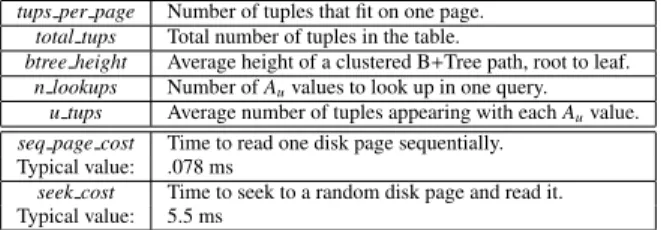
In the following discussion, we assume a table with clustered attribute Acand secondary attribute Auon which we query. Table 1
summarizes the statistics that we calculate over each table. For the hardware parameters seek cost and seq page cost the table shows measured values from our experimental platform. We assume that all of the access methods are disk-bound.
Consider a sequential table scan. A table scan incurs no random seek costs, but it must read each page in the table in order of the clustered key. The number of pages p in a table istups per pagetotal tups . The costscanof scanning a table is then just seq page cost × p. We note
here that this model is oblivious to external factors such as disk fragmentation and as such underestimates the true cost of a scan in a real database implementation; our numbers show true scan cost to be approximately 10% higher in our implementation.
As our goal in this paper is to explore secondary index costs, we present cost models for secondary index accesses in the next two sections, and then show how correlations affect such accesses.
3.1
Pipelined Index Scan
A secondary B+Tree index is the standard alternative to a table
Table 1: Statistics and parameters used in analytical model. tups per page Number of tuples that fit on one page.
total tups Total number of tuples in the table.
btree height Average height of a clustered B+Tree path, root to leaf. n lookups Number of Auvalues to look up in one query.
u tups Average number of tuples appearing with each Auvalue.
seq page cost Time to read one disk page sequentially. Typical value: .078 ms
seek cost Time to seek to a random disk page and read it. Typical value: 5.5 ms
scan, providing an efficient way to access a disk page containing a particular unclustered attribute value. While the B+Tree identifies the locations where relevant tuples can be found, it cannot guar-antee that the tuples are accessed without interleaving seeks. This is because the table may be clustered on a different attribute, and a scan may result in tuple accesses scattered randomly across the physical pages on disk.
In general, if the query executor uses a pipelined iterator model (e.g., performing repeated probes into an index that is the inner relation of a nested loops join) to feed tuples to operators, then a B+Tree operator may need to access unclustered attribute values in an order over which it has no control. If we ignore correlations between the unclustered and clustered attributes, then, each new input value will send the operator on btree height random seeks. The approximate cost of n lookups is then:
costuncorrelated= (n lookups)(u tups)(seek cost)(btree height)
Since a random seek is so expensive, a pipelined secondary B+Tree operation only makes sense for a small number of specific value lookups. When the set of values to look up is available up front (as in a blocked index nested loops join, or a range selection over a base table), the standard optimization is to sort the index keys before looking them up in the hash table. We call this a sorted index scan.
3.2
Sorted Index Scan
When the set of all Au values satisfying the predicate is known
up front, the query executor can perform a number of lookups on the unclustered B+Tree and assemble a list of record IDs (RIDs) of all of the actual data tuples in the heap files. The RIDs can then be sorted and de-duplicated. This allows the B+Tree to perform a single sequential sweep to access the heap file, rather than a separate disk seek for each unclustered index lookup. This sweep always performs at least as fast as a sequential scan; it will be faster if it can seek over large regions of the file.
The sorting itself can be implemented in a variety of ways. For example, PostgreSQL uses the index to build a bitmap (with one bit per tuple) indicating the pages that contain records that match predicates [16]. It then scans the heap file sequentially and reads only the pages where corresponding bits are set in the bitmap. In practice, the CPU costs for sorting the offsets is typically negligible compared to the I/O costs saved by the improved access pattern.
3.3
The Effect of Correlations
In this section, we show that the performance of a sorted index scan is highly dependent on correlations between the clustered and unclustered values. In particular, a sorted index scan behaves especially nicely when the clustered table value is a good predictor for an unclustered value. To illustrate this, in Figure 1 we visualize the distribution of page accesses when performing lookups on an unclustered B+Tree over the lineitem table from the TPC-H benchmark. The figure shows the layout of the lineitem table as a horizontal array of pages numbered 1 . . . n. Each black mark indicates a tuple in the table that is read during lookups of three distinct values of the unclustered attribute (either suppkey or shipdate). The four rows represent four cases (in vertical order):
2. a lookup on suppkey; table is not clustered
3. a lookup on shipdate; table is clustered on receiptdate 4. a lookup on shipdate; table is not clustered
The suppkey is moderately correlated with partkey, as each sup-plier only supplies certain parts. The shipdate and receiptdate are highly correlated as most products are shipped 2, 4, or 5 days before they are received.
In both cases, where correlations are present, the sorted index scan visits a small number of sequential groups of pages com-pared to numerous scattered pages when no correlation exists. Particularly striking is the high-correlation case (shipdate and receiptdate), where the sorted index scan only performs a handful of large seeks to reach long sequential groups of pages. The overall cost of accessing the index on shipdate when the table is clustered on receiptdate is about 1/20 the cost of accessing it when no clustering is used on the table.
Page 0 . . . n
partkey (Ac) vs
suppkey (Au)
receiptdate (Ac)
vs shipdate (Au)
Figure 1: Access patterns in lineitem table for an unclustered B+Tree lookup on Au (suppkey/shipdate) with and without
clustering on correlated attribute Ac(partkey/receiptdate).
3.4
Experiments
Based on the intuition about the potential benefit of correlations described above, in this section we describe two experiments that demonstrate the actual benefit correlations yield when running queries with unclustered B+Trees We describe our experimental setup and these data sets in more detail in Section 7.
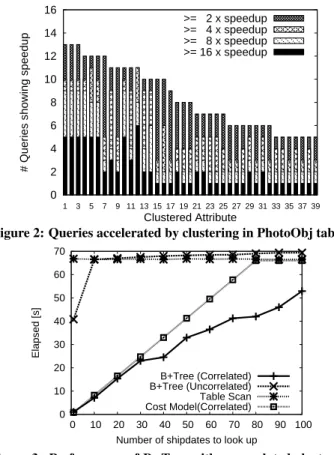
Varying the clustered attribute: Figure 2 shows the result of an experiment conducted on the SDSS data set to demonstrate that clustering on one well-chosen attribute can speed up many queries. For this experiment, we devised a simple benchmark consisting of 39 queries, each of which has a predicate over one of the attributes in the PhotoObj table of the SDSS data set with 1% selec-tivity. This table contains information about the optical properties of various celestial objects, including their color, brightness, and so on. Queries selecting objects with different combinations of these attributes are very common in SDSS benchmarks [11].
We then clustered the table in 39 different ways (once on each of the 39 attributes used in our test queries), and ran all 39 queries over each clustering to measure the benefit that correlations can offer.
Figure 2 shows the number of queries that run at least a factor of 2, 4, 8, or 16 times faster than a pure table scan (or an unclustered sorted index scan) when using a secondary index lookup for each choice of clustered attribute. The clustered attribute varies on the horizontal axis. For example, attribute 1 (fieldID) is highly correlated with 12 attributes and clustering on it sped up querying on 13 queries by at least a factor of two over a table scan, with 5 of them exhibiting more than a factor of 16 speed-up.
Introducing correlated clustering: In this experiment we look at the TPC-H attributes shown in Figure 1. We again highlight the benefits of a good clustered index choice.
We measured the performance of queries over TPC-H data with two different clustering schemes on the PostgreSQL database. In the first, the lineitem table is clustered on receiptdate, which is correlated with shipdate. In the second, we cluster on the primary key – (orderkey, linenumber) – which is not correlated with shipdate. In both cases, we create a standard secondary B+Tree on shipdate. The query used in the experiment is:
0 2 4 6 8 10 12 14 16 1 3 5 7 9 11 13 15 17 19 21 23 25 27 29 31 33 35 37 39
# Queries showing speedup
Clustered Attribute >= 2 x speedup >= 4 x speedup >= 8 x speedup >= 16 x speedup
Figure 2: Queries accelerated by clustering in PhotoObj table
0 10 20 30 40 50 60 70 0 10 20 30 40 50 60 70 80 90 100 Elapsed [s]
Number of shipdates to look up B+Tree (Correlated) B+Tree (Uncorrelated) Table Scan Cost Model(Correlated)
Figure 3: Performance of B+Tree with a correlated clustered index on shipdate vs. an uncorrelated clustered index
SELECT AVG(extendedprice * discount) FROM LINEITEM WHERE shipdate IN [list of 1 to 100 random shipdates]
As the graph in Figure 3 shows, the correct choice for the clustered attribute can significantly improve the performance of the secondary B+Tree index. For the uncorrelated case the per-formance degrades rapidly, reaching the cost of a sequential scan for queries with more than 4 shipdates. This happens because the query on the uncorrelated attribute selects receiptdate values that are scattered (approximately 7000 per shipdate), so the bitmap scan access pattern touches a large fraction of the lineitem table. We have observed the same behavior in other commercial database products. Figure 3 also shows that we have a cost model that is able to accurately predict the performance of unclustered B+Trees in the presence of correlations – we present this model in detail in the next section.
These experiments show that, if we had a way to discover these correlations, substantial performance benefits are possible.Hence, in the next few sections, we focus on our methods for discovering such correlations. In particular, we show how to extend our ana-lytical cost model to capture the effect of correlations (Section 4), our algorithms for building compact CM indices (Section 5), and finally our approach for discovering correlations (Section 6).
4.
MODEL OF CORRELATION
In this section, we present our model for predicting the cost of sorted index lookups in the presence of correlations. To the best of our knowledge, this is the first model for predicting query costs that embraces data correlations. As a result, it is substantially more accurate than existing cost models in the presence of strongly correlated attributes.
Table 2: Statistics used to measure attribute correlation. c tups Average number of tuples with each Acvalue.
As shown in Table 2, we introduce two additional statistics that capture a simple measure of correlation between Au and Ac. The
c per uvalue indicates the average number of distinct Acvalues
that appear in some tuple with each Au value. The same measure
was proposed in CORDS [9] as the strength of a soft FD, where it was used for finding strongly correlated pairs of attributes to update join selectivity statistics rather than building a cost model.
4.1
Index Lookups with Correlations
Suppose that we are using a secondary B+Tree that sorts its disk accesses when looking up a set of Au values as described in
Section 3.2. For each Au value v, the query must visit c per u
different clustered attribute values. We need to perform one clustered index lookup to reach each of these clustered attribute values. Once we reach a clustered value, we need to scan at most c pagespages to guarantee finding each tuple containing v. As before, we take the cost of an index lookup to be btree height disk seeks. For each Acvalue, we have to scan c tups/tups per page
pages. Finally, as with an uncorrelated sorted index scan, when we scan a large fraction of the file, the access pattern becomes gradually closer to a full table scan. Hence, the index scan is upper bounded by costscan. These observations lead to the following
expression for the cost of n lookups on a secondary B+Tree with correlations:
c pages= c tups/tups per page
costsorted= min((n lookups)(c per u)[(seek cost)(btree height)
+ (seq page cost)(c pages)], costscan)
One simplification in our model is that we ignore the potential overlap between the sets of Ackeys associated with two particular
Au values. In other words, if one Au value maps to n different
Ac values on average, then it is not true in general that two Au
values map to 2n different Acvalues. Our model may overestimate
the number of Acvalues involved, and thus the cost of secondary
indexes. This is a concern, for example, when evaluating a range predicate over an unclustered attribute that has linear correlation with the clustered attribute (e.g., order receipt dates will overlap heavily for a range of ship dates).
This cost model captures two key facts: first, when both c per u and c pages are small, the cost of an individual secondary index lookup is not much more than the cost of a lookup on a clustered index (which costs btree height seeks plus a scan of c pages). c per uwill be small when there are few values in the clustered attribute, or when there is a correlation between the clustered attribute and the unclustered attribute. Second, if c per u is small because the clustered attribute is few-valued, then c pages will likely be large, driving up the cost of each unclustered index access as it will scan a large range of the table.
On the other hand, if c per u is small due to correlations, c pages is not necessarily large. Hence, if we cluster a table on an attribute that has:
1. A small c pages value and,
2. Correlations to many unclustered attributes (i.e., with a small c per uvalue for many unclustered attributes),
then we can expect to be able to exploit this clustering to get good performance from many different secondary indices.
4.2
Implementing The Cost Model
To obtain performance predictions from this cost model, we have developed a tool that scans existing tables and calculates the statistics needed by the cost model. Our approach for doing this is quite simple and uses a sampling-based method to reduce the heavy cost of exact parameter calculation.
Given these statistics and measurements of underlying hardware properties, the cost model can predict how much (or if) a given pair of attributes benefits from an unclustered index. The database administrator can use these measurements to choose to build unclustered indexes and to cluster tables on high-benefit attribute pairs that the application is likely to query. In Section 7, we present the plots predicted by our cost model alongside our empirical results.
The key measure of correlation that our model relies on is the c per ustatistic. As c per u is the average number of distinct Ac
values for each Auvalue, we can calculate its value based on the
cardinalities of columns, as follows (this approach is similar to that presented in [9]). We write the number of distinct values over a pair of attributes Aiand Ajas D(Ai, Aj) and the number of distinct
values over a single attribute as D(Ai). Then we can write:
c per u=D(Au, Ac) D(Au)
The basic problem of estimating the cardinality of a column has had extensive treatment in both the database and statistics communities, where it is known as the problem of estimating the number of species (e.g. [10]).
For estimating single-attribute cardinality, we use the Distinct Sampling (DS) algorithm by Gibbons [6], which computes esti-mates that are far more accurate than pure sampling-based ap-proaches at a cost of one full table scan. We choose DS over less costly sampling schemes because an error in cardinality estimation for single attributes may cause substantial errors in later database design phases (alternatively, the system catalogs may maintain this statistic accurately).
In Section 6 we present our CM advisor that recommends multi-column composite indexes. It is not feasible to use DS for estimating the cardinality of all attribute combinations that our advisor considers, so to estimate composite c per u measurements we use the Adaptive Estimator (AE) algorithm [13]. AE estimates composite attribute cardinalities based on a random data sample; we sacrifice some accuracy, but it is very fast because the sample can be kept in memory. These samples are randomly collected during the DS table scan, yielding an optimum random sample as described in [14].
5.
COMPRESSING B-TREES AS CMS
We have shown the potential to exploit correlations to make unclustered B+Trees perform more like clustered B+Trees, and we now turn our attention to describe how to efficiently store many unclustered B+Trees in a database system. Our approach uses a compressed B+Tree-like structure called a Correlation Map (CM) that works especially well in the presence of correlations. Compressing secondary indexes is not a new concept: several approaches have been explored in prior work [18]. The goals of compression are twofold; first, compression saves disk space, which can be prohibitive when considering numerous indexes on large datasets. Second, compression improves system performance by reducing I/O costs associated with using indexes and by reduc-ing pressure on the buffer pool.
Although disk space is becoming cheaper every day, it is still a limited resource. For large data warehouses in real applications, having many B+Tree indexes can easily require petabytes of disk space and thus does not scale [11]. Existing lossless index compression might achieve up to a 4x reduction in space while, as we show in our experimental section, CMs can reduce index sizes by 3 orders of magnitude. There is an obvious advantage to reducing secondary index sizes – the database requires less disk
space and index lookups during query processing consume fewer I/O operations. However, an even more significant improvement comes from reduced index maintenance costs.
Indexes have to be kept up-to-date as the underlying data change through inserts or deletes. Accessing the disk on every update is prohibitively expensive. Thus, the universally applied solution is to keep modified pages in memory and delay writing to disk for as long as possible. Unfortunately, RAM is a much more limited resource than disk space and only a small fraction of a typical B+Tree can be cached. As we show in Experiment 3 of Section 7.2, maintaining as few as 5 or 10 B+Trees can lead to a dramatic slowdown in overall system performance. CMs on the other hand can be usually be fully cached in memory as they are quite small; this leads to substantially lower update cost. This means that it is realistic to maintain a large number of CMs, whereas it may not be practical to maintain many conventional B+Trees. In the rest of this section, we describe how CMs are structured, built, and used.
5.1
Building and Maintaining CMs
Given that the user wants to build a CM over an attribute T.Auof
a table T (we call this is the CM Attribute), with a clustered attribute T.Ac, the CM is simply a mapping of the form u → Sc, where
1. u is a value in the domain of T.Au, and
2. Scis a set of values in the domain of T.Acs.t.there exists a
tuple t ∈ T of the form (t.Au= u, t.Ac= c, . . .) ∀c ∈ Sc.
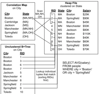
For example, if there is a clustered index on product.state, a CM on product.city might contain the entry “Boston → {NH,MA},” indicating that there is a city called Boston in both Massachusetts and New Hampshire.
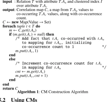
The algorithm for building a CM is shown in Algorithm 1. The algorithm works as follows: once the administrator issues a DDL command to create a CM, the system scans the table to build the mapping (line 1). As the system scans the table, it looks up the CM key value in the mapping and adds the clustered index key to the set of key values (line 1). The system tracks the number of times a particular pair of (uncorrelated, correlated) values occurs using a “co-occurrence” count, which is initialized to 1 (line 1) and incremented as needed (line 1).
The number of times a particular correlated value occurs with each uncorrelated value in the table is needed for deletions. When a tuple t is deleted, the CM looks up the mapping mAu for the uncorrelated attribute value and decrements the count c for the correlated value t.Ac. When c reaches 0, the value t.Acis removed
from mAu.
The insertion algorithm is very similar to the algorithm for building the table. The main loop (line 1 in Algorithm 1) is simply repeated for each new tuple that is added. Updates can be treated as a delete and an insert.
Since a CM is just a key-value mapping from each unclustered attribute value to the corresponding clustered attribute values, it can be physically stored using any map data structure. This is convenient because database systems provide B+Trees and Hash Indexes that can be used for this purpose. In our implementation, we physically represent a CM using a PostgreSQL table. Whenever a tuple is inserted, deleted, or modified, the CM must be updated as discussed above. Because the CM is relatively compact (containing one key for each value in the domain of the CM attribute, which in our experiments occupy 0.1–1 MB for databases of up to 5 GB), we expect they can generally be cached in memory. Rather than modify PostgreSQL internals, we implemented our own front-end client that caches CMs (see Section 7.1). We report the sizes of CMs for several datasets in our experimental evaluation in Section 7, showing that they are often much more compact than the equivalent B+Tree.
input : Relation T with attribute T.Auand clustered index I
over attribute T.Ac
output: Correlation map C, a map from T.Auvalues to
co-occurring T.Acvalues, along with co-occurrence
count.
C ←new Map(Value → Set) foreach tuple t ∈ T do
m ← C.get(t.Au)
if (m.get(t.Ac)= null) then
/* Add fact that t.Ac co-occurred with t.Au
to mapping for t.Au, initializing
co-occurrence count to 1 */
m.put(t.Ac, 1)
end else
/* Increment co-occurrence count for t.Ac
in mapping for t.Au */
cnt ← m.get(t.Ac)
m.put(t.Ac, cnt + 1)
end end return C
Algorithm 1: CM Construction Algorithm
5.2
Using CMs
The API for performing lookups on the CM is straightforward; the CM implements a single procedure, cm lookup({vu1. . . vuN}).
It takes a set of N CM attribute values as input and returns a list of clustered attribute values that co-occur with {vu1. . . vuN}. These
clustered attribute values are determined by taking the union of the clustered attribute values returned by a CM lookup on each unclustered value vui.
Given a list of clustered attribute values to access, the system then performs a sorted index scan on the clustered index. Return values from this scan must be filtered by predicates over the CM attribute, since some values in the clustered index may not satisfy the unclustered predicates – for example, a scan of the states “MA” and “NH” to find records with city “Boston” will encounter many records from non-satisfying cities (e.g., “Manchester”.)
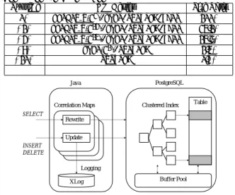
Figure 4 illustrates an example CM and how it guides the query executor. A secondary B+tree index on city is a dense structure, containing an entry for every tuple appearing with each city. In order to satisfy the “Boston” or “Springfield” predicate using a standard B+Tree, the query engine uses the index to look up all corresponding rowids. The equivalent CM in this example contains all unique pairs (city, state). To satisfy the same predicate using a CM, the query engine looks up all possible state values corresponding to “Boston” or “Springfield”. The resulting values (“MA”, “NH”, “OH”) correspond to 3 sequential ranges of rowids in the table. These are then scanned and filtered on the original city predicate. Notice that the CM scans a superset of the records accessed by the B+Tree, but that it contains fewer entries.
5.3
Discussion
CMs capture the correlation between the indexed attribute and the clustered attribute. If the two attributes are well-correlated, each value of the CM attribute will co-occur with only a few values in the clustered attribute, whereas if they are poorly correlated, the CM attribute will co-occur with many clustered attribute values. The degree of compression obtained by replacing a B+Tree with a CM is determined by the degree of correlation as the CM needs to store every unique pair of attributes (Au, Ac).
We’ve already seen that CM performance is well-predicted by c per u. However, there is another condition that affects the performance of correlation maps: they only perform well when the set of relevant clustered attribute values covers a relatively small fraction of the entire table. To see this, consider a correlation with
Heap File clustered on State Unclustered B+Tree on City Toledo 10 9 Springfield Manchester 6 4 3 RID Boston Jackson Manchester 2 1 Springfield Boston 7 City 5 8 Boston Boston Correlation Map on City City State SELECT AVG(salary) FROM people WHERE city = 'Boston' OR city = 'Springfield' 10 OH Toledo $70K $95K 9 OH Springfield $60K 8 NH Manchester MA $40K 7 State Boston MA $110K City Manchester 2 4 Boston $25K 1 $80K NH 6 Jackson Springfield $90K MS MA RID NH Boston $50K $45K Boston 3 Salary 5 MN {MS} Jackson {OH} Toledo {MA,OH} Springfield {MN,NH} Manchester {MA} Cambridge {MA,NH} Boston Scan MA,NH, OH Lookup individual tuples that match
(sorting RIDs) first)
Figure 4: Diagram illustrating an example CM and its use in a query plan, and comparing to the use of a conventional B+Tree a table clustered on a small-domain attribute, such as gender. Even if the gender attribute is highly correlated with some unclustered attribute, the correlation is unlikely to reduce access costs for most scans of the unclustered attribute, since the system would have to scan about 50% of the table using the CM.
We now briefly describe how CMs can be further compressed through bucketing. An extensive treatment of our approach to bucketing over one or multiple attributes can be found in Section 6.
5.4
Bucketing CMs
The basic CM approach described in the previous section works well for attributes where the number of distinct values in the CM attribute or the clustered attribute are relatively small. However, for large attribute domains (such as real-valued attributes), the size of the CM can grow quite unwieldy (in the worst case having one entry for each tuple in the table). Keeping a CM small is important to keep the performance benefits outlined above.
We can reduce the size of a CM by “bucketing” ranges of the unclustered attribute together into a single value. We can compress ranges of the clustered attribute stored in the CM similarly. For example, suppose we build a CM on the attribute temperature with a clustered index on humidity (these attributes are often correlated, with lower temperatures bringing lower humidities). For example, given the unbucketed CM on the left, we can bucket it into the 1oCor 1% intervals shown on the right via truncation:
{12.3oC} → {17.5%, 18.3%} {12.7oC} → {18.9%, 20.1%} {14.4oC} → {20.7%, 22.0%} {14.9oC} → {21.3%, 22.2%} {17.8oC} → {25.6%, 25.9%} {12 − 13oC} → {17 − 18%, 18 − 19%, 20 − 21%} {14 − 15oC} → {20 − 21%, 21 − 22%, 22 − 23%} {17 − 18oC} → {25 − 26%}
Note that we only need to store the lower bounds of the intervals in the bucketed example above.
The effect of this truncation is to decrease the size of the CM while increasing the number of false positives, since now each CM attribute value maps to a larger range of clustered index values (requiring a scan of a larger range of the clustered index for each CM lookup). We address bucketing in more detail in Section 6, and also discuss a sampling-based algorithm we have developed to search for a size-effective bucketing.
The next section of the paper describes our CM Advisor tool that can identify good candidate attributes for a CM and searches for optimal CM bucketings.
6.
CM ADVISOR
In this section, we present our CM Advisor algorithm that searches for good bucketings of clustered attributes and recom-mends useful CMs to build. There are several reasons why having an automatic designer for CMs is valuable in query processing.
First, a database administrator needs to understand which at-tributes will benefit from the creation of CMs; although CMs are compact, creating one on every attribute is not possible, especially when allowing composite CMs (over multiple attributes) with different bucketings. Composite CMs are important because there are situations where two attributes can yield stronger correlations with a third attribute than either of the attributes individually. For example an individual longitude or latitude can occur in many different zipcodes, but a combined (longitude, latitude) pair lies in exactly one zip code. This property still holds even if longitude and latitude are bucketed using a relatively large bucket size. A traditional (secondary) B+Tree with a composite (longitude, latitude) key might perform substantially worse than a bucketed CM in such a case as shown in Experiment 5.
Second, the query optimizer needs to be able to estimate whether a given query should use the CM or not; using the CM adds overhead to query execution. As discussed earlier, CMs work best when a strong correlation exists between the indexed attribute and the clustered attribute. If the correlation is not strong enough, the access pattern using a CM might turn into a sequential scan and thus should not be employed by the query optimizer.
For these reasons, we have developed the CM Advisor, an automatic designer for CMs based on the statistics and cost model described in Section 4. In this section, we describe how the CM Advisor finds composite correlations from a vast number of possible attribute combinations and proposes promising bucketings that keep the size of the CM small without significantly degrading query performance. Our experimental results show that a well designed composite CM can be both faster than a composite B+Tree index (due to reduced I/O to read from the index and reduced pressure on the buffer pool from index pages) and up to three orders of magnitude smaller.
Before going into the details of the composite CM selection algorithm, we first describe how the CM Advisor chooses possible bucketings for a single attribute that contains many values. We show how to do this for both the clustered and unclustered attribute (on which we build the CM).
6.1
Bucketing Many-Valued Attributes
As described in Section 5.4, bucketing can dramatically reduce the size of a CM; in particular, bucketing allows the CM Advisor to consider many-valued (even unique) attributes when making CM recommendations. However, we must be careful when choosing bucketing granularity. Very large buckets may result in poor performance by unnecessarily reading large blocks of the corre-lated attribute, while small buckets produce large data structures, increasing CM access costs (and preventing them from fitting in memory). In this section we describe how our CM Advisor algorithm finds the “ideal” bucketing granularity that strikes a balance between size and performance.
We look at two cases: bucketing the clustered attribute and bucketing the unclustered attributes (the “key” of the CM).
6.1.1
Clustered Attribute Bucketing
If the clustered key is many-valued, the CM structure can become very large even in the presence of a strong correlation between the clustered attribute and the unclustered attribute, since each unclustered attribute value will map to many clustered values. This causes two problems: first, each CM access becomes more
Table 3: Clustered attribute bucketing granularity and I/O cost
Bucket Size [pgs/bucket] Pages Scanned IO Cost [ms]
1 96 15.34 5 105 15.925 10 110 16.25 15 135 17.875 20 140 18.2 40 160 19.5
expensive due to its size. Second, if we introduce too many query predicates to implement CM scans over clustered attributes (e.g., employing the query rewriting method used in Section 7.1), the query plan itself becomes more complex, causing significant overhead in the query optimizer.
To alleviate these problems, the CM Advisor buckets the clus-tered attribute by adding a new column to the table that represents the “bucket ID.” All of the tuples with the same clustered attribute value will have the same bucket ID, and some consecutive clustered attribute values will also have the same bucket ID. The CM then records mappings from unclustered values to bucket IDs, rather than to values of the clustered attribute. CM Advisor performs the actual bucketing during its sequential scan of the table (while computing c per u statistics). The Advisor begins by assigning tuples to bucket i= 1. Once it has read b tuples, it reads the value vof the clustered attribute of the bth tuple. It continues assigning tuples to bucket i until the value of the clustered attribute is no longer v, at which point it starts assigning tuples to bucket i+ 1 and increments i (this ensures that a particular clustered attribute value is not spread across multiple buckets). This process continues until all tuples have been assigned a bucket.
Wider bucketing causes CM-based queries to read a larger sequential range of the clustered attribute (by introducing false positives), increasing sequential I/O reads but not adding disk seeks. When the bucketing width is chosen well, we have observed that the negative impact of this additional sequential I/O is minimal. To illustrate this, we bucketed the Sloan Digital Sky Survey (SDSS) dataset (see Section 7). We then measured the time to run query SX6, performing a lookup on two values of the attribute fieldId, which is well correlated with the clustered attribute (ObjID in this case). We simulated the disk behavior by counting scanned pages and seeks between non-contiguous pages, and then calculated the runtime by applying the statistics in Table 1. We varied the bucketing of the clustered attribute from 1 to 40 disk pages per bucket. The results are shown in Table 3. We found that performance is relatively insensitive to the bucket size (up to some limit); a value of b such that about 10 pages of tuples map to each bucket appears to work well, taking only about 1 ms longer to read than a bucket size of 1.
6.1.2
Bucketing Unclustered Attributes
Bucketing unclustered attributes has a larger effect on perfor-mance than bucketing clustered attributes because merging two consecutive values in the unclustered domain will potentially in-crease the amount of random I/O the system must perform (it will have to look up additional, possibly non-consecutive values in the clustered attribute). This is in contrast to bucketing the clustered attribute, which adds only sequential I/O.
The CM advisor builds equi-width histograms of several dif-ferent bucket widths from the random data sample (described in Section 4.2). Each of these histograms represents one possible bucketing scheme for the attribute under consideration. For a single-attribute CM, the c per u value for each bucketing can be computed directly from each histogram, by calculating the average number of clustered attribute values that appear in each bin of the histogram, as described in Section 4.2. Histograms with fewer,
wider bins will have more clustered values per bin and a higher c per u, whereas histograms with more, narrower bins, will have lower c per u values. For composite CMs, computing c per u is more complex, as described in Section 6.1.3. In practice, we find that there is often a “natural” bucketing to the data that results in little increase in c per u while substantially reducing CM size; we show this effect in our experiments in Section 7. Once our CM advisor has constructed all possible histograms (within the bucketing constraints), it iterates through each of them to recommend CMs that will provide good performance, as described in Section 6.2 below.
One question that remains unanswered is how to determine the number of different bucketings to consider for each attribute. Our algorithm considers all bucketings that yield between 22 and 216
buckets. The bucket sizes that we consider scale exponentially. For example, if a column has 100 values, the algorithm considers bucket sizes of 21, 22, 23, 24and 25(since a bucket size of 26= 64
yields less than 4 buckets). The limits 22and 216on the numbers
of buckets are configurable, but we found that sufficiently compact bucketing designs often lie within this range in practice.
As another example, Table 4 below shows the output from bucketing on the SDSS dataset. Here, CM Advisor outputs attributes such as mode and type, which are few-valued, without bucketing. For the many-valued attributes fieldID and psfMag g, it recommends a series of bucketings that keep the number of buckets in the desired range.
In the case of building a composite CM, we do not directly compute c per u for each of the single-attribute histograms, but rather pass the possible binnings and the random sample we collected to the composite CM selection algorithm which tries to select a good multi-attribute CM, as we describe next.
Table 4: Unclustered attribute bucketings considered for the SX6 query in the SDSS benchmark.
Column Cardinality Bucket Widths
mode 3 none
type 5 none ∼21
psfMag g 196352 22∼ 216
fieldID 251 none ∼26
6.1.3
Bucketing Composite Unclustered Attributes
The number of possible composite CM designs for a given table is very large because there areQCN
c=C1(Bucketing(c)+ 1) − 1 unique combinations of N columns and bucketings (assuming we use the bucketing scheme described above for each attribute). Consider Table 4 again. There are two options for the attribute mode: whether to include it in the composite CM or not. For fieldID, there are eight options: to include it unbucketed, to include it with bucket widths 21 through 26, or not to include
it at all. Similar choices apply for the other attributes. Hence, in total, Table 4 implies (2 ∗ 3 ∗ 16 ∗ 8) − 1 = 767 different candidate designsfor CMs from just 4 attributes. As described in Section 4.2 we use Adaptive Estimation (AE) to estimate the combined c per u for each candidate design. We observed that a sample size of 30,000 tuples gives us reasonably accurate estimates (similar sample size was chosen in [9]). Using this sample, AE can compute cardinality and bucketing estimates in approximately 5 milliseconds per candidate design.
6.2
Recommending CMs
In this section, we explain how the CM Advisor selects (possibly multi-attribute) CMs and bucketings.
6.2.1
Training Queries
all) of its attributes are used as predicates in some query. In other words, an interesting CM design for a query should contain some subset of the predicated attributes. To obtain a set of candidate attributes, our algorithm uses a set of training queries (specified by the DBA) as input. For example, in our SDSS dataset, the DBA might provide the following set of sample queries (alternatively, queries can be collected by monitoring queries at runtime):
Query 1: SELECT . . . FROM . . . WHERE ra BETWEEN 170 AND 190 AND dec < 0 AND mode= 1
=⇒ { ra, dec, mode }
Query 2: SELECT . . . FROM . . . WHERE fieldID IN ( . . . ) AND mode= 1 AND type = 6 AND psfMag g < 20 =⇒ { fieldID, mode, type, psfMag g }
Query 3: . . .
The goal of the CM Advisor is to output one or more recom-mended CM designs for each query, along with the expected speed-up factors and CM size estimates. The DBA can then choose which CMs to create. As long as CMs are small, it is reasonable to expect that there will be several CMs on any given table.
6.2.2
Searching for Recommendations
Our CM Advisor exhaustively tries all possible composite index keys and bucketings of attributes for a given training set query. We only consider attributes actually used together in training queries as CM keys. Previous work used similar techniques to prune candidate attribute pairs [4, 9]. As most queries refer to a fairly small number of predicates and we only consider a limited number of bucketings (see in Sections 6.1.2 and 6.1.3), this keeps the number of candidate CM designs small. The search space is limited also by removing predicates less selective than some threshold (i.e. >0.5). For the queries in our experiments the longest the CM Advisor ran was about 20 seconds. This is for a query with 5 predicated columns. Given that the CM Advisor is an offline algorithm we believe this is practical.
As we described in Section 4, the c per u value associated with a CM is a good indicator of the expected query runtime improvement. However, a large CM tends to be less useful, even if it has very low c per u, because it requires too much space to fit into main memory and thus lookup and maintenance become expensive (we further explore the overheads of lookup and maintenance on large index structures in Section 7). Therefore simply recommending CM with the lowest c per u is a poor idea. Instead, our CM de-signer recommends the smallest CM design within a performance target (defined as a slowdown in query performance relative to an unbucketed design) chosen by the user. We use the cost model developed in Section 4 to estimate the performance degradation compared to a secondary B+Tree.
Table 5 shows estimated CM sizes for the SDSS dataset, sorted by increased runtime compared to a B+Tree. A performance drop of+3% means that the access method using CM costs 3% more than the access method using a B+Tree for the query. We also show the size ratio of CMs to B+Trees. The CM Advisor recommends the smallest CM design within the user-defined threshold on perfor-mance (e.g., up to 10% slowdown compared to a B+Tree), yielding tunable performance. If the Advisor cannot find an unclustered index that is expected to improve performance substantially for a given query, it may recommend that no CM be built.
7.
EXPERIMENTAL EVALUATION
In this section, we present an experimental validation of our results. The primary goals of our experiments are to validate the accuracy of our analytical model, to demonstrate the effectiveness of our CM Advisor algorithm, and to compare the performance of
Table 5: CM designs and estimated performance drop com-pared to secondary B+Trees
Runtime CM Design Size Ratio
0% psfMag g(22), type, fieldID, mode 100%
+1% psfMag g(213), type, fieldID, mode 24.1%
+3% psfMag g(214), type, fieldID, mode 14.6%
+7% type(21), fieldID 1.4% +10% fieldID 0.8% . . . . Table Clustered Index Buffer Pool XLog Rewrite Update Correlation Maps SELECT INSERT DELETE PostgreSQL Java Logging
Figure 5: Experimental System Overview CMs and secondary B+Tree indexes.
We ran our tests on a single processor machine with 1G of RAM and a 320G 7200rpm SATA II disk. All experiments were run on PostgreSQL 8.3. We flushed memory caches between runs by using the Linux /proc/sys/vm/drop caches mechanism and by restarting PostgreSQL for each trial. Note that whenever we compare our results to a B+Tree, we are using the standard PostgreSQL secondary index. We also configured PostgreSQL to use a bitmap index scan (see Section 3.2) when it is beneficial. Because of the flushing and bitmap index scan, we also observed similar performance results with much larger amount of RAM (e.g., 4GB) and data.
7.1
System
We prototyped Correlation Maps as a Java front-end application to PostgreSQL as shown in Figure 5. All queries are sent to the front-end. Our prototype rewrites SELECT queries to add an IN clause over the clustered attribute. This clause restricts to the clustered attribute values mapped by a predicate on the unclustered attribute. For example, consider the query:
SELECT * FROM lineitem WHERE receiptdate=t
If we have a CM over receiptdate and a table clustered on ship-date, the system might rewrite the query to:
SELECT * FROM lineitem WHERE receiptdate=t AND shipdate IN (s1. . . sn)
where s1. . . snare the shipdate values that receiptdate t maps
to in the CM. PostgreSQL receives queries with the rewritten IN clause, which causes it to use the clustered index to find blocks containing matching tuples; by including the original predicate over the unclustered attribute we ensure we receive only tuples that satisfy the original query. For INSERT and DELETE queries, the prototype updates internal CMs as well as table data in Post-greSQL. Although the prototype keeps CMs in main memory and only occasionally flushes to disk on updates, we provide comparable recoverability to a secondary B+Tree index by using a Write Ahead Log (WAL) and flushing the transaction log file during Two-Phase Commit (2PC) in PostgreSQL. We use the PREPARE COMMIT and COMMIT PREPARED commands in PostgreSQL 8.3 to implement the 2PC protocol.
Note that CMs could be implemented as an internal sub-module in a DBMS thereby obviating the need for query rewriting. We expect this would exhibit better performance than the results we
present here. We employed the rewriting approach to avoid modi-fying the internals of PostgreSQL (e.g., its planner and optimizer).
7.1.1
Datasets
Hierarchical Data: The first dataset that we use is derived from eBay category descriptions that are freely available on the web [5]. The eBay data contain 24,000 categories arranged in a hierarchy of sub-categories with a maximum of 6 levels (e.g. antiques → architectural & garden → hardware → locks & keys).
We have populated this hierarchy with unique ItemIDs. We chose 500 to 3000 ItemIDs uniformly per category, resulting in a table with 43M rows (occupying 3.5GB on disk). Each category is assigned a unique key value as its Category ID (CATID), and the sub-categories for each CATID are represented using 6 string-valued fields – CAT1 through CAT6. The median value for the price of each category was chosen uniformly between $0 and $1M. Individual prices within a category were generated using a Gaussian around that median with a standard deviation of $100. Thus, there exists a strong (but not exact) correlation between Price and CATID. The schema for this dataset is as follows:
ITEMS(CATID, CAT1, CAT2, CAT3, CAT4, CAT5, CAT6, ItemID, Price)
TPC-H Data: For our second data source, we chose the lineitem table from the TPC-H benchmark, which represents a business-oriented log of orders, parts, and suppliers. There are 16 attributes in total in which we looked for correlations. The table consists of approximately 18M rows of 136 bytes each, for a total table size of 2.5GB at scale 3. The partial schema for this database follows:
LINEITEM (orderkey, partkey, suppkey, . . . , shipdate, commitdate, receiptdate, . . . )
SDSS Data: Our third source is the desktop SDSS skyserver [11] dataset which contains 200,000 tuples. We used the fact table PhotoObj(shown below) and its partial copy PhotoTag.
PhotoObj (objID, ra, dec, g, rho, . . . )
PhotoObj is a very wide table with 446 attributes, while Pho-toTag only has a subset of 69 of these attributes. To augment the SDSS dataset to contain a comparable number of tuples to the other datasets, we extended PhotoTag by copying the right ascension (ra) and declination (dec) windows 10 times in each dimension to produce a 100-fold increase in size (20M rows, 3GB).
7.2
Results
In Section 3.3 we presented two experiments demonstrating that a secondary index scan performs better when an appropriately chosen clustered index is present and that useful correlations are reasonably common in a real-world data set (SDSS). In this section, we describe the results of a variety of experiments about CMs. Experiment 1: In our first experiment, we explore the perfor-mance implications of using a CM instead of a secondary B+Tree (with an appropriately correlated clustering attribute). Our goal is to demonstrate that CMs capture the same benefits of correlations we showed before. Bear in mind that CMs are substantially smaller than unclustered B+Trees; we measure these size effects and their performance benefit in later experiments. We experimented on the eBay hierarchical dataset clustered on CATID. We picked a bucket size of 4096 tuples per bucket for the Price attribute (we explain this choice in Experiment 2). We use the following query, varying price ranges as indicated below.
SELECT COUNT(DISTINCT CAT2) FROM ITEMS WHERE PriceBETWEEN 1000 AND 1000+PriceRange
In Figure 6, we omit the results for the full table scan as well as for a B+Tree with no correlations, both of which take more than 100 seconds. Here, the CM performs 1s to 4s worse than the secondary index (but still an order of magnitude better than a sequential scan or an index lookup without clustering). This is explained primarily by the increasing number of extraneous heap pages that the CM access pattern reads (which are avoided by the bitmap scan since they do not contain the desired unclustered attribute value), as well as the overhead associated with query rewriting. The observation is that CM performance is competitive, while the data structure is three orders of magnitude smaller (the CM is 0.9MB on disk, the secondary B+Tree is 860MB).
0 2 4 6 8 10 12 14 0 10 20 30 40 50 60 70 80 90 100 Elapsed [s]
Range of Price to look up [$100] CM B+Tree
Figure 6: Performance of CM and B+Tree index (with corre-lated clustered attribute) for queries over range of Price Experiment 2: In this experiment, we explore the effects of bucketing. We optimize over bucketing schemes by balancing the performance of the target query and the size of CM. We again use CATIDas the clustered attribute, but instead of relying on one fixed bucket layout for the unclustered attribute, we vary the bucket size using the approach presented in Section 6. We run the query:
SELECT COUNT(DISTINCT CAT3) FROM ITEMS WHERE PriceBETWEEN 1000 AND 1100
The selectivity of this predicate is 6617 rows out of 43M, or 0.000154. In order to evaluate different bucket layouts, we vary the bucket size by powers of two. Therefore, a level of 3 indicates that each bucket holds 23unclustered attribute values.
Looking at Figure 7, we see that CM performance is nearly the same as that of the B+Tree up to a bucket level of about 13. With no bucketing, the size of the CM is 350MB, which is already smaller than the PostgreSQL secondary B+Tree (850MB). Observe that as we increase the bucket size, the CM size continues to decrease. It is worth noting that even a CM on a many-valued column like Price can become very compact after bucketing.
Figure 7 demonstrates a tradeoff between runtime and size. The lookup runtime grows rapidly after the CM hits a particular bucket size. The intuition behind this critical bucket size is the following: if there are two adjacent buckets in the CM that point to the same set of buckets in the clustered index, doubling the CM bucket size has no effect on c per u. The key bucket size in this example occurs at 213= 8192, which is the number of Price values closest to the
6617 selected by the range predicate. This shows that there is an “ideal” choice for bucket size that occurs at the knee of the curve. Experiment 3: In this experiment, we compare the maintenance costs of CMs and secondary B+Trees on eBay data. The table is still clustered on CATID, but this time we have multiple CMs and secondary B+Tree indexes on the same columns. We inserted 500k tuples in batches of 10k tuples, which is a standard approach for keeping update overhead low in data warehouses. As shown in Figure 8, the total time for inserting 500k tuples quickly
0 2 4 6 8 10 12 14 16 18 Elapsed [s] CM Runtime CM Cost Model B+Tree Runtime 0 0.5 1 1.5 2 2.5 3 3.5 10 12 14 16 18 20 Size [MB]
Bucket Level [2level tuples / bucket] CM Size
Figure 7: Query runtime and CM size as a function of bucket level. The query selects a range of Price values.
0 50 100 150 200 250 300 0 2 4 6 8 10 Elapsed [min] #Indexes CM Maintenance Time B+Tree Maintenance Time
Figure 8: Cost of 500k insertions on B+Tree indexes and CMs deteriorates for B+Trees while for CMs it remains level. Note that we counted all costs involved in maintaining a CM, including transaction logging and 2PC with PostgreSQL.
The reason why the B+Tree’s maintenance cost deteriorates for more indexes is that additional B+Trees cause more dirty pages to enter the buffer pool for the same number of INSERTs, leading to more evictions and subsequent page writes to disk. On the other hand, CMs are much smaller than B+Trees and can be kept in memory even when all of their pages are dirty. Therefore, we can maintain a significantly larger number of CMs than B+Trees.
We also compared the performance of B+Trees and CMs under 50 runs of a mixed workload consisting of INSERTs of 10,000 tuples followed by 100 SELECTs. Here the SELECT query has a predicate on one of CAT1 to CAT6
SELECT AVG(Price) FROM ITEMS WHERE CATX=X
We randomly chose the predicated attribute and value. The mixed workload gives roughly the same runtime for SELECTs and INSERTs if there is only one B+Tree index. Figure 9 shows the total runtime with 5 B+Trees and 5 CMs in the mixed workload, compared against the original INSERT-only workload. The insertion costs on both B+Trees and CMs were higher than the original workload because SELECT queries consume space in the buffer pool and accelerate the overflow of dirty pages. Interestingly,
0 50 100 150 200 250
B+Tree-mix B+Tree CM-mix CM
Elapsed [min]
INSERT SELECT
Figure 9: Cost of 500k INSERTs and 5k SELECTs on 5 B+Tree indexes and 5 CMs
CMs are faster than B+Trees even for SELECT queries in this mixed workload unlike the read-only workload in Experiment 1 and Experiment 2. This is because SELECT queries over B+Trees frequently have to re-read pages that were evicted from the buffer pool due the many page writes incurred by the updates. In total, 5 CMs are more than 4x faster than B+Trees in the mixed workload; with more secondary indices, the disparity would be more dramatic. To confirm that correlations benefit both CMs and secondary B+Trees, we also ran the mixed workload for 5 B+Tree indexes after re-clustering the table on ItemID (which has no correlation with the predicates). Query performance becomes significantly worse than the times shown in Figure 9; the queries take 100x-400x longer because PostgreSQL needs to scan almost the entire table to look up randomly scattered tuples.
In summary, these first experiments demonstrate that properly exploiting correlations can significantly speed up queries both for B+Trees and CMs. However, for multiple B+Trees, maintenance costs quickly deteriorate as the total number of indexes increases. The same effect is not true for CMs because they are so much smaller than B+Trees, and place less pressure on the buffer pool. As a result, we believe CMs provide an ideal way to exploit correlations in secondary index scans.
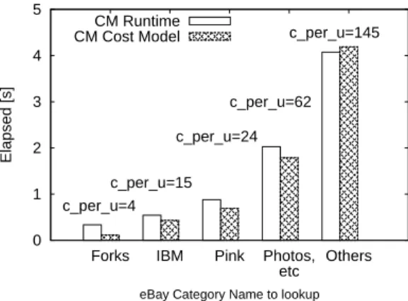
Experiment 4: In this experiment, we demonstrate that our cost model based on c per u captures actual query costs accurately. The data set and clustered key used in this experiment are the same as in Experiment 1, but we use a different query shown below which has a predicate on CAT5:
SELECT AVG(Price) FROM ITEMS WHERE CAT5=X
In other words, we select over a particular subcategory in the fifth level of the eBay product hierarchy. We build a CM on CAT5, which is strongly correlated with CATID. We tested different values chosen from the CAT5 category that exhibited different c per u counts (ranging from 4 to 145). Our cost model predicts that the CM’s performance is primarily determined by how many clustered attribute values the predicated unclustered value corresponds to. As Figure 10 shows, this cost model effectively captures the performance of a CM with various c per u values.
Experiment 5: For our final experiment, we use the SDSS dataset to demonstrate a situation where composite CMs have an advantage over single-attribute CMs as well as secondary B+Tree indexes with a real-world query. This is an example of a non-trivial correlation that was discovered by our CM Advisor tool. The clustered attribute objID is correlated strongly with the pair (ra, dec), but the correlation is weaker with each individual attribute. We use the following query, a variant of Q2 from SDSS that identifies objects having blue and bright surfaces within a region.
SELECT COUNT(*) FROM PhotoTag WHERE ra BETWEEN 193.117 AND 194.517
![Table 3: Clustered attribute bucketing granularity and I/O cost Bucket Size [pgs / bucket] Pages Scanned IO Cost [ms]](https://thumb-eu.123doks.com/thumbv2/123doknet/14498478.527397/9.918.93.420.84.187/table-clustered-attribute-bucketing-granularity-bucket-bucket-scanned.webp)