HAL Id: hal-02418404
https://hal.inria.fr/hal-02418404
Submitted on 18 Dec 2019
HAL is a multi-disciplinary open access
archive for the deposit and dissemination of
sci-entific research documents, whether they are
pub-lished or not. The documents may come from
teaching and research institutions in France or
abroad, or from public or private research centers.
L’archive ouverte pluridisciplinaire HAL, est
destinée au dépôt et à la diffusion de documents
scientifiques de niveau recherche, publiés ou non,
émanant des établissements d’enseignement et de
recherche français ou étrangers, des laboratoires
publics ou privés.
Numerical investigation of Landau damping in
dynamical Lorentz gases
Thierry Goudon, Léo Vivion
To cite this version:
Thierry Goudon, Léo Vivion. Numerical investigation of Landau damping in dynamical Lorentz gases.
Physica D: Nonlinear Phenomena, Elsevier, 2019. �hal-02418404�
Numerical investigation of Landau damping in dynamical Lorentz
gases
Thierry
Goudon
a,∗,
Léo
Vivion
aaUniversité Côte d’Azur, Inria, CNRS, LJAD, Parc Valrose, F-06108 Nice, France
A R T I C L E I N F O
Keywords:
Vlasov–like equations Interacting particles Landau damping Inelastic Lorentz gas
Finite elements and semi-Lagrangian schemes
A B S T R A C T
We investigate numerically the behavior of a particle, or a set of particles, which exchange momentum and energy with the environment, described as a transverse vibrational field. The large time behavior is characterized, in some specific circumstances, by means of effective friction force and Landau damping. In order to discuss these issues on numerical grounds, we set up a dedicated numerical method. The scheme couples a Finite Element Method for the wave equation, with an appropriate transparent boundary condition that preserves the dispersive effects driving the asymptotic behavior of the system, and a symplectic scheme or a Semi-Lagrangian method for the evolution of the particles. The time discretisation is constructed to capture accurately the energy exchanges. The numerical simulations shed new light on the theoretical results and bring out clearly the role of the parameters of the models.
1. Introduction
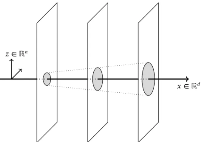
This paper is devoted to the numerical investigation of equations modeling the interaction of particles with their en-vironment, according to a description originally introduced by L. Bruneau & S. de Bièvre [5]. We refer the reader to Fig.1for a rough picture that can guide the intuition on this description. Particles evolve in the physical space ℝ𝑑, and
the behavior of the environment is embodied into a vibra-tion field which waves in the transverse direcvibra-tion ℝ𝑛. The
motion space and the vibration space are distincts and there is no a priori relation between 𝑛 and 𝑑. The environment can be thought of as a (continuum) set of membranes, activated by the passage of the particles, as depicted in Fig.1, and on each position 𝑥 ∈ ℝ𝑑, the particles can exchange
momen-tum and energy with the membranes.
𝑥∈ ℝ𝑑
𝑧∈ ℝ𝑛
Figure 1: Particle-wave interactions
The interaction is thus driven by the following
parame-∗Corresponding author
thierry.goudon@inria.fr(T. Goudon);leo.vivion@unice.fr(L. Vivion)
ORCID(s):
ters:
• two form functions 𝑥 ∈ ℝ𝑑 ↦ 𝜎
1(𝑥)and 𝑧 ∈ ℝ𝑛↦
𝜎2(𝑧)determine the interaction domain, in the physi-cal and the transverse directions respectively, between the particles and the waves; they are both non nega-tive, spherically symmetric, infinitely smooth and com-pactly supported;
• the vibration field is characterized by the (uniform) wave speed 𝑐 > 0.
As we shall see below, the dimension 𝑛 of the vibrational direction plays also a fundamental role.
The behavior of a single particle governed by this dy-namics is discussed in [5]: with 𝑞(𝑡) denoting the position of the particle, and 𝜓(𝑡, 𝑥, 𝑧) describing the environment, one considers the system
̈ 𝑞(𝑡) = −∇𝑊 (𝑞(𝑡)) (1a) − ∬ℝ𝑑×ℝ𝑛 𝜎1(𝑞(𝑡) − 𝑦)𝜎2(𝑧)∇𝑦𝜓(𝑡, 𝑦, 𝑧) d𝑦 d𝑧, 𝜕𝑡𝑡2𝜓− 𝑐2Δ𝑧𝜓= −𝜎2(𝑧)𝜎1(𝑥 − 𝑞(𝑡)), (1b) for 𝑡 ≥ 0, 𝑥 ∈ ℝ𝑑, 𝑧 ∈ ℝ𝑛. Equation (1a) also takes into
account the effect of an external potential 𝑥 ↦ 𝑊 (𝑥). The system (1a)–(1b) is completed by initial data
(𝑞(0), ̇𝑞(0)) = (𝑞0, 𝑝0),
(𝜓(0, 𝑥, 𝑧), 𝜕𝑡𝜓(0, 𝑥, 𝑧)) = (𝜓0(𝑥, 𝑧), 𝜓1(𝑥, 𝑧)). (2) A fundamental feature of the model is the conservation of the total energy. Let
𝐸particle(𝑡) = 1 2 ̇𝑞(𝑡) 2 + 𝑊 (𝑞(𝑡)) + ∬ℝ𝑑×ℝ𝑛 𝜎1(𝑞(𝑡) − 𝑦)𝜎2(𝑧)𝜓(𝑡, 𝑦, 𝑧) d𝑦 d𝑧 (3)
and 𝐸wave(𝑡) = 1 2∬ℝ𝑑×ℝ𝑛||𝜕𝑡 𝜓(𝑡, 𝑥, 𝑧)||2 d𝑥 d𝑧 +𝑐 2 2 ∬ℝ𝑑×ℝ𝑛||∇𝑧 𝜓(𝑡, 𝑥, 𝑧)||2 d𝑥 d𝑧. (4) Then, we have 𝐸(𝑡) = 𝐸particle(𝑡) + 𝐸wave(𝑡) = 𝐸(0). (5) As time becomes large, the remarkable fact brought out in [5] is that the membranes eventually act as a friction force on the particle. To be more specific, the flavor of the large time asymptotics of the particle can be recapped in the following statement (for precise statements and detailed assumptions, we refer the reader to [5, Theorems 2 & 4]).
Theorem 1. Let 𝑛 = 3. For any 𝜂 ∈ (0, 1) there exists a
critical wave speed 𝑐0 = 𝑐0(𝜂) > 0and constants 𝛾, 𝐾 > 0
(which do not depend on 𝜂) such that the following assertions hold
• Constant force, [5, Theorem 2]: if 𝑊 (𝑥) = ⋅ 𝑥 for a certain ∈ ℝ𝑑constant and small enough compared
to 𝑐−1, then, there exists 𝑞
∞ ∈ ℝ𝑑 and 𝑣() ∈ ℝ𝑑
such that, for any 𝑐 ≥ 𝑐0, we have ||𝑞∞+ 𝑡 𝑣() − 𝑞(𝑡)|| ≤ 𝐾𝑒
−𝛾(1−𝜂) 𝑐3 𝑡;
• Confining potential, [5, Theorem 4]: if 𝑊 (𝑥) →|𝑥|→+∞
+∞, then as time tends to ∞, ̇𝑞(𝑡) converges to 0 and
𝑞(𝑡)converges to a critical point 𝑞⋆ of the potential
𝑊. If 𝑞⋆is a non degenerate minimum of 𝑊 , then,
for any 𝑐 ≥ 𝑐0, we have ||𝑞(𝑡) − 𝑞⋆|| ≤ 𝐾𝑒−𝛾(1−𝜂)2𝑐3 𝑡.
Remark 2. The following comments are worthwhile:
• We point out the role of the assumptions “the wave speed 𝑐 is large enough” and on the dimension 𝑛 for the wave propagation. That 𝑐 is large can be inter-preted as a condition ensuring that the energy is quickly evacuated in the membrane, when the particle hits this membrane. The following two intuitive arguments for choosing the dimension 𝑛 = 3 can be given: first, it en-sures a strong enough dispersion effect, which would be too weak in lower dimensions; second, the Huy-gens principle implies that the energy transferred to the membrane is really evacuated and cannot be felt at the hitting point after a while.
• When the particle is subjected to a constant external force, asymptotically as time becomes large it has a uniform rectilinear motion. Assuming 𝑛 = 3 also al-lows us to identify the asymptotic action of the vibra-tions as a friction force proportional to the velocity of the particle (see [5, Eq. (2.9)]).
• When the particle is subjected to a confining poten-tial, it stops exponentially fast at a critical point of the potential.
This statement tells us that, in certain circumstances, the interaction with the environment acts on the particle as a drag force: the large time behavior looks like the one of the system
̇𝑞(𝑡) = 𝑝(𝑡), ̇𝑝(𝑡) = −∇𝑊 (𝑞(𝑡)) − 𝜆𝑝(𝑡),
with an effective friction coefficient 𝜆 > 0. This is precisely the motivation presented in [5] to shed some light on the conditions driving to such a friction effect, by coming back to a more microscopic and detailed description of the inter-action, that takes into account the dynamics of the environ-ment, here represented by a scalar vibration field.
Therefore, this work fits in the framework of open sys-tems theory where a classical, or quantum, system is cou-pled to its environment through exchanges of mass, momen-tum or energy. In turn, the environment has a dissipative action on the system, an idea that dates back to the seminal works of Caldeira-Leggett [6,7]. We refer the reader to [27] for an overview on such models for classical particles, and the presentation of a quite general framework that encom-passes many physical situations of interest. In particular, it is worth mentioning the related attempts to model frictional damping from the interaction with a wave field coupled to the moving particle [25,26] and [19], where the environ-ment is described as a Bose gas, and the slowing down of the particle is interpreted in terms of Cherenkov radiation effects. The originality of the model introduced in [5] is to model the environment as a vibrational field that can evac-uate energy in directions transverse to the particle’s motion. Then, the wish is to derive an effective formula, depend-ing on the interaction parameters (here 𝜎1, 𝜎2, 𝑐...) for the drag coefficient 𝜆. One also expects, for small applied force , that the limiting velocity 𝑣() becomes proportional to the force: 𝑣() ∼→0 𝜇, in the spirit of Ohm’s law, and one is interested in identifying the corresponding mobility
𝜇. Complementary studies of the model (1a)–(1b) can be
found in [1,11,12,13,27,32], with connections to stochas-tic homogenization and to the classical Lorentz problems. We also refer to [8] for a quantum version of the model, and further connection to the Cherenkov radiation.
It is natural to extend the model (1a)–(1b) by considering a set of 𝑁 particles which all interact with the membranes. Let 𝑞𝑖stand for the position of the 𝑖th particle. The system
is now governed by the system
̈ 𝑞𝑖(𝑡) = −∇𝑊 (𝑞𝑖(𝑡)) (6a) − ∬ℝ𝑑×ℝ𝑛 𝜎1(𝑞𝑖(𝑡) − 𝑦)𝜎2(𝑧)∇𝑦𝜓(𝑡, 𝑦, 𝑧) d𝑦 d𝑧, (6b) 𝜕𝑡𝑡2𝜓− 𝑐2Δ𝑧𝜓= −𝜎2(𝑧) (𝑁 ∑ 𝑖=1 𝜎1(𝑥 − 𝑞𝑖(𝑡)) ) , (6c)
for 𝑡 ≥ 0, 𝑥 ∈ ℝ𝑑, 𝑧 ∈ ℝ𝑛. Considering the mean field
𝑁 →∞, assuming that the strength of the force on a given particle scales like 1∕𝑁), one is led to a kinetic equation
𝜕𝑡𝐹+ 𝑣⋅ ∇𝑥𝐹 (7a) − ∇𝑥 ( 𝑊 + 𝜎1⋆𝑥 ∫ 𝜎2𝜓d𝑧 ) ⋅ ∇𝑣𝐹 = 0, 𝜕𝑡𝑡2𝜓− 𝑐2Δ𝑧𝜓= −𝜎2(𝑧) ( 𝜎1⋆𝑥 ∫ 𝐹d𝑣 ) , (7b)
for 𝑡 ≥ 0, 𝑥 ∈ ℝ𝑑, 𝑣 ∈ ℝ𝑑, 𝑧 ∈ ℝ𝑛, where the unknown 𝐹
stands for the particles distribution function in phase space, see [21]. These systems still satisfy the energy conservation property (5), just adapting the definition of the energy asso-ciated to the particles as follows:
𝐸particles(𝑡) = 𝑁 ∑ 𝑖=1 (1 2 ̇𝑞𝑖(𝑡) 2 + 𝑊 (𝑞𝑖(𝑡)) + ∬ℝ𝑑×ℝ𝑛 𝜎1(𝑞𝑖(𝑡) − 𝑦)𝜎2(𝑧)𝜓(𝑡, 𝑦, 𝑧) d𝑦 d𝑧 ) (8) for (6a)–(6c) and 𝐸particles(𝑡) = ∬ℝ𝑑×ℝ𝑑 𝐹(𝑡, 𝑥, 𝑣) ( 𝑣2 2 + 𝑊 (𝑥) + ∬ℝ𝑑×ℝ𝑛 𝜎1(𝑥 − 𝑦)𝜎2(𝑧)𝜓(𝑡, 𝑦, 𝑧) d𝑦 d𝑧 ) d𝑥 d𝑣 (9) for (7a)–(7b). We refer the reader to [9] for the well-posedness analysis of the Vlasov-Wave system (7a)–(7b). As a matter of fact, we point out that 𝐹 naturally remains non-negative, all 𝐿𝑝 (1 ≤ 𝑝 ≤ +∞) norms are conserved as well as the
entropy functional
𝐻(𝑡) =
∬ℝ𝑑×ℝ𝑑
𝐹(𝑡) log(𝐹 (𝑡)) d𝑥 d𝑣.
More generally, for any 𝐴 ∶ ℝ+→ ℝthe integral (Casimir functionals)
∬ℝ𝑑×ℝ𝑑
𝐴(𝐹 (𝑡)) d𝑥 d𝑣
is conserved. These fundamental properties are consequences of the fact that the flow
𝜑𝑡∶ (𝑥0, 𝑣0) ↦ (𝒳 (𝑡), 𝒱 (𝑡)) defined by the ODE system
d d𝑡𝒳 (𝑡) = 𝒱 (𝑡), d d𝑡𝒱 (𝑡) = −∇𝑥𝑊(𝒳 (𝑡)) − ∇𝑥𝜙(𝑡,𝒳 (𝑡)), 𝒳 (0) = 𝑥0, 𝒱 (0) = 𝑣0 (10) where 𝜙(𝑡, 𝑥) = ∬ℝ𝑑×ℝ𝑛 𝜎1(𝑥 − 𝑦)𝜎2(𝑧)𝜓(𝑡, 𝑥, 𝑧) d𝑧 d𝑦, (11)
is symplectic. Indeed, denoting
𝐽 = ( 0𝑑 𝐼𝑑 −𝐼𝑑 0𝑑 ) , we have (Jac 𝜑𝑡)𝑇𝐽(Jac 𝜑𝑡) = 𝐽 .
In particular, det(Jac 𝜑𝑡)2 = 1and volumes are conserved
by the flow. We deduce the asserted conservation properties since the distribution function 𝐹 is constant along the flow
𝜑𝑡: for any 𝑡 ≥ 0, 𝐹 (𝑡, 𝑥, 𝑣) = 𝐹0(𝜑−𝑡(𝑥, 𝑣)).
Remark 3. The construction of the numerical method will
use this property, which equally applies to the particulate systems as follows. Given a solution of (1a)–(1b), associated
to the initial data (𝑞0, 𝑝0,Ψ0,Ψ1), we have at hand the
poten-tial defined by the formula (11), and it makes sense to
con-sider the differential system (10) (where a priori (𝑥0, 𝑣0) ≠ (𝑞0, 𝑝0); when the equality holds the trajectories coincide (𝑞(𝑡), 𝑝(𝑡)) = (𝒳 (𝑡), 𝒱 (𝑡))). It describes the motion of a
“fic-titious particle”, governed by the potential 𝜙. This system is still symplectic. A similar conclusion applies when starting from (6a)–(6c). However, we warn the reader not to be
con-fused: the differential system (1a)–(1b), or (6a)–(6c), itself
is by no means symplectic (which would be contradictory with Theorem1and the numerical experiments). This ob-servation will be crucial for the construction of the numeri-cal scheme: on a given time step, one has to solve the ODE system with 𝜓 considered as given, which motivates the use of a symplectic method in order to preserve accurately the energetic properties of the model.
Remark 4. Contrarily to a common practice, we have
in-corporated the interaction potential in definition (3), and its
counterparts for the many-particles frameworks. It is seen as the potential exerted by the wave on the particle, consis-tently with the viewpoint developed in [9]. This formulation will be also natural for discussing the numerical strategy and the preservation of the energy exchanges.
One might wonder what the friction effect observed on a single particle becomes when one deals with a large number of particles, either with the discrete model (6a)–(6c) or the kinetic model (7a)–(7b). Surprisingly, the conclusion might substantially differ (see also the recent results in [35] which gives interesting hints on the large time behavior for the 𝑁 particles system and comments on the loss of convergence rate in mean field regime 𝑁 → ∞). In fact the analysis per-formed in [9] establishes an unexpected connection between (7a)–(7b) and the attractive Vlasov–Poisson system, which can be obtained in a certain asymptotic regime as 𝑐 → ∞. In the same spirit, several stationary solutions of (7a)–(7b) can be identified, by means of free energy minimization, and their stability has been established [10]. Moreover, still based on the analogies with the Vlasov-Poisson system, it has been shown that the Vlasov-Wave system (7a)–(7b) can lead to a Landau damping effect, as summarized in the fol-lowing statement (see [22] for further details).
Theorem 5. Let 𝑊 = 0, 𝑛 = 3 and suppose that 𝑥 ∈ 𝕋𝑑. If
the initial data (𝐹0, 𝜓0, 𝜓1)are homogeneous with respect to
𝑥, then the unique solution (𝐹 (𝑡), 𝜓(𝑡)) of (7a)–(7b) satisfies 𝐹(𝑡) = 𝐹0 for any 𝑡. If 𝐹0 satisfies a certain criterion of
linear stability and considering ( ̃𝐹0, ̃𝜓0, ̃𝜓1)small enough
perturbations of (𝐹0, 𝜓0, 𝜓1), then, the associated solution ( ̃𝐹(𝑡), ̃𝜓(𝑡))of (7a)–(7b) satisfies the following properties:
• the force term
−∇𝑥 (
𝜎1⋆𝑥∫ 𝜎2𝜓̃d𝑧 )
converges (strongly) to 0,
• if, moreover, ̃𝐹0has the same mass as 𝐹0, the macro-scopic density ∫ ̃𝐹d𝑣converges (strongly) to ∫ 𝐹0d𝑣.
Remark 6. Let us make the following comments:
• The analysis follows arguments for the Vlasov-Poisson system, see [28] and [3]; it adapts also when deal-ing for the problem set on ℝ𝑑, following [4]. The
de-cay rate can be explicited, depending on the functional framework for the perturbation ̃𝐹0.
• Given a spatially homogeneous profile 𝐹0, the
crite-rion ensuring the linear stability holds provided 𝑐 is large enough.
• Again, the role of the dimension 𝑛 = 3 (in fact 𝑛 odd and 𝑛 ≥ 3) is crucial for establishing the Landau damping.
We wish to investigate these questions on numerical grou-nds. In particular, we address the following issues:
• for the single particle model (1a)–(1b), to illustrate the validity of Theorem1and observe the friction effect, for both a confining potential or a constant force, in which case we discuss the behavior of the asymptotic speed.
• for (6a)–(6c), to investigate the 𝑁-particles large time dynamics. When 𝑁 > 1 particles interact, the situ-ation looks much more intricate and several scenario emerge. Roughly speaking either the particles ignore each other, possibly after a very short time of interac-tion, and they behave as they were alone, or they form clusters that create their own confining potential. Such cluster may move or stop, even if, individually, each particle in the cluster keeps moving. (Further results on the large time asymptotics for 𝑁 particles in a con-fining potential can be found in [35].)
• For the kinetic model (7a)–(7b), to illustrate the Lan-dau damping phenomena.
We will pay a specific attention to discuss the role of the as-sumptions of the space dimension 𝑛, and on the wave-speed 𝑐. The numerical investigation of these questions re-quire to take into consideration the specific features of the models in order to construct the numerical method:
• as said above, the friction/damping phenomena de-pend on the wave-space dimension 𝑛, and the case
𝑛 = 3definitely has a specific role. Moreover, these phenomena are, more or less, related to the ability to evacuate the energy through the membranes. Hence, one has to simulate the free space wave equation, in dimension 𝑛 = 3. This requires to pay attention to the conditions imposed at the boundaries of the wave-computational domain, in order not to perturb the ne-cessary dispersion effects, which are essential for the asymptotic properties.
• the energy balance, and in particular the exchanges be-tween the kinetic energy of the particles and the vi-brational energy of the membranes, are also crucial features of the models, and the discrete version of the problem should preserve as far as possible the dynam-ics of these exchanges.
These considerations will guide the technical choices to de-sign the numerical scheme. The paper is organized as fol-lows. In Section2, we describe how we can take advantage of spherical symmetries to set up transparent boundary con-ditions for the wave equation in dimension 𝑛 = 3. Sections3
and 4are devoted to the discretization of the equations, in the 𝑁 particles and in the kinetic frameworks, respectively. In Section5, we discuss in details the energetic properties of the schemes. We present the numerical results in Section6.
2. Discretization of the wave equation with a
transparent boundary condition
In dimension 𝑛 = 1, the wave equation propagates the information to the right and to the left with velocities ±𝑐, and considering the expression of the solution given by D’Alem-bert’s formula, we find that
(𝜕𝑡+ 𝑐𝜕𝑥)𝜓(𝑡, 𝑅max) = 0 = (𝜕𝑡− 𝑐𝜕𝑥)𝜓(𝑡, −𝑅max) constitues transparent boundary conditions that can be used when truncating the computational domain to the interval (−𝑅max,+𝑅max). Furthermore, these conditions can be eas-ily implemented. Unfortunately, finding relevant boundary conditions in higher dimensions is far more challenging and leads to non local formula, see [14]. Nevertheless, in the par-ticular case of the dimension 𝑛 = 3 (note that Theorems1
and5use this assumption) and for radially symmetric data, there exists a transformation that allows us to go back to the classical wave equation in dimension 𝑛 = 1, see e.g. [36].
2.1. Radially symmetric wave equation
Consider the wave equation in dimension 𝑛 = 3
𝜕𝑡𝑡2𝜓− 𝑐2Δ𝑧𝜓= −𝜎2(𝑧) 𝑆(𝑡, 𝑥). (12) We suppose that
𝜎2(𝑧) = ̃𝜎2(|𝑧|)
is radially symmetric. If, furthermore, the initial condition (𝜓0(𝑥, 𝑧), 𝜓1(𝑥, 𝑧)) = (Ψ0(𝑥,|𝑧|), Ψ1(𝑥,|𝑧|))
is radially symmetric too, then the unique solution 𝜓 of (12) is radially symmetric. We have 𝜓(𝑡, 𝑥, 𝑧) = Ψ(𝑡, 𝑥, |𝑧|) and Ψsatisfies 𝜕𝑡𝑡2Ψ − 𝑐2 ( 𝜕2𝑟𝑟Ψ +𝑛− 1 𝑟 𝜕𝑟Ψ ) = − ̃𝜎2(𝑟)𝑆(𝑡, 𝑥). We set 𝑢(𝑡, 𝑥, 𝑟) = 𝑟Ψ(𝑡, 𝑥, 𝑟). (13) Using that 𝑛 = 3, we check that 𝑢 is a solution of the classical wave equation in dimension one
𝜕𝑡𝑡2𝑢−𝑐2𝜕𝑟𝑟2𝑢= 𝑟(𝜕𝑡𝑡2Ψ − 𝑐2𝜕𝑟𝑟2Ψ − 𝑐22
𝑟𝜕𝑟Ψ
)
= −𝑟 ̃𝜎2(𝑟)𝑆(𝑡, 𝑥). Therefore, truncating the domain to |𝑧| ≤ 𝑅max, we can use
𝜕𝑡𝑢+ 𝑐𝜕𝑟𝑢= 0
as a (simple and exact) transparent boundary condition for
𝑟 = 𝑅max. Eventually, we have to solve numerically the following system, for 𝑡 ≥ 0 and 0 < 𝑟 < 𝑅max,
𝜕𝑡𝑡2𝑢− 𝑐2𝜕𝑟𝑟2𝑢= −𝑟 ̃𝜎2(𝑟)𝑆(𝑡, 𝑥), (14a) (𝑢(0, 𝑥, 𝑟), 𝜕𝑡𝑢(0, 𝑥, 𝑟)) = (𝑟Ψ0(𝑥, 𝑟), 𝑟Ψ1(𝑥, 𝑟)), (14b)
𝑢(𝑡, 𝑥, 0) = 0, 𝜕𝑡𝑢(𝑡, 𝑥, 𝑅max) + 𝑐𝜕𝑟𝑢(𝑡, 𝑥, 𝑅max) = 0. (14c) We remind the reader that 𝑥 appears here as a parameter. In practice, we shall discretize the physical space, and thus we shall deal with this system for a finite number of grid points
𝑥. Once 𝑢 determined by solving (14a)–(14c), we can come
back to the original unknown Ψ (and then 𝜓): for any 𝑟 ≠ 0, we have Ψ(𝑡, 𝑥, 𝑟) = 𝑢(𝑡, 𝑥, 𝑟)∕𝑟 and for 𝑟 = 0, we derive (13) to get
𝜕𝑟𝑢(𝑡, 𝑥, 𝑟) = Ψ(𝑡, 𝑥, 𝑟) + 𝑟𝜕𝑟Ψ(𝑡, 𝑥, 𝑟).
Since for any smooth solution of (12), 𝜕𝑟Ψ(𝑡, 𝑥, 0)is bounded
(in fact for these solutions 𝜕𝑟Ψ(𝑡, 𝑥, 0) = 0), we eventually
get Ψ(𝑡, 𝑥, 0) = 𝜕𝑟𝑢(𝑡, 𝑥, 0). Nevertheless, for our purposes,
it is not necessary to reconstruct 𝜓 to solve (1a), (6a) or (7a). Indeed, for these three equations we can write the potential
𝜙(𝑡, 𝑥) = ∬ℝ𝑑×ℝ𝑛 𝜎1(𝑥 − 𝑦)𝜎2(𝑧)𝜓(𝑡, 𝑦, 𝑧) d𝑦 d𝑧 by means of 𝑢: 𝜙(𝑡, 𝑥) = 4𝜋 ∫ℝ𝑑 𝜎1(𝑥−𝑦) ( ∫ 𝑅max 0 𝑟 ̃𝜎2(𝑟)𝑢(𝑡, 𝑦, 𝑟) d𝑟 ) d𝑦. (15) This equality (15) holds true as far as
supp( ̃𝜎2) ⊂ [0, 𝑅max],
a condition that we shall use to choose the cut-off parameter
𝑅max.
2.2. Discretization of the radial wave equation
(
14a
)–(
14c
).
Let us explain the discretization method for the wave equation; we use quite classical approaches and further in-formation about the schemes can be found in e. g. [2,37].
Radial discretization. We use a Finite Element Method
(FEM). To this end, we introduce a subdivision 0 = 𝑟1< 𝑟2< .... < 𝑟𝐾= 𝑅max
of [0, 𝑅max]and a basis (𝜑1, ..., 𝜑𝐾)(with 𝐾 ≥ 𝐾) of
polynomial functions associated to this partition and the choice of the family of finite elements. The approached solution reads 𝑢ℎ(𝑡, 𝑥, 𝑟) =
∑𝐾
𝑘=1𝑢𝑘(𝑡, 𝑥)𝜑𝑘(𝑟)where the numerical unknowns are collected in 𝑈(𝑡, 𝑥) = (𝑢1, ..., 𝑢𝐾)(𝑡, 𝑥), the
vector determined by the system d
2
d𝑡2𝑈(𝑡, 𝑥) + d
d𝑡𝑈(𝑡, 𝑥) +𝑈 (𝑡, 𝑥) = 𝐺(𝑡, 𝑥). (16) In (16), is the mass matrix, the diffusion matrix, the rigidity matrix and the components of 𝐺(𝑡, 𝑥) are given by
−𝑆(𝑡, 𝑥) ∫
𝑅max
0
𝑟 ̃𝜎2(𝑟)𝜑𝑘(𝑟) d𝑟, for 𝑘 ∈ {1, ..., 𝐾}.
Note that Dirichlet boundary conditions are encoded in the mass matrix whereas the transparent boundary condition is encoded in the diffusion matrix .
Time discretization.Next, we make use of Newmark scheme
for treating the time derivatives in (16). Let 𝛿𝑡 > 0 stand for the time step and set 𝑡𝑛 = 𝑛𝛿𝑡. Then, the approximation of
the solution 𝑢 at time 𝑡𝑛is 𝑢𝑛(𝑥, 𝑟) =∑𝐾 𝑘=1𝑢
𝑛
𝑘(𝑥)𝜑𝑘(𝑟). We
denote 𝑈𝑛
𝑥 the vector with components 𝑢 𝑛
𝑘(𝑥). For 𝐺(𝑡, 𝑥) =
0, the Newmark scheme reads
𝑈 𝑛+1 𝑥 − 2𝑈𝑥𝑛+ 𝑈𝑛 −1 𝑥 𝛿𝑡2 +𝑑 𝑈 𝑛+1 𝑥 + (1 − 2𝑑)𝑈𝑥𝑛+ (𝑑 − 1)𝑈𝑥𝑛−1 𝛿𝑡 +(𝜃 𝑈𝑥𝑛+1+ (1∕2 + 𝑑 − 2𝜃)𝑈𝑥𝑛 +(1∕2 − 𝑑 + 𝜃)𝑈𝑥𝑛−1)= 0 (17) where 0 ≤ 𝑑 ≤ 1 and 0 ≤ 𝜃 ≤ 1∕2 are parameters of the scheme. Of course, in our situation, 𝐺(𝑡, 𝑥) ≠ 0 and the choice of the time discretization of 𝐺 will depend on the cou-pling with (1a) (resp. (6a) or (7a)). This will be detailed later on. In practice we will only use this scheme with (𝑑, 𝜃) = (1∕2, 1∕4). For these parameters the scheme is second order accurate in time and 𝑘th order in space, where 𝑘 depends of the choice of the FEM basis. Moreover, for these parameters, as far as the support of the wave remains included in the com-putational domain, the scheme conserves the discrete energy of the homogeneous wave equation. More precisely, as far as 𝑈𝑚
⟨ 𝑈 𝑛+1 𝑥 − 𝑈 𝑛 𝑥 Δ𝑡∕2 , 𝑈𝑥𝑛+1− 𝑈𝑥𝑛 Δ𝑡∕2 ⟩ + ⟨ 𝑈 𝑛+1 𝑥 + 𝑈 𝑛 𝑥 2 , 𝑈𝑥𝑛+1+ 𝑈𝑥𝑛 2 ⟩ = ⟨ 𝑈 𝑛 𝑥− 𝑈 𝑛−1 𝑥 Δ𝑡∕2 , 𝑈𝑥𝑛− 𝑈𝑥𝑛−1 Δ𝑡∕2 ⟩ + ⟨ 𝑈 𝑛 𝑥+ 𝑈 𝑛−1 𝑥 2 , 𝑈𝑥𝑛+ 𝑈𝑥𝑛−1 2 ⟩ . (18)
3. Discretization of
(
1a
)–(
1b
)
We restrict ourselves to the case where the particles evolve in the one-dimensional torus: 𝑑 = 1 and 𝑥 ∈ 𝕋𝐿∶= ℝ∕(𝐿ℤ)
(where 𝐿 > 0). For (1a), we thus impose 𝑞(𝑡) ∈ 𝕋𝐿. Then
we are led to discretize the following system ⎧ ⎪ ⎨ ⎪ ⎩ ̇𝑞(𝑡) = 𝑝(𝑡), ̇𝑝(𝑡) = −𝜕𝑥𝑊(𝑞(𝑡)) − 𝜕𝑥𝜙(𝑡, 𝑞(𝑡)), (𝑞(0), ̇𝑞(0)) = (𝑞0, 𝑝0), 𝑞(𝑡) ∈ 𝕋𝐿, coupled to ⎧ ⎪ ⎪ ⎨ ⎪ ⎪ ⎩ 𝜕𝑡𝑡2𝑢− 𝑐2𝜕𝑟𝑟2𝑢= −𝑟 ̃𝜎2(𝑟)𝜎1(𝑥 − 𝑞(𝑡)), (𝑢(0, 𝑥, 𝑟), 𝜕𝑡𝑢(0, 𝑥, 𝑟)) = (𝑟Ψ0(𝑥, 𝑟), 𝑟Ψ1(𝑥, 𝑟)), 𝑢(𝑡, 𝑥, 0) = 0, 𝜕𝑡𝑢(𝑡, 𝑥, 𝑅max) + 𝑐𝜕𝑟𝑢(𝑡, 𝑥, 𝑅max) = 0, where the potential 𝜙 is defined by (15).
As said in the previous section, we solve the wave equa-tion with a classical Newmark scheme with parameters (𝑑, 𝜃) = (1∕2, 1∕4). This ensures second order accuracy in time, and
𝑘th order with respect to the wave direction (depending on
the choice of the FEM; in practice we shall work with the Lagrange ℙ2 elements, which reaches second order accu-racy). The symplectic property of the flow is a fundamental feature of the model. Hence, we make use of the Stormer-Verlet scheme (see (23) below) which is a second order ac-curate symplectic scheme: the discrete flow 𝜑𝑛∶ (𝑞0, 𝑝0) ↦ (𝑞𝑛, 𝑝𝑛)is symplectic, where 𝑞𝑛and 𝑝𝑛stand for the
approx-imation of 𝑞 and 𝑝 at time 𝑡𝑛, respectively. Further details
about symplectic schemes can be found e. g. in [20, Sec-tion 1.3.2] and [24,31].
We are left with the question of handling the coupling between the two evolution equations. To this end, we pay at-tention to the energy exchanges. We have already introduced the subdivision (𝑟1, ..., 𝑟𝐾)and the basis functions (𝜑1, ..., 𝜑𝑘).
Let Δ𝑡 > 0 be the time step. We have set 𝑡𝑛= 𝑛Δ𝑡; we shall
also need
𝑡𝑛+1∕2= (𝑛 + 1∕2)Δ𝑡.
Next, we also define a subdivision of the physical domain 0 = 𝑥1< ... < 𝑥𝑖 = 𝑖Δ𝑥 < ... < 𝑥𝑁 = 𝐿
characterized by the (uniform) space step Δ𝑥. We denote [𝑥𝑖−1
2
, 𝑥
𝑖+1
2
]the cell centered at 𝑥𝑖. Therefore the numerical
unknowns for the wave equation are denoted 𝑢𝑛
𝑖,𝑘; they define
the following approximation 𝑢𝑛of the wave at time 𝑡𝑛
𝑢𝑛(𝑥, 𝑟) = 𝑁 ∑ 𝑖=1 𝑘 ∑ 𝑘=1 𝑢𝑛𝑖,𝑘𝟏[ 𝑥 𝑖−12,𝑥𝑖+12 ](𝑥)𝜑 𝑘(𝑟).
It is also convenient to introduce
𝑢𝑛𝑘(𝑥) = 𝑁 ∑ 𝑖=1 𝑢𝑛𝑖,𝑘𝟏[ 𝑥 𝑖−1 2 ,𝑥 𝑖+1 2 ](𝑥), so that 𝑢𝑛𝑖,𝑘 = 1 Δ𝑥∫ 𝑥 𝑖+12 𝑥 𝑖−1 2 𝑢𝑛𝑘(𝑥) d𝑥. We shall denote 𝑈𝑛 𝑥 and 𝑈 𝑛
𝑖 the vector in ℝ𝐾 with
compo-nents 𝑢𝑛
𝑘(𝑥)and 𝑢 𝑛
𝑖,𝑘, respectively. Hence, the potential 𝜙 at
time 𝑡𝑛can be approached by
𝜙𝑛(𝑥) = 4𝜋 ∫ 𝐿 0 𝜎1(𝑥 − 𝑦) ( ∫ 𝑅max 0 𝑟 ̃𝜎2(𝑟)𝑢𝑛(𝑦, 𝑟) d𝑟 ) d𝑦 = 4𝜋 𝑁 ∑ 𝑖=1 𝐾 ∑ 𝑘=1 𝑢𝑛𝑖,𝑘 ⎛ ⎜ ⎜ ⎝∫ 𝑥 𝑖+12 𝑥 𝑖−1 2 𝜎1(𝑥 − 𝑦) d𝑦 ⎞ ⎟ ⎟ ⎠ × ( ∫ 𝑅max 0 𝑟 ̃𝜎2(𝑟)𝜑𝑘(𝑟) d𝑟 ) . (19) Accordingly, we have (𝜕𝑥𝜙)𝑛(𝑥) = 𝜕𝑥𝜙𝑛(𝑥) = 4𝜋 𝑁 ∑ 𝑖=1 𝐾 ∑ 𝑘=1 𝑢𝑛𝑖,𝑘 ⎛ ⎜ ⎜ ⎝∫ 𝑥 𝑖+1 2 𝑥 𝑖−1 2 𝜕𝑥𝜎1(𝑥 − 𝑦) d𝑦 ⎞ ⎟ ⎟ ⎠ × ( ∫ 𝑅max 0 𝑟 ̃𝜎2(𝑟)𝜑𝑘(𝑟) d𝑟 ) = 4𝜋 𝑁 ∑ 𝑖=1 𝐾 ∑ 𝑘=1 𝑢𝑛𝑖,𝑘 ( −𝜎1(𝑥 − 𝑥𝑖+1 2 ) + 𝜎1(𝑥 − 𝑥𝑖−1 2 )) × ( ∫ 𝑅max 0 𝑟 ̃𝜎2(𝑟)𝜑𝑘(𝑟) d𝑟 ) . (20)
Having at hand the approximated quantity 𝑢𝑛+1
2, we define
similarly the approached potential at time 𝑡𝑛+1
2. Eventually, we set 𝜙𝑛+14 = 𝜙 𝑛+1 2 + 𝜙𝑛 2 et 𝜕𝑥𝜙 𝑛+1 4 = 𝜕𝑥𝜙 𝑛+1 2 + 𝜕 𝑥𝜙𝑛 2 .
Time-discretization. Suppose that we have computed 𝑞𝑛,
𝑝𝑛, 𝑢𝑛−1∕2 and 𝑢𝑛. We are going to update these
quanti-ties and define 𝑞𝑛+1, 𝑝𝑛+1∕2, 𝑝𝑛+1, 𝑢𝑛+1∕2and 𝑢𝑛+1. To this end, we solve numerically the following two equations on the time interval [𝑡𝑛, 𝑡𝑛+1].
{ 𝜕𝑡𝑡2𝑢− 𝑐2𝜕𝑟𝑟2𝑢= −𝑟 ̃𝜎2(𝑟) 𝜎1(𝑥 − 𝑞𝑛) 𝑢(𝑡𝑛−12) = 𝑢𝑛− 1 2; 𝑢(𝑡𝑛) = 𝑢𝑛 ⎧ ⎪ ⎨ ⎪ ⎩ ̇𝑞(𝑡) = 𝑝(𝑡) ̇𝑝(𝑡) = −𝜕𝑥𝑊(𝑞(𝑡)) − 𝜕𝑥𝜙𝑛 +3 4(𝑞(𝑡)) 𝑞(𝑡𝑛) = 𝑞𝑛; 𝑝(𝑡𝑛) = 𝑝𝑛
The approximation 𝑞𝑛allows us to compute an
approxima-tion of the right hand side of the wave equaapproxima-tion: 𝑟̃𝜎2(𝑟)𝜎1(𝑥−
𝑞𝑛), that can be used on all the interval [𝑡𝑛, 𝑡𝑛+1]. Then, we
compute 𝑢𝑛+1∕2and 𝑢𝑛+1by applying the Newmark scheme on two half time steps. More precisely, we apply (17) with
𝛿𝑡 = Δ𝑡∕2and we average over the cell (𝑥𝑖−1∕2, 𝑥𝑖+1∕2). It leads to the following scheme:
⎧ ⎪ ⎪ ⎪ ⎪ ⎪ ⎪ ⎨ ⎪ ⎪ ⎪ ⎪ ⎪ ⎪ ⎩ 𝑈 𝑛+1 2 𝑖 − 2𝑈 𝑛 𝑖 + 𝑈 𝑛−1 2 𝑖 (Δ𝑡∕2)2 + 𝑈𝑛+ 1 2 𝑖 + 𝑈 𝑛−1 2 𝑖 Δ𝑡∕2 + ( 1 4𝑈 𝑛+1 2 𝑖 + 1 2𝑈 𝑛 𝑖 + 1 4𝑈 𝑛−1 2 𝑖 ) = 𝐺𝑛𝑖 𝑈 𝑛+1 𝑖 − 2𝑈 𝑛+1 2 𝑖 + 𝑈 𝑛 𝑖 (Δ𝑡∕2)2 + 𝑈𝑖𝑛+1+ 𝑈𝑛 𝑖 Δ𝑡∕2 + ( 1 4𝑈 𝑛+1 𝑖 + 1 2𝑈 𝑛+1 2 𝑖 + 1 4𝑈 𝑛 𝑖 ) = 𝐺𝑛 𝑖 (21) where 𝐺𝑛
𝑖 stands for the vector in ℝ𝐾with components
− ⎛ ⎜ ⎜ ⎝ 1 Δ𝑥∫ 𝑥 𝑖+1 2 𝑥 𝑖−1 2 𝜎1(𝑥 − 𝑞𝑛) d𝑥 ⎞ ⎟ ⎟ ⎠ ( ∫ 𝑅max 0 𝑟 ̃𝜎2(𝑟)𝜑𝑘(𝑟) d𝑟 ) . (22) We turn to the equation for the particle. With the obtained approximations of 𝑢, we define 𝜕𝑥𝜙𝑛+1∕2, 𝜕𝑥𝜙𝑛+1and 𝜕𝑥𝜙𝑛+3∕4=
(𝜕𝑥𝜙𝑛+1∕2 + 𝜕𝑥𝜙𝑛+1)∕2. Then we use on all the interval
[𝑡𝑛, 𝑡𝑛+1] this approximation of the force term. Since the force term −𝜕𝑥𝑊(𝑥) − 𝜕𝑥𝜙𝑛+3∕4(𝑥)is constant in time,
ap-plying the Stormer-Verlet scheme eventually leads to the fol-lowing scheme: ⎧ ⎪ ⎪ ⎨ ⎪ ⎪ ⎩ 𝑝𝑛+12 = 𝑝𝑛−Δ𝑡 2 𝜕𝑥𝑊(𝑞 𝑛) −Δ𝑡 2 𝜕𝑥𝜙 𝑛+3 4(𝑞𝑛) 𝑞𝑛+1= 𝑞𝑛+ Δ𝑡 𝑝𝑛+12 𝑝𝑛+1= 𝑝𝑛+12 − Δ𝑡 2 𝜕𝑥𝑊(𝑞 𝑛+1) −Δ𝑡 2 𝜕𝑥𝜙 𝑛+3 4(𝑞𝑛+1). (23) The full scheme is obtained by combining (21) and (23). We will justify this time discretization in terms of energy bal-ance in Section5.
4. Discretization of
(
7a
)–(
7b
)
Again, we restrict the discussion to the case 𝑥 ∈ 𝕋𝐿.
Moreover we should also deal with a truncated velocity do-main [−𝑉max, 𝑉max], where 𝑉maxis chosen large enough so that it is reasonable to impose
𝐹(𝑡, 𝑥, −𝑉max) = 0 = 𝐹 (𝑡, 𝑥, 𝑉max),
considering initial data such that supp(𝐹0) ⊂ 𝕋𝐿×[−𝑉max, 𝑉max]. We are thus concerned with the simulation of (adding an external potential does not add any difficulty, and we take
𝑊 = 0in this presentation for the sake of clarity): ⎧ ⎪ ⎪ ⎨ ⎪ ⎪ ⎩ 𝜕𝑡𝐹+ 𝑣 𝜕𝑥𝐹 − 𝜕𝑥𝜙 𝜕𝑣𝐹 = 0 𝐹(0, 𝑥, 𝑣) = 𝐹0(𝑥, 𝑣) 𝐹(𝑡, 0, 𝑣) = 𝐹 (𝑡, 𝐿, 𝑣) 𝐹(𝑡, 𝑥, −𝑉𝑚𝑎𝑥) = 𝐹 (𝑡, 𝑥, 𝑉𝑚𝑎𝑥) = 0 ⎧ ⎪ ⎪ ⎨ ⎪ ⎪ ⎩ 𝜕𝑡𝑡2𝑢− 𝑐2𝜕𝑟𝑟2𝑢= −𝑟 ̃𝜎2(𝑟)𝜎1(𝑥 − 𝑞(𝑡)) (𝑢(0, 𝑥, 𝑟), 𝜕𝑡𝑢(0, 𝑥, 𝑟)) = (𝑟Ψ0(𝑥, 𝑟), 𝑟Ψ1(𝑥, 𝑟)) 𝑢(𝑡, 𝑥, 0) = 0 𝜕𝑡𝑢(𝑡, 𝑥, 𝑅max) + 𝑐𝜕𝑟𝑢(𝑡, 𝑥, 𝑅max) = 0 where the potential 𝜙 is defined by (15).
The wave equation is treated by using the Newmark sche-me and the FEM as described above. For the kinetic equa-tion, we use a Semi-Lagrangian finite volume scheme: the Positive and Flux Conservative (PFC) method that guaran-tees at the discrete level the conservation of mass, positivity of the solution and a maximum principle. Details and com-ments about this scheme can be found e. g. in [18,16,17] and the references therein. Note that other approaches, based on DG or WENO approximations could be used as well, see [23,29,30] for details on such approaches for Vlasov’s equa-tions.
We adapt the time discretization described for (1a)–(1b) in order to care of the energy balance. With the time step Δ𝑡 > 0we still denote 𝑡𝑛= 𝑛Δ𝑡and 𝑡𝑛+1∕2 = (𝑛 + 1∕2)Δ𝑡. We construct a grid of the phase space with space and ve-locity steps Δ𝑥 > 0 and Δ𝑣 > 0 respectively. Let 𝑥𝑖+1∕2 = (𝑖+1∕2)Δ𝑥, for 𝑖 ∈ {1, ..., 𝑁}, and 𝑣𝑗+1∕2= (𝑗+1∕2)Δ𝑣, for
𝑗 ∈ {−𝑀, ..., 𝑀}, with 𝑁Δ𝑥 = 𝐿 and 𝑀Δ𝑣 = 𝑉max. We denote by 𝐶𝑖,𝑗the cell [𝑥𝑖−1∕2, 𝑥𝑖+1∕2]×[𝑣𝑗−1∕2, 𝑣𝑗+1∕2], with center (𝑥𝑖, 𝑣𝑗). From the discrete quantities 𝑢𝑛𝑖,𝑘, we construct
the approximation (𝑥, 𝑟) ↦ 𝑢𝑛(𝑥, 𝑟)as above. The potential
𝜙𝑛and 𝜕𝑥𝜙𝑛are still defined by (19) and (20). From the
numerical unknowns 𝐹𝑛
𝑖,𝑗, we define the approximated
dis-tribution function 𝐹𝑛(𝑥, 𝑣) = 𝑁 ∑ 𝑖=1 𝑀 ∑ 𝑗=−𝑀 𝐹𝑖,𝑗𝑛𝟏𝐶 𝑖,𝑗(𝑥, 𝑣).
The macroscopic density 𝜌 at time 𝑡𝑛is thus given by 𝜌𝑛(𝑥) = ∫ 𝑉𝑚𝑎𝑥 −𝑉𝑚𝑎𝑥 𝐹ℎ(𝑡, 𝑥, 𝑣) d𝑣 = 𝑁 ∑ 𝑖=1 ( Δ𝑣 𝑀 ∑ 𝑗=−𝑀 𝐹𝑖,𝑗𝑛 ) 𝟏[ 𝑥 𝑖−1 2 ,𝑥 𝑖+1 2 ](𝑥). (24) The convolution 𝜎1⋆ 𝜌at time 𝑡𝑛becomes
(𝜎1⋆ 𝜌)𝑛(𝑥) = 𝜎1⋆ 𝜌𝑛(𝑥) = Δ𝑣 𝑁 ∑ 𝑖=1 𝑀 ∑ 𝑗=−𝑀 𝐹𝑖,𝑗𝑛 ( ∫ 𝑥 𝑖+1 2 𝑥 𝑖−1 2 𝜎1(𝑥 − 𝑦) d𝑦 ) . (25)
4.1. Time-discretisation
Knowing the approximations of 𝐹 and 𝑢 up to 𝑡𝑛, we
ob-tain the updated quantities 𝑢𝑛+1∕2, 𝑢𝑛+1and 𝐹𝑛+1by solving the following equations on [𝑡𝑛, 𝑡𝑛+1]:
{ 𝜕𝑡𝑡2𝑢− 𝑐2𝜕2 𝑟𝑟𝑢= −𝑟𝜎2(𝑟)(𝜎1⋆ 𝜌)𝑛, 𝑢(𝑡𝑛−12) = 𝑢𝑛− 1 2 ; 𝑢(𝑡𝑛) = 𝑢𝑛, { 𝜕𝑡𝐹 + 𝑣 𝜕𝑥𝐹 − 𝜕𝑥𝜙𝑛+34 𝜕 𝑣𝐹 = 0. 𝐹(𝑡𝑛) = 𝐹𝑛 With 𝐹𝑛we determine (𝜎
1⋆𝜌)𝑛, which is used to evaluate the source term for the wave equation. Iterating over two time-steps 𝛿𝑡 = Δ𝑡∕2 the Newmark scheme (17), we get 𝑢𝑛+1∕2 and 𝑢𝑛+1. To be specific, we have
⎧ ⎪ ⎪ ⎪ ⎪ ⎪ ⎪ ⎨ ⎪ ⎪ ⎪ ⎪ ⎪ ⎪ ⎩ 𝑈 𝑛+1 2 𝑖 − 2𝑈 𝑛 𝑖 + 𝑈 𝑛−1 2 𝑖 (Δ𝑡∕2)2 + 𝑈𝑛+ 1 2 𝑖 + 𝑈 𝑛−1 2 𝑖 Δ𝑡∕2 + ( 1 4𝑈 𝑛+1 2 𝑖 + 1 2𝑈 𝑛 𝑖 + 1 4𝑈 𝑛−1 2 𝑖 ) = 𝐺𝑛𝑖 𝑈 𝑛+1 𝑖 − 2𝑈 𝑛+1 2 𝑖 + 𝑈 𝑛 𝑖 (Δ𝑡∕2)2 + 𝑈𝑖𝑛+1+ 𝑈𝑛 𝑖 Δ𝑡∕2 + ( 1 4𝑈 𝑛+1 𝑖 + 1 2𝑈 𝑛+1 2 𝑖 + 1 4𝑈 𝑛 𝑖 ) = 𝐺𝑛 𝑖 (26) where 𝑈𝑛 𝑖 = (𝑢 𝑛 𝑖,1, ..., 𝑢 𝑛
𝑖,𝐾)and the components 𝐺 𝑛 𝑖,𝑘are de-fined by − ⎛ ⎜ ⎜ ⎝ 1 Δ𝑥∫ 𝑥 𝑖+1 2 𝑥 𝑖−1 2 (𝜎1⋆ 𝜌)𝑛(𝑥) d𝑥 ⎞ ⎟ ⎟ ⎠ ( ∫ 𝑅max 0 𝑟 ̃𝜎2(𝑟)𝜑𝑘(𝑟) d𝑟 ) . (27) Having disposed of the wave equation, we compute the force terms 𝜕𝑥𝜙𝑛+1∕2and 𝜕𝑥𝜙𝑛+1, as well as
𝜕𝑥𝜙𝑛+3∕4= 𝜕𝑥𝜙
𝑛+1∕2+ 𝜕 𝑥𝜙𝑛+1
2 .
Replacing the force by this constant quantity over the time interval, we obtain 𝐹𝑛+1by solving the corresponding Liou-ville equation with the PFC scheme.
4.2. Discretisation of the kinetic equation with the
PFC scheme
We start with the time-splitting { 𝜕𝑡𝐹⋆+ 𝑣 𝜕𝑥𝐹⋆= 0, 𝑡 ∈ [𝑡𝑛, 𝑡𝑛+1] 𝐹⋆(𝑡𝑛) = 𝐹 (𝑡𝑛) = 𝐹𝑛 { 𝜕𝑡𝐹⋆⋆− 𝜕𝑥𝜙𝑛+ 3 4 𝜕 𝑣𝐹⋆⋆= 0, 𝑡 ∈ [𝑡𝑛, 𝑡𝑛+1] 𝐹⋆⋆(𝑡𝑛) = 𝐹⋆(𝑡𝑛+1).
The consistency analysis of such time splitting methods with Landau damping is considered in [15]. The solutions of these equations at the final time 𝑡𝑛+1 are obtained by inte-grating along characteristics:
⎧ ⎪ ⎪ ⎨ ⎪ ⎪ ⎩ 𝐹⋆(𝑡𝑛+1, 𝑥, 𝑣) = 𝐹⋆(𝑡𝑛, 𝑋(𝑡𝑛, 𝑡𝑛+1, 𝑥, 𝑣), 𝑣) = 𝐹⋆(𝑡𝑛, 𝑥− Δ𝑡 𝑣, 𝑣), 𝐹⋆⋆(𝑡𝑛+1, 𝑥, 𝑣) = 𝐹⋆⋆(𝑡𝑛, 𝑥, 𝑉(𝑡𝑛, 𝑡𝑛+1, 𝑥, 𝑣)) = 𝐹⋆⋆(𝑡𝑛, 𝑥, 𝑣+ Δ𝑡 𝜕 𝑥𝜙 𝑛+3 4(𝑥)). Let us set 𝐹𝑖,𝑗⋆,𝑛= 1 Δ𝑥∫ 𝑥 𝑖+1 2 𝑥 𝑖−1 2 𝐹⋆(𝑡𝑛, 𝑥, 𝑣𝑗) d𝑥, and 𝐹𝑖,𝑗⋆⋆,𝑛= 1 Δ𝑣∫ 𝑣 𝑗+1 2 𝑣 𝑗−1 2 𝐹⋆⋆(𝑡𝑛, 𝑥𝑖, 𝑣) d𝑣.
On the one hand, we obtain
𝐹𝑖,𝑗⋆,𝑛+1 = Δ𝑥1 ∫ 𝑥 𝑖−1 2 𝑥 𝑖−1 2 −Δ𝑡 𝑣𝑗𝐹 ⋆(𝑡𝑛, 𝑥, 𝑣 𝑗) d𝑥 + 𝐹 ⋆,𝑛 𝑖,𝑗 − 1 Δ𝑥∫ 𝑥 𝑖+1 2 𝑥 𝑖+1 2 −Δ𝑡 𝑣𝑗 𝐹⋆(𝑡𝑛, 𝑥, 𝑣𝑗) d𝑥,
and, on the other hand, we get
𝐹𝑖,𝑗⋆⋆,𝑛+1= 1 Δ𝑣∫ 𝑣 𝑗−1 2 𝑣 𝑗−1 2 +Δ𝑡 𝜕𝑥𝜙 𝑛+3 4 𝑖 𝐹⋆⋆(𝑡𝑛, 𝑥𝑖, 𝑣) d𝑣 +𝐹𝑖,𝑗⋆⋆,𝑛− 1 Δ𝑣∫ 𝑣 𝑗+1 2 𝑣 𝑗+1 2 +Δ𝑡 𝜕𝑥𝜙 𝑛+3 4 𝑖 𝐹⋆⋆(𝑡𝑛, 𝑥𝑖, 𝑣) d𝑣, where we denote 𝜕𝑥𝜙 𝑛+3∕4
𝑖 = 𝜕𝑥𝜙𝑛+3∕4(𝑥𝑖). The scheme
re-lies on relevant approximations, denoted Ψ⋆,𝑛
𝑖+1∕2,𝑗and Ψ ⋆⋆,𝑛 𝑖,𝑗+1∕2 respectively, of the integrals
1 Δ𝑥∫ 𝑥 𝑖+1 2 𝑥 𝑖+1 2 −Δ𝑡 𝑣𝑗 𝐹⋆(𝑡𝑛, 𝑥, 𝑣𝑗) d𝑥 and 1 Δ𝑣∫ 𝑣 𝑗+1 2 𝑣 𝑗+12+Δ𝑡 𝜕𝑥𝜙 𝑛+3 4 𝑖 𝐹⋆⋆(𝑡𝑛, 𝑥𝑖, 𝑣) d𝑣.
The scheme thus reads ⎧ ⎪ ⎪ ⎪ ⎨ ⎪ ⎪ ⎪ ⎩ 𝐹𝑖,𝑗⋆,𝑛= 𝐹𝑖,𝑗𝑛 𝐹𝑖,𝑗⋆,𝑛+1= 𝐹𝑖,𝑗⋆,𝑛+ 1 Δ𝑥 ( Ψ⋆,𝑛𝑖−1∕2,𝑗− Ψ⋆,𝑛𝑖+1∕2,𝑗 ) 𝐹𝑖,𝑗⋆⋆,𝑛= 𝐹𝑖,𝑗⋆,𝑛+1 𝐹𝑖,𝑗⋆⋆,𝑛+1= 𝐹𝑖,𝑗⋆⋆,𝑛+ 1 Δ𝑣 ( Ψ⋆⋆,𝑛𝑖,𝑗−1∕2− Ψ⋆⋆,𝑛𝑖,𝑗+1∕2 ) 𝐹𝑖,𝑗𝑛+1= 𝐹𝑖,𝑗⋆⋆,𝑛+1 (28) Definition ofΨ⋆,𝑛 𝑖+1∕2,𝑗andΨ ⋆⋆,𝑛 𝑖,𝑗+1∕2.We construct a polyno-mial approximation 𝐹𝑛 ℎ(𝑥, 𝑣)of 𝐹
𝑛(𝑥, 𝑣)by using the values
𝐹𝑖,𝑗𝑛. Then, Ψ⋆,𝑛
𝑖+1∕2,𝑗and Ψ ⋆⋆,𝑛
𝑖,𝑗+1∕2are simply deduced by com-puting the primitive of the polynomial 𝐹𝑛
ℎ(𝑥, 𝑣). In order to
satisfy the fundamental properties of positivity, maximum principle and mass conservation, this reconstruction should incorporate slope limiters that control the effects of too high gradients, due in particular to filamentation effects in phase space. We refer the reader to [16,17,18,33,34] for further details on the pros and cons of the reconstruction techniques. Here, we make use of a reconstruction based on third order polynomials (thus third order accurate when the gradients remain moderate).
5. Discrete energy balance
In this Section, we motivate the construction of the scheme (21)–(23) and (26)–(28) by discussing the discrete energy balance. We point out that it could be misleading to con-serve the discrete total energy. It is much more important to reproduce well the energy exchanges between the particles and the waves. Indeed, it might be possible to conserve ex-actly the total energy, but with particles and wave energies far from their expected values. For this reason, we focus our attention on the energy exchanges, possibly at the price of sacrificing the exact conservation of the total energy.
Let us go back to the basic energetic properties of the equations under consideration. If 𝑢 is the solution of the wave equation
𝜕𝑡𝑡2𝑢− 𝑐2𝜕𝑟𝑟2𝑢= 𝑓 ,
then 𝐸wavedefined by (4) satisfies d
d𝑡𝐸wave(𝑡) =∬ 𝜕𝑡𝑢(𝑡)𝑓 (𝑡) d𝑥 d𝑟,
and this energy is conserved when 𝑓 = 0. If 𝑞 is solution of the ODE
̈
𝑞(𝑡) = −∇𝑥𝑊(𝑞(𝑡)) − ∇𝑥𝜙(𝑡, 𝑞(𝑡)),
then 𝐸particledefined by (3) satisfies d
d𝑡𝐸particle(𝑡) = (
𝜕𝑡𝜙)(𝑡, 𝑞(𝑡)).
In particular 𝐸particle(𝑡)is conserved when the potential 𝜙 does not depend on the time variable. Going back to the cou-pled system (1a)–(1b), the total energy 𝐸 = 𝐸wave+ 𝐸particle
is conserved because the source term 𝑓 of the wave equa-tion and the time-dependent potential 𝜙 fulfil the cancella-tion property
∬ 𝜕𝑡𝑢(𝑡)𝑓 (𝑡) d𝑥 d𝑟 + 𝜕𝑡𝜙(𝑡, 𝑞(𝑡)) = 0.
Therefore, the guidelines for constructing a energetically rel-evant scheme for (1a)–(1b) should be:
(𝑖) the scheme for the wave equation conserves the dis-crete analog of 𝐸wave when the source term 𝑓 van-ishes,
(𝑖𝑖) the scheme for the particle equation conserves the dis-crete analog of 𝐸particlewhen the potential 𝜙 does not depend on time,
(𝑖𝑖𝑖) the discrete coupling is such that the contributions from the analog of ∬ 𝜕𝑡𝑢(𝑡)𝑓 (𝑡) d𝑥 d𝑟and 𝜕𝑡𝜙(𝑡, 𝑞(𝑡))
can-cel out.
Criterion (𝑖) is a standard requirement for a scheme for the wave equation; by the way it is fulfilled by (21). Item (𝑖𝑖) is more delicate; having a symplectic scheme usually guar-antees it is satisfied approximately, the discrete energy os-cillates about the expected value, and energy conservation holds only in average. The coupling strategy devised above, see (21)–(23), is precisely intended to satisfy (𝑖𝑖𝑖). The con-structed scheme is satisfactory in this sense: the energy echange is exactly treated and the error on the total energy is con-trolled by the error produced by the symplectic scheme de-signed for a hamiltonian system.
We follow the same reasoning for the system (7a)–(7b). We are dealing with a kinetic equation
𝜕𝑡𝐹+ 𝑣⋅ ∇𝑥𝐹 − ∇𝑥𝜙(𝑡)⋅ ∇𝑣𝐹 = 0 and the energy 𝐸particlesdefined by (9) satisfies
d
d𝑡𝐸particles(𝑡) =∬ 𝐹(𝑡)𝜕𝑡𝜙(𝑡) d𝑥 d𝑣.
Like for the ODE describing a single particle, when the po-tential 𝜙 does not depend on the time variable, the energy
𝐸particlesis conserved. Going back to the coupled system
(7a)–(7b), the conservation of 𝐸 = 𝐸wave+ 𝐸particlesrelies on the cancellation of the coupling terms
∬ 𝜕𝑡𝑢(𝑡)𝑓 (𝑡) d𝑥 d𝑟 +∬ 𝐹(𝑡)𝜕𝑡𝜙(𝑡) d𝑥 d𝑣 = 0.
Therefore, the numerical strategy is based on the following requirements
(𝑖) the scheme for the wave equation conserves the dis-crete analog of 𝐸wave when the source term 𝑓 van-ishes,
(𝑖𝑖) the scheme for the kinetic equation conserves the dis-crete analog 𝐸particleswhen the potential 𝜙 does not depend on time,
(𝑖𝑖𝑖) the discrete coupling is such that the contributions from the analog of ∬ 𝜕𝑡𝑢(𝑡)𝑓 (𝑡) d𝑥 d𝑟and ∬ 𝐹 (𝑡)𝜕𝑡𝜙(𝑡) d𝑥 d𝑣
cancel out.
Again, (𝑖𝑖) is not exactly satisfied by the discretization tech-niques, which, nevertheless, conserve positivity, 𝐿1and 𝐿∞ estimates. The coupling requirement (𝑖𝑖𝑖) is specifically ad-dressed by (26)–(28): the energy exchange is exactly han-dled by the scheme, and the error on the total energy is con-trolled by the error made on the Vlasov equation.
Let us now explain how (𝑖𝑖𝑖) is satisfied by the scheme (21)–(23) and (26)–(28).
5.1. The one-particle model
Let 𝐷 be the operator which associates to a real valued sequence (𝑎𝑛)
𝑛∈ℕthe finite difference sequence defined by (𝐷𝑎𝑛) = (𝑎𝑛+1− 𝑎𝑛).
We remind the reader that 𝑢𝑛−1∕2 and 𝑢𝑛 come from (21),
𝜙𝑛−1∕2and 𝜙𝑛are defined by (19), and we have set 𝜙𝑛−1∕4= (𝜙𝑛−1∕2+ 𝜙𝑛)∕2. We also set 𝑢𝑛−1∕4= 𝑢 𝑛+ 𝑢𝑛−1∕2 2 and 𝜕𝑡𝑢 𝑛−1∕4= 𝑢𝑛− 𝑢𝑛−1∕2 Δ𝑡∕2 . We define the following discrete energies at time 𝑡𝑛:
𝐸wave𝑛 = 4𝜋 ∬ 1 2||||𝜕𝑡𝑢 𝑛−1 4(𝑥, 𝑟)|| || 2 +𝑐 2 2 ||||𝜕𝑟𝑢 𝑛−1 4(𝑥, 𝑟)|| || 2 d𝑥 d𝑟, and 𝐸particle𝑛 = 1 2(𝑝 𝑛)2+ 𝑊 (𝑞𝑛) + 𝜙𝑛−1 4(𝑞𝑛). Observe that 𝐸𝑛 wave = 2𝜋Δ𝑥 𝑁 ∑ 𝑖=1 ⟨ 𝑈 𝑛 𝑖−𝑈 𝑛−12 𝑖 Δ𝑡∕2 , 𝑈𝑛 𝑖−𝑈 𝑛−12 𝑖 Δ𝑡∕2 ⟩ +2𝜋Δ𝑥 𝑁 ∑ 𝑖=1 ⟨ 𝑈 𝑛 𝑖+𝑈 𝑛−1 2 𝑖 2 , 𝑈𝑖𝑛+𝑈𝑛− 1 2 𝑖 2 ⟩ . Owing to (18), we get 𝐷 𝐸𝑛wave= 2𝜋Δ𝑥 𝑁 ∑ 𝑖=1 ⟨ 𝐺𝑛𝑖, 𝐷 𝑈𝑖𝑛+ 𝐷 𝑈𝑛− 1 2 𝑖 ⟩ , where 𝐺𝑛
𝑖 is given by (22). Next, we have
𝐷 𝐸particle𝑛 = 1 2(𝑝 𝑛+1 )2+ 𝑊 (𝑞𝑛+1) + 𝜙𝑛− 3 4(𝑞𝑛+1) − [ 1 2(𝑝 𝑛)2+ 𝑊 (𝑞𝑛) + 𝜙𝑛−3 4(𝑞𝑛) ] +𝐷 𝜙𝑛− 1 4(𝑞𝑛).
We arrive at the following claim.
Theorem 7. The scheme (21)–(23) is consistent for the
en-ergy exchange, which means that, for any 𝑛 ∈ ℕ,
2𝜋Δ𝑥 𝑁 ∑ 𝑖=1 ⟨ 𝐺𝑛𝑖, 𝐷 𝑈𝑖𝑛+ 𝐷 𝑈𝑛− 1 2 𝑖 ⟩ + 𝐷 𝜙𝑛−14(𝑞𝑛) = 0. Let 𝐸𝑛= 𝐸𝑛 wave+ 𝐸 𝑛 particle. We have 𝐷 𝐸𝑛 = 1 2(𝑝 𝑛+1)2+ 𝑊 (𝑞𝑛+1) + 𝜙𝑛−3 4(𝑞𝑛+1) −[1 2(𝑝 𝑛)2+ 𝑊 (𝑞𝑛) + 𝜙𝑛−3 4(𝑞𝑛) ] . (29) This statement means that the error on the total discrete en-ergy corresponds exactly to the error made on 𝐸particle by the symplectic scheme. Note that (29) holds as far as (18) is satisfied, which itself relies on the assumption that the wave has not crossed the boundary of the computational domain (this is expressed through the assumption that 𝑈𝑚
𝑥 = 0for
𝑚∈ {𝑛 − 1, 𝑛, 𝑛 + 1}). This is not an issue since the energy
that leaves the computational domain can be explicitely com-puted and incorporated in the energy balance.
Proof. On the one hand, we have
2𝜋Δ𝑥 𝑁 ∑ 𝑖=1 ⟨ 𝐺𝑛𝑖, 𝐷 𝑈𝑖𝑛+ 𝐷 𝑈𝑛− 1 2 𝑖 ⟩ = 2𝜋Δ𝑥 𝑁 ∑ 𝑖=1 𝐾 ∑ 𝑘=1 𝐺𝑖,𝑘𝑛 [ (𝑢𝑛𝑖,𝑘+1− 𝑢𝑛𝑖,𝑘) + (𝑢𝑛+ 1 2 𝑖,𝑘 − 𝑢 𝑛−1 2 𝑖,𝑘 ) ] = −2𝜋 𝑁 ∑ 𝑖=1 𝐾 ∑ 𝑘=1 ⎛ ⎜ ⎜ ⎝∫ 𝑥 𝑖+1 2 𝑥 𝑖−12 𝜎1(𝑥 − 𝑞𝑛) d𝑥 ⎞ ⎟ ⎟ ⎠ × ( ∫ 𝑅max 0 𝑟 ̃𝜎2(𝑟)𝜑𝑘(𝑟) d𝑟 ) × [ (𝑢𝑛𝑖,𝑘+1− 𝑢𝑛𝑖,𝑘) + (𝑢𝑛+ 1 2 𝑖,𝑘 − 𝑢 𝑛−1 2 𝑖,𝑘 ) ] .
On the other hand, we get
𝐷 𝜙𝑛− 1 4(𝑞𝑛) = 2𝜋 𝑁 ∑ 𝑖=1 𝐾 ∑ 𝑘=1 𝐷𝑢𝑛− 1 4 𝑖,𝑘 ⎛ ⎜ ⎜ ⎝∫ 𝑥 𝑖+1 2 𝑥 𝑖−12 𝜎1(𝑞𝑛− 𝑥) d𝑥 ⎞ ⎟ ⎟ ⎠ × ( ∫ 𝑅max 0 𝑟 ̃𝜎2(𝑟)𝜑𝑘(𝑟) d𝑟 ) = 2𝜋 𝑁 ∑ 𝑖=1 𝐾 ∑ 𝑘=1 ⎛ ⎜ ⎜ ⎝∫ 𝑥 𝑖+12 𝑥 𝑖−1 2 𝜎1(𝑞𝑛− 𝑥) d𝑥 ⎞ ⎟ ⎟ ⎠ × ( ∫ 𝑅max 0 𝑟 ̃𝜎2(𝑟)𝜑𝑘(𝑟) d𝑟 ) × [ (𝑢𝑛𝑖,𝑘+1− 𝑢𝑛𝑖,𝑘) + (𝑢𝑛+ 1 2 𝑖,𝑘 − 𝑢 𝑛−1 2 𝑖,𝑘 ) ] .
That the two quantities compensate is a consequence of the fact that 𝜎1is even. This ends the proof.
5.2. The kinetic model
The relation 𝐷 𝐸𝑛wave= 2𝜋Δ𝑥 𝑁 ∑ 𝑖=1 ⟨ 𝐺𝑛𝑖, 𝐷 𝑈𝑖𝑛+ 𝐷 𝑈𝑛− 1 2 𝑖 ⟩ ,still holds, with now 𝐺𝑛
𝑖 defined in (27). With 𝐹𝑛given by
(28) we set 𝐸particles𝑛 = ∬ 𝐹 𝑛(𝑥, 𝑣) ( 𝑣2 2 + 𝜙 𝑛−1 4(𝑥) ) d𝑥 d𝑣. We obtain 𝐷 𝐸𝑛 particles = ∬ 𝐷 𝐹 𝑛(𝑥, 𝑣) ( 𝑣2 2 + 𝜙 𝑛−1 4(𝑥) ) d𝑥 d𝑣 + ∬ 𝐹 𝑛(𝑥, 𝑣)𝐷 𝜙𝑛−1 4(𝑥) d𝑥 d𝑣.
Theorem 8. The scheme (26)–(28) is consistent for the
en-ergy exchange, which means that, for any 𝑛 ∈ ℕ,
2𝜋Δ𝑥 𝑁 ∑ 𝑖=1 ⟨ 𝐺𝑛𝑖, 𝐷 𝑈𝑖𝑛+ 𝐷 𝑈𝑛− 1 2 𝑖 ⟩ + ∬ 𝐹 𝑛(𝑥, 𝑣)𝐷 𝜙𝑛−1 4(𝑥) d𝑥 d𝑣 = 0. Let 𝐸𝑛= 𝐸𝑛 wave+ 𝐸 𝑛 particles. We have 𝐷 𝐸𝑛 = 𝐷 𝐸𝑤𝑎𝑣𝑒𝑛 + 𝐷 𝐸𝑑𝑒𝑛𝑠𝑖𝑡𝑦𝑛 = ∬ 𝐷 𝐹 𝑛(𝑥, 𝑣) ( 𝑣2 2 + 𝜙 𝑛−1 4(𝑥) ) d𝑥 d𝑣. As a consequence, the error on the total energy only comes from the error on the particles kinetic energy, as produced by the Semi-Lagrangian method (or the alternative method that could be used for the Vlasov equation).
Proof. We have 2𝜋Δ𝑥 𝑁 ∑ 𝑖=1 ⟨ 𝐺𝑛𝑖, 𝐷 𝑈𝑖𝑛+ 𝐷 𝑈𝑛− 1 2 𝑖 ⟩ = 2𝜋Δ𝑥 𝑁 ∑ 𝑖=1 𝐾 ∑ 𝑘=1 𝐺𝑛𝑖,𝑘 [ (𝑢𝑛𝑖,𝑘+1− 𝑢𝑛𝑖,𝑘) + (𝑢𝑛+ 1 2 𝑖,𝑘 − 𝑢 𝑛−1 2 𝑖,𝑘 ) ] = −2𝜋 𝑁 ∑ 𝑖=1 𝐾 ∑ 𝑘=1 ⎛ ⎜ ⎜ ⎝∫ 𝑥 𝑖+1 2 𝑥 𝑖−1 2 𝜎1⋆ 𝜌𝑛(𝑥) d𝑥 ⎞ ⎟ ⎟ ⎠ × ( ∫ 𝑅max 0 𝑟 ̃𝜎2(𝑟)𝜑𝑘(𝑟) d𝑟 ) × [ (𝑢𝑛𝑖,𝑘+1− 𝑢𝑛𝑖,𝑘) + (𝑢𝑛+ 1 2 𝑖,𝑘 − 𝑢 𝑛−1 2 𝑖,𝑘 ) ] with 𝜎 ⋆ 𝜌𝑛defined in (25). It recasts as
2𝜋Δ𝑥 𝑁 ∑ 𝑖=1 ⟨ 𝐺𝑛𝑖, 𝐷 𝑈𝑖𝑛+ 𝐷 𝑈𝑛− 1 2 𝑖 ⟩ = −2𝜋Δ𝑣 𝑁 ∑ 𝑖=1 𝐾 ∑ 𝑘=1 𝑁 ∑ 𝑖′=1 𝑀 ∑ 𝑗=−𝑀 𝐹𝑖𝑛′,𝑗 × ⎛ ⎜ ⎜ ⎝∫ 𝑥 𝑖+1 2 𝑥 𝑖−1 2 ∫ 𝑥 𝑖′+1 2 𝑥 𝑖′−1 2 𝜎1(𝑥 − 𝑦) d𝑥 d𝑦 ⎞ ⎟ ⎟ ⎠ × ( ∫ 𝑅max 0 𝑟 ̃𝜎2(𝑟)𝜑𝑘(𝑟) d𝑟 ) × [ (𝑢𝑛𝑖,𝑘+1− 𝑢𝑛𝑖,𝑘) + (𝑢𝑛+ 1 2 𝑖,𝑘 − 𝑢 𝑛−1 2 𝑖,𝑘 ) ] . Next, we have ∬ 𝐹 𝑛(𝑥, 𝑣)𝐷 𝜙𝑛−1 4(𝑥) d𝑥 d𝑣 = Δ𝑣 𝑁 ∑ 𝑖=1 𝑀 ∑ 𝑗=−𝑀 𝐹𝑖,𝑗𝑛 ⎛ ⎜ ⎜ ⎝∫ 𝑥 𝑖+1 2 𝑥 𝑖−1 2 𝐷 𝜙𝑛−14(𝑥) d𝑥 ⎞ ⎟ ⎟ ⎠ = 4𝜋Δ𝑣 𝑁 ∑ 𝑖=1 𝑀 ∑ 𝑗=−𝑀 𝑁 ∑ 𝑖′=1 𝐾 ∑ 𝑘=1 𝐹𝑖,𝑗𝑛 𝐷𝑢𝑛− 1 4 𝑖′,𝑘 × ⎛ ⎜ ⎜ ⎝∫ 𝑥 𝑖+1 2 𝑥 𝑖−1 2 ∫ 𝑥 𝑖′+1 2 𝑥 𝑖′−1 2 𝜎1(𝑥 − 𝑦) d𝑥 d𝑦 ⎞ ⎟ ⎟ ⎠ × ( ∫ 𝑅max 0 𝑟 ̃𝜎2(𝑟)𝜑𝑘(𝑟) d𝑟 ) = 2𝜋Δ𝑣 𝑁 ∑ 𝑖=1 𝑀 ∑ 𝑗=−𝑀 𝑁 ∑ 𝑖′=1 𝐾 ∑ 𝑘=1 𝐹𝑖,𝑗𝑛 × ⎛ ⎜ ⎜ ⎝∫ 𝑥 𝑖+1 2 𝑥 𝑖−1 2 ∫ 𝑥 𝑖′+1 2 𝑥 𝑖′−1 2 𝜎1(𝑥 − 𝑦) d𝑥 d𝑦 ⎞ ⎟ ⎟ ⎠ × ( ∫ 𝑅max 0 𝑟 ̃𝜎2(𝑟)𝜑𝑘(𝑟) d𝑟 ) × [ (𝑢𝑛+1 𝑖′,𝑘 − 𝑢 𝑛 𝑖′,𝑘) + (𝑢 𝑛+1 2 𝑖′,𝑘 − 𝑢 𝑛−1 2 𝑖′,𝑘 ) ] .
Again, since 𝜎1is even, the two quantities compensate, which concludes the proof.
Like for the one-particle model, the statement holds as far as (18) holds. Otherwise, the energy which goes away the computational domain for the wave equation should be taken into account in the energy balance.
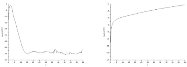
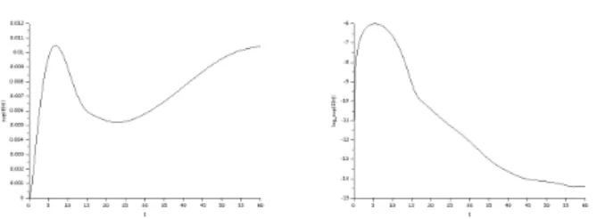
6. Numerical results
In this Section we perform several numerical simulations. Our purpose is two-fold: on the one hand, we check the abil-ity of the scheme in reproducing the expected behavior of the system as asserted in Theorems1and5, in particular con-cerning the energy exchanges, and in capturing the rate of convergence; on the other hand, we also discuss the physical effects and the role of the assumptions in Theorems1and5. We consider the following situations: