Can we trust in numerical computations of chaotic solutions of dynamical systems ?

HAL Id: hal-00682818

https://hal.archives-ouvertes.fr/hal-00682818

Submitted on 27 Mar 2012

HAL is a multi-disciplinary open access

archive for the deposit and dissemination of

sci-entific research documents, whether they are

pub-lished or not. The documents may come from

teaching and research institutions in France or

abroad, or from public or private research centers.

L’archive ouverte pluridisciplinaire HAL, est

destinée au dépôt et à la diffusion de documents

scientifiques de niveau recherche, publiés ou non,

émanant des établissements d’enseignement et de

recherche français ou étrangers, des laboratoires

publics ou privés.

To cite this version:

René Lozi. Can we trust in numerical computations of chaotic solutions of dynamical systems ?.

World Scientific Series on Nonlinear Science, World Scientific, 2013, Topology and Dynamics of Chaos

In Celebration of Robert Gilmore’s 70th Birthday, 84, pp.63-98. �10.1142/9789814434867_0004�.

�hal-00682818�

CAN WE TRUST IN NUMERICAL COMPUTATIONS OF CHAOTIC SOLUTIONS OF DYNAMICAL SYSTEMS ?

R. LOZI

Laboratoire J.A. Dieudonné - UMR CNRS 7351 Université de Nice Sophia-Antipolis

Parc Valrose 06108 NICE Cedex 02

FRANCE E-mail: rlozi@unice.fr

Since the famous paper of E. Lorenz in 1963 numerical computations using computers play a central role in order to display and analyze solutions of nonlinear dynamical systems. By these means new structures have been emphasized like hyperbolic and/or strange attractors. However theoretical proofs of their existence are very di¢ cult and limited to very special linear cases. Computer aided proofs are also complex and require special interval arithmetic analysis. Nevertheless, numerous researchers in several …elds linked to chaotic dynamical systems are con…dent in the numerical solutions they found using popular software and publish without checking carefully the reliability of their results. In the simple case of discrete dynamical systems (e.g. Hénon map) there are concerns about the nature of what a computer …nd out : long unstable pseudo-orbits or strange attractors? The shadowing property and its generalizations which ensure that pseudo-orbits of a homeomorphism can be traceable by actual orbits even if rounding errors are not inevitable are not of great help in order to validate the numerical results. Continuous dynamical systems (e.g. Chua, Lorenz, Rössler) are even more di¢ cult to handle in this scope and researchers have to be very cautious to back up theory with numerical computations. We present a survey of the topic based on these, only few, but well studied models.

To appear in: “From Laser Dynamics to Topology of Chaos,” (celebrating the 70th birthday of Prof Robert Gilmore, Rouen, June 28-30, 2011), Ed. Ch. Letellier.

1. Introduction

Since the famous paper of E. Lorenz in 19631_{, numerical computations using}

com-puters play a central role in order to display and analyze solutions of nonlinear dynamical systems. By these means new structures have been emphasized like hy-perbolic and/or strange attractors. However theoretical proofs of their existence are very di¢ cult and limited to very special linear cases.2 Computer aided proofs are also complex and require special interval arithmetic analysis.3;4 _{Nevertheless,}

numerous researchers in several …elds linked to chaotic dynamical systems are con-…dent in the numerical solutions they found using popular software and publish

without checking carefully the reliability of their results. In the simple case of dis-crete dynamical systems (e.g. Hénon map5_{) there are concerns about the nature}

of what a computer …nd out : long unstable pseudo-orbits or strange attractors?6 The shadowing property which ensures that pseudo-orbits of a homeomorphism can be traceable by actual orbits, even if rounding errors are not inevitable, is not a great help in order to validate the numerical results.7 _Continuous

dynami-cal systems (e.g. Chua, Lorenz, Rössler) are even more di¢ cult to handle in this scope and researchers have to be very cautious to back up theory with numerical computations.8;9 _{We present a survey of the topic based on these, only few, but}

well studied models.10

In Sec. 2 we de…ne the paradigm for possibly ‡awed computations: continu-ous and discrete chaotic dissipative dynamical systems. In Sec. 3, some undesir-able collapsing e¤ects are highligted for an example of strange attractor and for 1-dimensional discrete dynamical systems (logistic and tent maps). The shadow-ing properties (parameter-shifted, orbit-shifted shadowshadow-ing) are presented in Sec. 4, together with the classical mappings of the plane into itself: the Hénon and Lozi maps. Finally in Sec. 5 the case of the seminal Lorenz model and its following metaphors: Rössler and Chua equations is examined.

2. Continuous and discrete chaotic dissipative dynamical systems: a paradigm for possibly ‡awed computations

2.1. Some classes of dynamical system

Dynamical systems are involved in the modeling of phenomena which evolve in time. Their theory attempts to understand, or at least describe in form of mathematical equations, the changes over time that occur in biological, chimical, economical, …nancial, electronical, physical or arti…cial systems. Examples of such systems include the long-term behavior of solar system (sun and planets) or galaxies, the weather, the growth of crystals, the struggle for life between competiting species, the stock market, the formation of tra¢ c jams, etc.

Dynamical systems can be continuous vs discrete, autonomous vs non-autonomous, conservative vs dissipative, linear vs nonlinear, etc. When di¤erential equations are used, the theory of dynamical systems is called continuous dynamical systems. Instead when di¤erence equations are employed the theory is called dis-crete dynamical systems. Some situations may also be modeled by mixed operators such as di¤erential-di¤erence equations. It is the theory of hybrid systems.

In mathematics, an autonomous system or autonomous di¤erential equation is a system of ordinary di¤erential equations which does not explicitly depend on the independent variable, if it is not the case the system is called non-autonomous.

Classical mechanics deals with dynamical systems without damping or friction as the ideal pendula, the solar system. In this case the dynamical systems involved are conservative dynamical systems. When damping or friction occur the dynamical systems are dissipative.

Linear dynamical systems can be solved in terms of simple functions and the behavior of all orbits classi…ed, on the contrary there are in general no explicit solutions of non linear dynamical systems which model more complex phenomena. Before the advent of fast computing machines, solving a non linear dynamical system required sophisticated mathematical techniques and could be accomplished only for a small class of dynamical systems. Numerical methods implemented on computers have simpli…ed the task of determining the orbits of a dynamical system. However when chaotic dynamical systems are studied the crucial question is: can we rely on these solutions ?

Chaos theory studies the behavior of dynamical systems that are highly sensi-tive to initial conditions, an e¤ect which is popularly referred to as the butter‡y e¤ect. Small di¤erences in initial conditions (such as those due to rounding errors in numerical computation) yield widely diverging outcomes for chaotic systems, ren-dering long-term prediction impossible in general. This happens even though these systems are deterministic, meaning that their future behavior is fully determined by their initial conditions, with no random elements involved. In other words, the deterministic nature of these systems does not make them predictable. The …rst example of such chaotic continuous system in the dissipative case was pointed out by the meteorologist E. Lorenz in 1963.1

In this article we limit our study to chaotic (hence non linear) dissipative dy-namical systems, either continuous or discrete, autonomous or non-autonomous. The case of linear system is not relevant because most of the solutions are given by closed formulas. The case of conservative system is much more di¢ cult to han-dle as the lack of friction (dissipation of energy) leads to exponential increasing of rounding errors. Dedicated techniques are necessary to obtain reliable solution.11

Although there exist peculiar mathematical tools in order to study non-autonomous dynamical systems, they can be easily transformed in non-autonomous systems increasing by one the dimension of the space variable. Then we only con-sider autonomous sytems. We focus our study to the most popular models: for the discrete case: logistic and tent map in 1-dimension, Hénon and Lozi map in 2-dimension; for the continuous case: Lorenz, Rössler and Chua model.

2.2. Poincaré map: a bridge between continuous and discrete dynamical system

Generally (i.e. when there exist a periodic solution) the Poincaré map allows us to build a correspondence between continuous and discrete dynamical systems. If we consider a 3-dimensional continuous dynamical system (i.e. a system of three di¤erential autonomous equations):

8 < : : x1= f1(x1; x2; x3) : x2= f2(x1; x2; x3) : x3= f3(x1; x2; x3) (1)

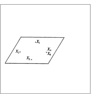
Figure 1. Solutions of a di¤erential system in R3_.

the solution of such a system can be seen as a parametric curve (x1(t) ; x2(t) ; x3(t))

in the space R3_{. A periodic solution (also called a cycle) is no more than a loop in}

this space as shown on Fig. 1 for the solution starting from, and arriving to, the same initial condition X0.

Poincaré map de…ned in a neighborhood of this cycle is the map ' of the plane = R2 into itself which associates to the initial point belonging to this plane, the …rst return point of the solution starting from this very initial point ' : X 2 ! ' (X) 2 (e.g. on Fig. 1. the …rst intersection point X2 of the plane with the

solution starting from X1, ' : X1 2 ! ' (X1) = X2 2 ). Then the study of

n-dimensional continuous system is equivalent to the study of (n 1)-dimensional discrete system.

Figs. 2 and 3 display the discrete periodic orbit fX0; X1; X2; X3; X4= X0g

associated to the continuous periodic orbit of period 4: '(4)(X0) = ' ' ' ' (X0) = X0

3. Collapsing e¤ects

3.1. Undesirable chaotic transient

In 2008, Z. Elhadj and J. C. Sprott12_{introduced a two-dimensional discrete mapping}

with C1 _{multifold chaotic attractors. They studied a modifed Hénon map given}

Figure 2. Discrete periodic orbit associated to the continuous periodic orbit of period 4.

Figure 3. Continuous period 4 orbit.

f (xn; yn) = xn+1 yn+1 = 1 a sin (xn) + byn xn (2)

where the quadratic term x2 _{in the Hénon map (see Sec. 4) is replaced by the}

nonlinear term sin x. They studied this model for all values of a and b. The essential motivation for this work was to develop a C1 _{mapping that is capable}

of generating chaotic attractors with “multifolds”via a period-doubling bifurcation route to chaos which has not been studied before in the literature.

They prove the following theorem on the exitence of bounded orbits

Theorem 3.1. (Elhadj & Sprott) The orbits of the map (2) are bounded for all a 2 R, and jbj < 1, and all initial conditions (x0; x1) 2 R2.

The existence of chaotic attractors is only inferred numerically. They display four examples, convincing at …rst glance, of what they call “chaotic multifold attrac-tors”. Unfortunately one of it obtained for a = 4:0 and b = 0:9 (Fig. 4) is no more than a long transient regime which collapses to a trivial and degenerate behavior: a periodic orbit of period 6 when the computation is done for su¢ cently large value of n. When programming in Language C (BorlandR _{compiler), using a computer}

with Intel DuoCore2 processor and computing with double precision numbers, from any initial points after a transient regime for approximatively 110; 000 iterates (ac-tually the length of the transient regime depends upon the initial value) the orbit is trapped to the period-6 attractor given by:

x120003= 8:95855079898761453 = x120009= x120015= , x120004= 10:96940289429559630 = x120010= x120016= , x120005= 13:06132591362670500 = x120011= , x120006= 8:97249334266406962 = , x120007= 11:90071070225514802 = , x120008= 13:07497800339342220 = .

This attractor is showed on Fig. 5.

Remark 3.1. It is obvious that the phase space (xn; xn+1) on which the points

(xn; xn+1) 2 R2 are computed is …nite when …nite arithmetic replaces continum

state spaces and one can object that every orbit of a mapping must be periodic in this …nite space. However with double precision numbers for each component, it is generally possible (in presence of chaotic attractor) to obtain periodic orbit with period as long as 1011 (see Lozi map in Sec. 4.2) which could be a good approximation for the attractor. Instead an attracting period-6 orbit has a very di¤erent behavior than a strange attractor because such orbit does not possesses the sensitivity to initial condition property, which a minimal necessary condition (but not a su¢ cient one) of existence of chaos.

This example of long chaotic transient regime hiding a periodic attractor with a very short period is not unique in scienti…c literature, numerous researchers in

Figure 4. Chaotic multifold attractor of the map (2) for a = 4:0 and b = 0:9. (Elhadj & Sprott12_).

Figure 5. Period 6 attracting orbit of the map (2) for a = 4:0 and b = 0:9 (Elhadj & Sprott12_).

several …elds linked to chaotic dynamical systems are con…dent in the numerical solutions they found using popular softwares and publish without checking carefully the reliability of their results. Most of the time they compute only few iterates (i.e. few means less than 109_{) of mapping and falsely conclude the existence of chaotic}

regimes upon these numerical clues.

3.2. Enigmatic computations for the logistic map (1838)

In 1838 the belgium mathematician Pierre François Verhulst13 _{introduced a}

di¤er-ential equation modelling the grow of population in a simple demographic model, as an improvement of the Malthusian growth model, in which some resistence to the natural increase of population is added.

dp

dt = mp np 2

p (0) = p0

(3) the function p(t) being the size of the population of the mankind. He latter, in 184514_{, called logistic function the solution of this equation. Putting}

x (t) = n

mp (t) (4)

Eq. 3 is equivalent to

dx

dt = mx (1 x) (5) In 1973, the biologist Sir R. M. May introduced the nonlinear, discrete time dynamical system

xn+1= rxn(1 xn) (6)

as a model for the ‡uctuations in the population of fruit ‡ies in a closed container with constant food.15 _{Due to the similarity of both equations although one is a}

continuous dynamical system, and the other a discrete one, he called Eq. 6 logistic equation. The logistic map fr: [0; 1] ! [0; 1]

fr(x) = rx (1 x) (7)

associated to Eq. 6 and generally considered for r 2 [0; 4] is often cited as an archetypal example of how complex, chaotic behaviour can arise from very simple non-linear dynamical equations.

This dynamical system which has excellent ergodic properties on the real interval [0; 1] has been extensively studied especially by R. M. May16_{, and J. Feigenbaum}17

who introduced what is now called the Feigenbaum’s constant

= 4:669201609102990671853203820466201617258185577::: explaining by a new theory (period doubling bifurcation) the onset of chaos.

For every value of r there exist two …xed points: x = 0 which is always unstable and x = r_r1 _{which is stable for r 2 ]1; 3[ and unstable for r 2 ]0; 1[ [ ]1; 4[ (see Fig.} 6).

When r = 4 , the system is chaotic. The set ( 5 p5 8 ; 5 +p5 8 ) = f0:3454915028; 0:9045084972g

is the period-2 orbit. In fact there exist in…nity of periodic orbits and in…nity of periods (furthermore several distinct periodic orbits having the same period can coexist). This dynamical system possesses an invariant measure

(x) = _p 1 x (1 x) (see Fig. 7).

It is quite surprising that a simple quadratic equation can exhibit such complex behaviour. If the logistic equation with r = 4 modelled the growth of fruit ‡ies, then their population would exhibit erratic ‡uctuations from one generation to another.

In the coordinate sytem

X = 2x 1

Y = 2y 1 (8)

the map of Eq. 7 written in the equivalent form (for r = 4)

g (X) = 1 2X2 (9) was studied in the interval [ 1; 1] by T. S. Ulam and J. von Neumann well before the modern chaos era. They proposed it as a computer random number generator.18 In order to compute periodic orbits whose period is longer than 2 the use of computer is required, as it is equivalent to …nd roots of polynomial equation of degree greater than 4, for which Galois theory teaches that no closed formula is available. However, numerical computation on computer uses ordinarily double precision numbers (IEEE-754) so that the working interval contains roughly 1016 representable points. Doing such a computation19 _{in Eq. 6 with r = 4 with 1,000}

randomly chosen initial guesses, 596, i.e., the majority, converge to the unstable …xed point x = 0, and 404 converge to a cycle of period 15,784,521 (see Table 1a). In an experimental work,20_{O. E. Lanford III, does the same search of numerical}

periodic solution of the logistic equation under the form of Eq. 9. The precise discretization studied is obtained exploiting evenness of this equation to fold the interval [ 1; 0] to [0; 1], i.e. replacing Eq. 9 by

G (X) = 1 2X2 (10) on [0; 1]. It is not di¢ cult to see that the folded mapping has the same set of periods as the original one. In order to avoid the particular discretization of this interval when the standard IEEE-754 is used for double precision numbers, the

Table 1a. Coexisting periodic orbits with 1,000 initial guesses Period Orbit Relative Basin Size

1 _{f0g (unstable …xed point)} 596 over 1; 000 15; 784; 521 Scattered over the interval 404 over 1; 000

Table 1b. Coexisting periodic orbits with 1,000 initial guesses Period Orbit Relative Basin Size

1 _{f0g (unstable …xed point)} 890 over 1; 000 1; 107; 319 Scattered over the interval 2 over 1; 000 3; 490; 273 Scattered over the interval 108 over 1; 000

working interval is then shifted from [0; 1] to [1; 2] by translation, and the iteration of the translated folded map is programmed in straightforward way. Out of 1,000 randomly chosen initial points, 890, i.e., the overwhelming majority, converged to the …xed point corresponding to the unstable …xed point x = 1 in the original representation of Eq. 9, 108 converged to a cycle of period 3,490,273, the remaining 2 converged to a cycle of period 1,107,319 (see Table 1b).

Thus, in both cases at least, the very long-term behaviour of numerical orbits is, for a substantial fraction of initial points, in ‡agrant disagreement with the true behaviour of typical orbits of the original smooth logistic map.

In others numerical experiments we have performed,21;22_{the computer working}

with …xed …nite precision is able to represent …nitely many points in the interval in question. It is probably good, for purposes of orientation, to think of the case where the representable points are uniformly spaced in the interval. The true logistic map is then approximated by a discretized map, sending the …nite set of representable points in the interval to itself.

Describing the discretized mapping exactly is usually complicated, but it is roughly the mapping obtained by applying the exact smooth mapping to each of the discrete representable points and “rounding”the result to the nearest representable point. In our experiments, uniformly spaced points in the interval with several order of discretization (ranging from 9 to 2,001 points) are involved. In each experiment the questions addressed are:

how many periodic cycles are there, and what are their periods ?

how large are their respective basins of attraction, i.e., for each periodic cycle, how many initial points give orbits with eventually land on the cycle in question ?

Table 2 shows coexisting periodic orbits for the discretization with regular meshes of N = 9, 10 and 11 points. There are respectively 3, 2 and 2 cycles. Table 3 displays cases N = 99, 100 and 101 points, there are exactly 2, 4 and 3 cycles. Table 4 stands for regular meshes of N = 1999, N = 2000 and N = 2001

Figure 6. Cobweb diagram of the logistic map f4(x).

points.

It seems that the computation of numerical approximations of the periodic orbits leads to unpredictable and somewhat enigmatic results. As says O. E. Lanford III,20

“The reason is that because of the expansivity of the mapping the growth of roundo¤ error normally means that the computed orbit will remain near the true orbit with the chosen initial condition only for a relatively small number of steps typically of the order of the number of bits of precision with which the calculation is done It is true that the above mapping like many ‘chaotic’mappings satis…es a shadowing theorem (see Sec. 4.3 in this article) which ensures that the computed orbit stays near to some true orbit over arbitrarily large numbers of steps. The ‡aw in this idea as an explanation of the behavior of computed orbits is that the shadowing theorem says that the computed orbit approximates some true orbit but not necessarily that it approximates a typical one.”

He adds, “This suggests the discouraging possibility that this problem may be as hard of that of non equilibrium statistical mechanics”

The existence of very short periodic orbit (Tables 1a, 1b), the existence of a non constant invariant measure (Fig. 7) an the easily recognized shape of the function in the phase space avoid the use of the logistic map as a Pseudo Random Number Generator. However, its very simple implementation in computer program led some authors to use it as a base of cryptosytem.23;24

Figure 7. Invariant measure (x) = p 1

x(1 x) of the logistic map f4(x).

Table 2. Computation on regular meshes of N points N Period Orbit Basin Size

9 1 _f0g 3 over 9 9 1 _f6g 2 over 9 9 1 _{f3; 7g} 4 over 9 10 1 _f0g 2 over 10 10 2 _{f3; 8g} 8 over 11 11 1 _f0g 3 over 11 11 4 _{f3; 8; 6; 9g} 8 over 11

3.3. Collapsing orbit of the symmetric tent map

Another often studied discrete dynamical system is de…ned by the symmetric tent map on the interval J = [ 1; 1]

xn+1= Ta(xn) (11)

Ta(x) = 1 a jxj (12)

Despite its simple shape (see Fig. 8), it has several interesting properties. First, when the parameter value a = 2, the system possesses chaotic orbits. Because of its piecewise-linear structure, it is easy to …nd those orbits explicitly. More, owing to its simple de…nition, the symmetric tent map’s shape under iteration is very well

Table 3. Computation on regular meshes of 99, 100 and 101 points N Period Orbit Basin Size

99 1 _f0g 3 over 99 99 10 _{f3; 11; 39; 93; 18; 58; 94; 15; 50; 97g} 96 over 99 100 1 _f0g 2 over 100 100 1 _f74g 2 over 100 100 6 _{f11; 39; 94; 18; 58; 96g} 72 over 100 100 7 _{f7; 26; 76; 70; 82; 56; 97g} 24 over 100 101 1 _f0g 3 over 101 101 1 _f75g 2 over 101 101 1 _{f19; 61; 95g} 96 over 101

Table 4. Computation on regular meshes of 1; 999, 2; 000 and 2; 001 points N Period Orbit Basin Size

1999 1 _f0g 3 over 1999 1999 4 _{f554; 1601; 1272; 1848g} 990 over 1999 1999 8 _{f3; 11; 43; 168; 615; 1702; 1008; 1997g} 1006 over 1999 2000 1 _f0g 2 over 2000 2000 1 _f1499g 14 over 2000 2000 2 _{f691; 1808g} 138 over 2000 2000 3 _{f376; 1221; 1900g} 6 over 2000 2000 8 _{f3; 11; 43; 168; 615; 1703; 1008; 1998g} 1840 over 2000 2001 1 _f0g 5 over 2001 2001 1 _f1500g 34 over 2001 2001 2 _{f691; 1809g} 92 over 2001 2001 8 _{f3; 11; 43; 168; 615; 1703; 1011; 1999g} 608 over 2001 2001 18 _{f35; 137; 510; 1519; 1461; 1574; g} 263 over 2001 2001 25 _{f27; 106; 401; 1282; 1840; 588; g} 1262 over 2001

understood. The invariant measure is the Lebesgue measure. Finally, and perhaps the most important, the tent map is conjugate to the logistic map, which in turn is conjugate to the Hénon map (see Sec. 4.1) for small values of b.25

However the symmetric tent map is dramatically numerically instable: Sharkovski¼¬’s theorem applies for it.26 _{When a = 2 there exists a period three}

orbit, which implies that there is in…nity of periodic orbits. Nevertheless the orbit of almost every point of the interval J of the discretized tent map eventually wind up to the (unstable) …xed point x = 1 (this is due to the binary structure of ‡oating points) and there is no numerical attracting periodic orbit.27

The numerical behaviour of iterates with respect to chaos is worse than the numerical behaviour of iterates of the approximated logistic map. This is why the tent map is never used to generate numerically chaotic numbers.

Figure 8. Tent map T2(x).

3.4. statistical properties

Many others examples could be given, but those given may serve to illustrate the intriguing character of the results, the outcomes proves to be extremely sensitive to the details of the experiment, but the …ndings all have a similar ‡avour: a relatively small number of cycles attract near all orbits, and the lengths of these signi…cant cycles are much larger than one but much smaller than the number of representable points. P. Diamond and al.28;29, suggest that statistical properties of the phenomenon of computational collapse of discretized chaotic mapping can be modelled by random mappings with an absorbing centre. The model gives results which are very much in line with computational experiments and there appears to be a type of universality summarised by an Arcsin law. The e¤ects are discussed with special reference to the family of dynamical systems

xn+1= 1 j1 2xnjl; 06 x 6 1; 1 6 l 6 2 (13)

Computer experiments show close agreement with prediction of the model. How-ever these results are of statistical nature, they do not give accurate information on the exact nature of the periodic orbits (e.g. length of the shortest or the great-est one, size of their basin of attraction ...). Following this work, G. Yuan and J. A. Yorke30 study precisely the collapse to the repelling …xed point x = 1 of the iterates of the one dimensional dynamical system

xn+1= 1 2 jxnjl; 16 x 6 1; l > 2 (14)

equally spaced from 1 to +1 (as we have done in Sec. 3.2). The map associated to this system

Ta;l(x) = 1 a jxjl

being an usual nonlinear generalization of the map Ta(x) of Eq. 12. They not only

prove rigorously that the collapsing e¤ect does not vanish when arbitrarily high numerical precision is employed, but also they give a lower bound of the probability for which it happens. They de…ne Pcollapsewhich is the probability that there exists

n such that xn = 1 and they give the proof that Pcollapse depends only on the

numbers N and l. The lower bound of Pcollapseis given by

lim inf N!1Pcollapse> p K0[1 erf (K0)] exp (K0)2> 0 (15) K0= lK 12 1=:2 1=l 1 + (2l)1=l 1 2 1=2 K = 1 X i=1 k2_i !1=2 ki= l h (i + 1=2)1=l (i 1=2)1=li with erf(x) = p2 Z x 0 e t2dt (16) They plot the curve given by Eq. 15 along with the numerical results (Figure 9). Each numerical datum is obtained as follows. For each l they sample 10; 000 pairs of l; x from(l 0:01l; l + 0:01l) ( 1; 1)with uniform distribution. For each sample they keep iterating the dynamical system de…ned by Eq. 14 with the initial condition x until the numerical trajectory repeats. Then they calculate the portion of trajectories that eventually map to 1. The deviation is clear since Eq. 15 only gives a lower bound. Nonetheless the theoretical curve reveals the fact that Pcollapse

is already substantial for l = 3 and it predicts that Pcollapseincreases as l increases

and that liml!1Pcollapse= 1.

4. Shadowing and parameter-shifted shadowing property of mappings of the plane

4.1. Hénon map (1976) found by mistake

The chaotic behavior of mapping of the real line is relatively simple compared to the behavior of mapping on the plane. These mappings could be seen as a simple expansion in a phase space with increased dimension of both models (logistic and tent) we have introduced in the previous section. However they have been discovered not in this “ascending” way, instead they come in “descending way” as metaphor of Poincaré map of 3-D continuous dynamical systems.

Figure 9. Pcollapseas a function of l. The curve in this …gure is the lower bound computed from

Eq. 15. Numerical results are obtained by using di¤erent numerical precisions are also shown in this …gure "+" -double precision " " -single precision " "-…xed precision 10 12_(from30_).

Figure 10. Observatory of Nice, the o¢ ce of Michel Hénon was located inside the building.

In order to study numerically the properties of the Lorenz attractor1_{, M. Hénon}

an astronom of the observatory of Nice, France (see Fig. 10) introduced in 19765_a

simpli…ed model of the Poincaré map of this attractor. The Lorenz attractor being in dimension 3, the corresponding Poincaré map is a map from the plane R2_{to R}2_.

The Hénon map is then also de…ned in dimension 2 as

Ha;b:

x y =

y + 1 ax2

It is associated to the dynamical system

xn+1= yn+ 1 ax2n

yn+1= bxn

(18)

For the parameter value a = 1:4, b = 0:3, M. Hénon pointed out numerically that there exists an attractor with fractal structure. This was the …rst example of strange attractor (previously introduced by D. Ruelle and F. Takens31_{) for a}

mapping de…ned by an analytic formula.

As highlighted in the sequence of Figs. 11-14, the like-Cantor set structure in one direction orthogonal to the invariant manifold in this simple mapping was a dramatic surprise in the community of physicists and mathematicians.

Nowadays hundreds of research papers have been published on this prototyp-ical map in order to fully understand its innermost structure. However as for 1-dimensional dynamical systems, there is a discrepancy between the mathematical properties of this map in the plane and the numerical computations done using (IEEE-754) double precision numbers.

If we call Megaperiodic orbits,6_{those whose length of the period belongs to the}

interval of natural numbers 106_{; 10}9 _{and Gigaperiodic orbits, those whose length}

of the period belongs to the interval 106_{; 10}9 _{, Hénon map possesses both Mega}

and Gigaperiodic orbits. On a Dell computer with a Pentium IV microprocessor running at 1.5 Gigahertz frequency, using a Borland C compiler and computing with ordinary (IEEE-754) double precision numbers, one can …nd for a = 1:4 and b = 0:3 one attracting period of length 3; 800; 716; 788, i.e. two hundred forty times longer than the longest period of the one-dimensional logistic map (Table 1a). This periodic orbit (we call it here Orbit 1) is numerically slowly attracting. Starting with the initial value

(x0; y0)1= ( 0:35766; 0:14722356)

one winds up:

(x11;574;730;767;y11;574;730;767)1= (x15;375;447;555;y15;375;447;555)1

= (1:27297361350955662; 0:0115735710153616837) The length of this period is obtained subtracting

15; 375; 447; 555 11; 574; 730; 767 = 3; 800; 716; 788

However this Gigaperiodic orbit is not unique: starting with the other initial value (x0; y0)2= (0:4725166; 0:25112222222356)

(x12;935;492;515;y12;935;492;515)2= (x13;246;439;123;y13;246;439;123)2

= (1:27297361350865113; 0:0115734779561870744) Remark 4.1. This second orbit can be reached more rapidly starting form the other initial value

(x0; y0) = (0:881877775591; 0:0000322222356)

then

(x4;459;790;707; y4;459;790;707) = (1:27297361350865113; 0:0115734779561870744)

Remark 4.2. It is possible that some others periodic orbits coexist with both Orbit 1 and Orbit 2. However there is no peculiar method but the brute force to …nd it if any.

Remark 4.3. The comparison between Orbit 1 and Orbit 2 gives a perfect idea of the sensitive dependence on initial conditions of chaotic attractors:

Orbit 1 passes through the point

(1:27297361350955662; 0:0115735710153616837) and Orbit 2 passes through the point

(1:27297361350865113; 0:0115734779561870744)

The same digits of the coordinates of these points are bold printed, they are very close.

The discovery of a strange attractor for maps of the plane boosted drastically the research on chaos in the years 70’. This is miraculous considering that if M. Hénon tried to test rigorously his model nowadays with powerful computers he should only found long periodic orbits. In 1976, M. Hénon used the electronic pocket calculator built by Hewlett-Packard company HP-65 (Fig. 15) and one of the only two computers available at the university of Nice a IBM 7040 (Fig.16), the other one was a IBM 1130, slower. The HP-65 …rst introduced in 1974 was worth 750 e (equivalent to 3; 500 e nowadays), the IBM 7040, was worth 1,100,000 e (equivalent to 7; 800; 000 e in the year 2012).

He concluded,5 _{“The simple mapping (4) (i.e. Eq. 17 in this article) appears}

to have the same basic properties as the Lorenz system. Its numerical exploration is much simpler: in fact most of the exploratory work for the present paper was carried out with a programmable pocket computer (HP-65). For the more exten-sive computations of Figures 2 to 6, we used a IBM 7040 computer, with 16-digit accuracy. The solutions can be followed over a much longer time than in the case of a system of di¤erential equations. The accuracy is also increased since there are no integration errors. Lorenz (1963) inferred the Cantor-set structure of the attractor

Figure 11. Hénon strange attractor, 10000 successive points obtained by iteration of the mapping.

from reasoning, but could not observe it directly because the contracting ratio after one ‘circuit’was too small: 7 10 5_{. A similar experience was reported by Pomeau}

(1976). In the present mapping, the contracting ratio after one iteration is 0:3, and one can easily observe a number of successive levels in the hierarchy. This is also facilitated by the larger number of points. Finally, for mathematical studies the mapping (4) might also be easier to handle than a system of di¤erential equations.”

The large number of points was in fact very few5_{: “The transversal structure}

(across the curves) appears to be entirely di¤erent, and much more complex. Al-ready on Figures 2 and 3 (i.e. Fig. 11 in this article) a number of curves can be seen, and the visible thickness of some of them suggests that they have in fact an underlying structure. Figure 4 (i.e. Fig. 12 in this article) is a magni…ed view of the small square of Figure 3: some of the previous ‘curves’are indeed resolved now into two or more components. The number n of iterations has been increased to 105_{, in order to have a su¢ cient number of points in the small region examined.}

The small square in Figure 4 is again magni…ed to produce Figure 5 (i.e. Fig. 13 in this article), with n increased to 106_{: again the number of visible ‘curves’}

in-creases. One more enlargement results in Fig. 6 (i.e. Fig. 14 in this article), with n = 5 106_{: the points become sparse but new curves can still easily be traced.”}

In 1976, the one million e, IBM 7040 took several hours to compute …ve millions points, today a basic three hundred euros laptop, runs the same computation in one hundredth of a second.

With so few iterations nowadays the following claim5_{: “These …gures strongly}

Figure 12. Enlargement of the squared region of Figure 11. The number of computed points is increased to n = 105_.

that each apparent ‘curves’ is in fact made of an in…nity of quasi-parallel curves. Moreover, Figures 4 to 6 indicate the existence of a hierarchical sequence of ‘levels’, the structure being practically identical at each level save for a scale factor. This is exactly the structure of a Cantor set.” should be obviously untrue. One can assert that Hénon map was found not by chance (the reasoning of M. Hénon was straightforward) but by mistake. It is a great luck for the expand of chaos studies!

4.2. Lozi map (1977) a tractable model

Using one of the …rst desktop electronic calculator HP-9820, he usually employed for initiate to computer sciences, mathematics teacher trainees, R. Lozi found out, on june 15, 1977, (on the scienti…c campus of the university of Nice, few kilome-ters apart of the observatory of this town of the French Riviera where M. Hénon worked), that the linearized version of the Hénon map displayed numerically the same structure of strange attractors, but the curves were replaced by straight lines. He published this result in the proceedings of a conference on dynamical systems which held in Nice in july of the same year,32 _{in a very short paper of one and an}

half pages.

The aim of R. Lozi, a numerical analyst, was to allow algebraic computations on an analog of the Hénon map, such direct computation being untractable on the original model due to the square function. He changed this function with a absolute value, de…ning the map

Figure 13. Enlargement of the squared region of Figure 12, n = 106_.

Figure 14. Enlargement of the squared region of Figure 13, n = 5 106_.

La;b :

x y =

y + 1 _{a jxj}

Figure 15. Electronic pocket calculator HP-65.

Figure 16. Computer IBM 7040.

and the associate dynamical system

xn+1= yn+ 1 a jxnj

yn+1= bxn

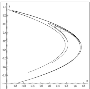
Figure 17. Lozi map L1:7;0:5.

He then found out on the plotter device attached to his small primitive computer that for the value a = 1:7, b = 0:5, the same Cantor-set like structure was apparent. Due to the linearity of this new model, it is possible to compute explicitly any periodic orbit solving a linear system. Moreover in december 1979, M . Misiurewicz2

gave a talk in the famous conference organized in december 1979 at New-York by the New-York academy of science in which he etablished rigorously the proof that what he call “Lozi map” has a strange attractor for some parameter values (including the genuine one a = 1:7, b = 0:5). Since that time, hundreds of papers have been published on the topic.

Remark 4.4. _{The open set M of the parameter space (a; b) where the existence} of strange attractor is proved is now called the Misiurewicz domain. It is de…ned as

0 < b < 1; a > b + 1; 2a + b < 4; ap2 > b + 2; b < a

2 ₁

(2a + 1) (21) Today, in the same conditions of computation as for Hénon map (see Sec. 4.1), running the computation during nineteen hours, one can …nd a Gigaperiodic at-tracting orbit of period 436; 170; 188; 959 more than one hundred times longer than the period of Orbit 1 found for the Hénon map.

Starting with

(x0; y0) = (0:88187777591; 0:0000322222356)

(x686;295;403;186;y686;295;403;186) = (x250;125;214;227;y250;125;214;227)

= (1:34348444450739479; 2:07670041497986548:10 7) There is a transient regime before the orbit is reached. It seems that there is no periodic orbit with a smaller length. This could be due to the quasihyperbolic nature of the attractor. However, the parameter-shifted shadowing property, the orbit-shifted shadowing property of Lozi map (and generalized Lozi map), which are new variations of the shadowing the property which ensures that pseudo-orbits of a homeomorphism can be traceable by actual orbits even if rounding errors in computing are not inevitable, has been recently proved.7;33

4.3. Shadowing, parameter-shifted shadowing and orbit-shifted shadowing properties

The shadowing property is the property which ensures that pseudo-orbits (i.e. or-bits computed numerically using …nite precision number) of a homeomorphism can be traceable by actual orbit. The concept and primary results of shadowing prop-erty for uniformly hyperbolic di¤eomorphisms were introduced by D. V. Anosov34

and R. Bowen,35 _{who proved that such di¤eomorphisms have the shadowing}

prop-erty. Various papers associated with shadowing property and uniform hyperbolicity were presented by many authors. Comprehensive expositions on these works were included in books by K. Palmer36_{or S. Y. Pilyugin.}37

The precise de…nition of this property is38

De…nition 4.1. _{(Shadowing) Let (X; d) a metric space, f : X ! X a function and} let _{> 0. A sequence fx}kgqk=p, (p; q) 2 N2of points is called a -pseudo-orbit of f if

d (f (xk) ; xk+1) < for p k q 1 (e.g. a numerically computed orbit is a

pseudo-orbit). Given _{> 0, the pseudo-orbit fx}kgq_k=p, is said shadowed by x 2 X, if

d fk_{(x) ; x}

k < for p k q. One says that f has the shadowing property if

for > 0 there is > 0 such that every -pseudo-orbit of f can be shadowed by some point.

However, if one relaxes the uniform hyperbolicity condition on di¤eomorphisms slightly (Lozi map, for example, has not such a property), then many problems con-cerning the shadowing property are not solved yet. Nowadays, it is widely supposed that many di¤eomorphisms producing chaos would not have the shadowing property. In fact, Yuan and Yorke39 _{found an open set of absolutely}

nonshad-owable C1 _{maps for which nontrivial attractors supported by partial hyperbolicity}

include at least two hyperbolic periodic orbits whose unstable manifolds have di¤er-ent dimensions. Moreover, Abdenur and Díaz40_{showed recently that the shadowing}

property does not hold for di¤eomorphisms in an open and dense subset of the set of C1_{-robustly nonhyperbolic transitive di¤eomorphisms.}

In order to …x this issue the notion of the parameter-shifted shadowing property (for short PSSP ) was introduced by E. M. Coven, I. Kan and J. A. Yorke.41 _In

fact, they proved that the tent map (Eq. 12) has the parameter-…xed shadowing property for almost every sloop a in the open interval I = (p2; 2); but do not have it for any a in a certain dense subset of I. Moreover, they proved that, for any a 2 I, the tent map Ta has PSSP. The de…nition of this variant property being33

De…nition 4.2. _{(PSSP) Let ff}ag_a2J be a set of maps on R2 where J is an open

interval in R.

For _{> 0, the sequence fx}ngn>0 R2 is called -pseudo-orbit of fa if

kfa(xn) xn+1k for any integer n> 0.

For a 2 J, we say that fahas the parameter shif ted shadowing property

if, for any > 0, there exist = (a; ) > 0; ~a = ~_{a (a; ) 2 J such that any} -pseudo-orbit fxngn=0 of fa can be -shadowed by an actual orbit of fa~,

that is, there exists a y 2 R2_{such that kf}n ~

a (y) xn+1k for any n> 0.

For Lozi map, S. Kiriki and T. Soma proof that33

Theorem 4.1. _{There exists a nonempty open set O of the Misiurewicz domain M} such that, for any (a; b) 2 O, the Lozi map La;b has the parameter-shifted shadowing

property in a one-parameter family fLa;b~ g~a2J …xing b, where J is a small open

interval containing a.

However they note that “The problem of parameter-…xed shadowability is still open even for the Lozi family as well as the Hénon family.”

Another variation of shadowability is the orbit-shifted shadowing property (for short OSSP ) recently introduced by A. Sakurai7_{in order to study generalized Lozi}

maps introduced by L.-S. Young.42The limited extend of this article does not allow us to recall the complex de…nition of these generalized maps.

De…nition 4.3. For 0> 0, 1> 0, and > 0, with 0 0, a sequence fxngn=0

in R = [0; 1] [0; 1] is an ( 0; 1) shif ted pseudo orbit of f if, for any n 1,

xn and xn+1satisfy the following conditions.

(i) _{kf (x}n) xn+1k if B 0(xn 1) \ (S1[ S2) = ;.

(ii) kf (xn) ( 1; 0) xn+1k if B 0(xn 1) \ S16= ;.

(iii) kf (xn) + ( 1; 0) xn+1k if B 0(xn 1) \ S26= ;.

where S1and S2 are the two components of the essential singularity set of f .

De…nition 4.4. (OSSP) We say that f has the orbit-shifted shadowing property if, for any > 0 with ₀, there exist 0; 1; > 0 such that any ( 0; 1)

shif ted pseudo _{orbit fx}ngn=0in R of f can be -shadowed by an actual orbit

of f , that is, there exists z 2 R such that kfn_{(z) x}

nk for any n 0.

Theorem 4.2. Any generalized Lozi map f satisfying the conditions (2.1)–(2.4) given in7 _{has the orbit-shifted shadowing property. More precisely, for any 0 <}

0, there exists > 0 such that any ( ; =2)-shifted -pseudo-orbit of f in R is

-shadowed by an actual orbit.

For sake of simplicity, we do not give the technical conditions (2.1)-(2.4), however one can proof that any original Lozi maps La;b indicated in Theorem 4.1 satis…es

these conditions.

In conclusion to both Secs. 3 and 4, it appears that if, owing to the introduction of computers since forty years, it is easy to compute orbits of mapping in 1 or 2-dimension (and more generally in …nite dimension), it is not unproblematic to obtain reliable results. The mathematical study of what is actually computed (for the orbits) is a rather di¢ cult and still challenging problem. Trusty results are obtained under rather technical assumptions. Considering a new mathematical tool, the Global Orbit Pattern (GOP ) of a mapping on …nite set, R. Lozi and C. Fiol19;21 _{obtain some combinatorial results in 1-dimension.}

There is not place in this paper to consider other computations than the compu-tations of orbits. However there is a need for several others reliable numerical results as the Lyapunov numbers,43 the fractal dimensions (correlation, capacity, Hauss-dor¤,...) and Lyapunov spectrum ,44_{topological entropy,}45_{extreme value laws.}46;47

...The researches are very active in these …elds. One can mention as an example the relationship between the expected value of the period scales and the correlation dimension for the case of fractal chaotic attractors of D-dimensional maps.48

Theorem 4.3. The expected value of the period scales with round o¤ is

m = D=2 (22)

where D is the correlation dimension of the chaotic attractor. The periods m have substantial statistical ‡uctuation. That is, P (m), the probability that the period is m, is not strongly peaked around m. This probability is given by

P (m) = 1 m F p 8m m ! (23) where F (x) = r 8 1 r 2 erf x p 2 (24)

and erf(x) is de…ned by Eq.16

5. Continuous models

We have highlighted the close relationship between continuous and discrete models via Poincaré map. We have also pointed out that M. Hénon constructed his model in order to compute more easily Poincaré map of the Lorenz model which is crunching too fast for direct numerical computations. It is time to study directly these initial equations together with the metaphorics ones which that follows naturally: the Rössler and the Chua equations.

5.1. Lorenz attractor (1963)

The following non linear system of di¤erential equations was introduced by E. Lorenza _{in 1963.}1 _{As a crude model of atmospheric dynamics, these equations led}

Lorenz to the discovery of sensitive dependence of initial conditions - an essential factor of unpredictability in many systems (e. g. meteorology).

8 < : : x = (x + y) : y = x y xz : z = xy z (25)

Numerical simulations for an open neighbourhood of the classical parameter values

= 10; = 28; = 8

3 (26)

suggest that almost all points in phase space tend to a strange attractor the Lorenz attractor. One can note that the system is invariant under the transformation

S(x; y; z) = ( x; y; z) (27) This means that any trajectory that is not itself invariant under S must have a symmetric “twin trajectory.” For > 1 there are three …xed points: the origin and the two “twin points”

C = p ( 1); p ( 1); 1

For the parameter values generally considered, C have a pair of complex eigen-values with positive real part, and one real, negative eigenvalue. The origin is a saddle point with two negative and one positive eigenvalue satisfying

0 < 3< 3< 1< 2

Thus the stable manifold of the origin Ws_{(0) is two dimensional and the unstable}

manifold of the origin Wu_{(0) is one dimensional. As indicated by M. Hénon}5_{in his}

initial publication the ‡ow contracts volumes at a signi…cant rate (see Sec. 4.1). As the divergence of the vector …eld is ( + + 1) the volume of a solid at time t can be expressed as

V (t) = V (0)e ( + +1)t V (0)e 13:7t

a_{Edward Lorenz, born on May, 23, 1917 at west Hartford (Connecticut), dead on April, 16, 2008}

at Cambridge (Massachusset), studied the Rayleigh-Bénard problem (i. e. the motion of a ‡ow heated from below, as an approach of the atmospheric turbulence) using a primitive Royal McBee LPG-30 computer. He …rst considered series of 12 di¤erential equations when he discovered the "butter‡y e¤ect". Then he simplied his model from 12 to only three equations. As for Hénon model, his discovery was made by mistake due to rounding errors.

Figure 18. Lorenz attractor.

for the classical parameter values. This means that the ‡ow contracts volumes almost by a factor one million per time unit which is quite extreme. There appears to exist a forward invariant open set U containing the origin but bounded away from C . The set U is a double torus (one with two holes), with its holes centered around the two excluded …xed points. If one lets ' denote the ‡ow of Eq. 25, there exists the maximal invariant set

A = \

t=0

' (U; t)

Due to the strong dissipativity of the ‡ow, the attracting set A must have zero volume. As indicated by W. Tucker49_{, it must also contain the unstable manifold}

Wu_{(0) of the origin, which seems to spiral around C in a very complicated non}

periodic fashion (see Fig. 18).

In particular A contains the origin itself, and therefore the ‡ow on A can not have a hyperbolic structure. The reason is that …xed points of the vector …eld generate discontinuities for the return maps (Poincaré maps), and as a consequence, the hyperbolic splitting is not continuous. Apart from this, the attracting set appears to have a strong hyperbolic structure.

5.2. Geometric Lorenz attractor

As it was very di¢ cult to extract rigorous information about the attracting set A from the di¤erential equations themselves, M. Hénon constructed his famous model (Sec. 4.1) in order to understand numerically its inner structure. In another way of

research, a geometric model of the Lorenz ‡ow was introduced by J. Guckenheimer and R. Williams50 _{at the end of the seventies (see Fig. 19). This model has been}

extensively studied and it is well understood today. The question whether or not the original Lorenz system for such parameter values has the same structure as the geometric Lorenz model has been unsolved for more than 30 years. By combina-tion of normal form theory and rigorous computacombina-tions, W. Tucker51 _{answered this}

question a¢ rmatively, that is, for classical parameters, the original Lorenz system has a robust strange attractor which is given by the same rules as for the geometric Lorenz model. From these facts, it is known that the geometric Lorenz model is crucial in the study of Lorenz dynamical systems. Oddly enough the original equa-tions introduced by Lorenz have remained a puzzle until the same author proved in 1999 in his Ph.D Thesis49 _{the following theorem}

Theorem 5.1. For the classical parameter values, the Lorenz equations support a robust strange attractor A. Furthermore the ‡ow admits a unique SRB measure X

with supp ( _{X) = A.}

Remark 5.1. SRB measures, are an invariant measures introduced by Ya. Sinai, D. Ruelle and R. Bowen in the 1970’s. These objects play an important role in the ergodic theory of dissipative dynamical systems with chaotic behavior. Roughly speaking, SRB measures are the invariant measures most compatible with volume when volume is not preserved. They provide a mechanism for explaining how local instability on attractors can produce coherent statistics for orbits starting from large sets in the basin.

In addition, W. Tucker indicates, “In fact, we prove that the attracting set is a singular hyperbolic attractor. Almost all nearby points separate exponentially fast until they end up on opposite sides of the attractor. This means that a tiny blob of initial values soon smears out over the entire attractor. It is perhaps worth pointing out that the Lorenz attractor does not act quite as the geometric model predicts. The latter can be reduced to an interval map which is everywhere expanding. This is not the case for the Lorenz attractor: there are large regions in the attracting set that are contracted in all directions under the return map. However, such regions only require a few more iterations before accumulating expansion. This corresponds to the interval map being eventually expanding, and does not lead to any di¤erent qualitative long time behaviour. Apart from this, the Lorenz attractor is just as the geometric model predicts: it contains the origin, and thus has a very complicated Cantor book structure.”

One of the many ingredients required for the proof of this theorem is a rigourous arithmetics on a trapping region consisting in 350 adjacent rectangles belonging to the return plate z = 27 = 1. W. Tucker says “One major advantage of our numerical method is that we totally eliminate the problem of having to control the global e¤ects of rounding errors due to the computer’s internal ‡oating point representation. This is achieved by using a high dimensional analogue of interval

Figure 19. Geometric Lorenz model from52

arithmetic. Each object (e. g. a rectangle or a tangent vector) subjected to computation is equipped with a maximal absolute error , and can thus be represented as a box = [ 1 1; 1+ 1] [ n n; n+ n].

When following an object from one intermediate plane to another, we compute upper bounds on the images of i+ i, and lower bounds on the images of i i,

i = 1; ; n. This results in a new box e _e, which strictly contains the exact image of . To ensure that we have strict inclusion, we use quite rough estimates on the upper and lower bounds. This gives us a margin which is much larger than any error caused by rounding possibly could be. Hence, the rounding errors are taken into account in the computed box e _e, and we may continue to the following intermediate plane by restarting the whole process.

As long as we do not ‡ow close to a …xed point, the local return maps are well de…ned di¤eomorphisms, and the computer can handle all calculations. Some rectangles, however, will approach the origin (which is …xed point), and then the computations must be interrupted as discussed in the previous section (i. e. the normal form theory).”

The work of W. Tucker is a big step forward reliability of numerical solution of chaotic continuous dynamical system. However it has been obtained after a great deal of e¤ort (he published two revised versions of the proof anytime he detected a mistake in the code) which can not be a¤orded to any new continuous chaotic model.

Figure 20. Lorenz map from.52

5.3. Lorenz map

In contrast the analysis of the Poincaré map associated to the geometric model of the Lorenz ‡ow allows the use of the parameter-shifted shadowing property.52 This …rst return map on a Poincaré cross section of a geometric Lorenz ‡ow is called a Lorenz map L : _{n !} , where = _{(x; y) 2 R}2_{; jxj ; jyj 6 1 and}

= (0; y) 2 R2_{; jyj 6 1 . More precisely it is de…ned as follows}

De…nition 5.1. (Lorenz map) Let denote the components of _{n with 3} ( 1; 0) (see Fig. 19). A map L : _{n ! , is said to be a Lorenz map if it is a} piecewise C1 di¤eomorphism which has the form

L (x; y) = ( (x) ; (x; y))

where _{: [ 1; 1] n f0g ! [ 1; 1] is a piecewise C}1_{-map with symmetric property}

( x) = (x) and satisfying

limx!0+ (x) = 1; (1) < 1

limx!0+ 0(x) = 1; 0(x) >p2 for any x 2 (0; 1]

(see Fig. 20a), and : _{n ! [ 1; 1] is a contraction in the y-direction. Moreover,} it is required that the images L ( +), L ( ) are mutually disjoint cusps in , where

the vertices v+, v of L ( +) are contained in f 1g [ 1; 1] respectively (see Fig.

20b).

Then, S. Kiriki and T. Soma proved the parameter-shifted shadowing property (PSSP ) for Lorenz maps.52

Theorem 5.2. _{There exists a de…nite set L of Lorenz maps satisfying the following} condition:

For any L 2 L and any > 0, there exist > 0 and > 0 such that any pseudo orbit of the Lorenz map L with L (x; y) = L (x; y) ( x; 0) is shadowed by an actual orbit of L.

Theorem 5.3. _{Any geometric Lorenz ‡ow controlled by a Lorenz map L 2 L has} the parameter-shifted shadowing property.

Due to the lack of space, we refer to52 _{for the strict description of L.}

Besides this work on the Lorenz map, there are many some others rigorous results on Lorenz equations. Z. Galias and P. Zygliczy´nski,53;54 _{for example, are}

basing their result on the notion of the topological shifts maps (TS-maps). Let = (x; y; z) 2 R3_{; z = 1 which is the standard choice for the Poincaré section.}

Let P be a Poincaré map generated on the plane by Eq. 25, they prove that: Theorem 5.4. For all parameter values in a su¢ cently small neighborhood of pa-rameter value given by Eq. 26, there exists a transversal section I such that the Poincaré map P induced by Eq. 25 is well de…ned and continuous on I. There exists a continuous surjective map : Inv I; P2 _!

2, such that

P2=

The preimage of any periodic sequence from 2 contains periodic points of P2.

Remark 5.2. The maximal invariant part of I (with respect to P2_{) is de…ned by}

Inv I; P2 =\

i2Z

P_jI2i(I)

and 2 = f0; 1; ; K 1gZ is a topological space with the Tichonov topology;

0; 1; ; K 1 being symbols characterizing periodic in…nite sequences of TS-maps (see4 _{fore more details).}

In this case the Poincaré map is issued directly from Lorenz equations not from the geometric model. Due to the limited extend of this article, we do not cite all the results on computer aided proof. We refer the reader to.4

5.4. Rössler attractor (1976)

We have seen that from the seminal discovery of the Lorenz attractor, several strate-gies have been developped in order to study this appealing and complex mathemat-ical object: geometric Lorenz model, Lorenz map, Hénon map (and Lozi map as linearized version). In 1976 O. E. Rössler followed a di¤erent direction of research: instead of simplify the mathematic equation 25 and considering that, due to extreme simplifaction, there is no actual link between this equation and the Rayleigh-Benard problem from which it is originate, he turned his mind to the study of a chemical

Figure 21. Rössler attractor.

multi-vibrator. He started to design some three-variable oscillator based on a two-variable bistable system coupled to a slowly moving third-two-variable. The resulting three-dimensional system was only producing limit cycles at the time. At an inter-national congress on rhythmic functions held on September 8-12, 1975 in Vienna, he met A. Winfree, a theoretical biologist who challenged him to …nd a biochemi-cal reaction reproducing the Lorenz attractor. Rössler failed to …nd a chemibiochemi-cal or biochemical reaction producing the Lorenz attractor but, he instead found a sim-pler type of chaos in a paper he wrote during the 1975 Christmas holidays.55 _The

obtained chaotic attractor (see Fig. 21) 8 < : : x = y z : y = x + ay : z = b + z(x c) (28) a = 0:2; b = 0:2; c = 5:7 (29) does not have the rotation symmetry of the Lorenz attractor (de…ned by Eq. 27), but it is characterized by a map equivalent to the Lorenz map.

The reaction scheme (see Fig. 22) leading to Eq. 28 is meticulously analyzed by Ch. Letellier and V. Messager.56

The structure of the Rössler attractor is simpler than the Lorenz’s one. However even if hundreds of papers has been written on it, the rigorous proof of its existence is not yet established as done for Lorenz equations. In 1997, P. Zygliczy´nski using reducted Rössler equations to two parameters instead of three (i. e. stating that

Figure 22. Combination of an Edelstein switch with a Turing oscillator in a reaction system producing chaos. E = switching subsystem, T = oscillating subsystem; constant pools (sources and sinks) have been omitted from the scheme as usual (From,56_{adapted from.}55₎

a = b in Eq. 28) gave, using computer assisted proof similar results as he did for Lorenz equations.4

Let =n_{(x; y; z) 2 R}3_{; x = 0; y < 0; x > 0}o

Theorem 5.5. For all parameter values in a su¢ cently small neighborhood of (a; c) = (0:2; 5:7) there exists a transversal section N such that the Poincaré map P induced by Eq. 28 is well de…ned and continuous. There exists a continuous surjective map _{: Inv (N; P) !} 3, such that

P= A (Inv (N; P)), where A = 2 4 0 1 1 0 1 1 1 0 0 3 5

The preimage of any periodic sequence from A contains periodic points of P.

As this result is related to the Poincaré map of Rössler equations, nowadays there is still a need to apply the method developed by W. Tucker to prove the true existence of a strange attractor.

5.5. Chua attractor (1983)

Before he discovered his equations, O. Rössler in collaboration with F. Seelig, in-spired by a little book entitled Measuring signal generators, Frequency Measuring Devices and Multivibrators from the Radio-Amateur Library,57_{began to “translate”}

electronic systems into nonlinear chemical reaction systems. The know-how he de-veloped led eventually in to his chaotic model. Few years later, in october 1983, visiting T. Matsumoto at Waseda University, L. O. Chua found an electronic circuit (see Fig. 23) mimicking directly on an oscilloscope screen a chaotic signal (see Fig. 24). As we have seen, only two autonomous systems of ordinary di¤erential equa-tions were generally accepted then as being chaotic, the Lorenz equaequa-tions and the Rössler equations. The nonlinearity in both systems is a function of two variables namely, the product function which is very di¢ cult to build in electronic circuit. L. O. Chua58 _{says, “I was to have witnessed a live demonstration of presumably}

the world’s …rst successful electronic circuit realization of the Lorenz Equations, on which Professor Matsumoto’s research group had toiled for over a year. It was in-deed a remarkable piece of electronic circuitry. It was painstakingly breadboarded to near perfection, exposing neatly more than a dozen IC components, and embellished by almost as many potentiometers and trimmers for …ne tuning and tweaking their incredibly sensitive circuit board. There would have been no need for inventing a more robust chaotic circuit had Matsumoto’s Lorenz Circuit worked. It did not. The fault lies on the dearth of a critical nonlinear IC component with a near-ideal characteristic and a su¢ ciently large dynamic range; namely, the analog multiplier. Unfortunately, this component was the key to building an autonomous chaotic cir-cuit in 1983.” He adds, “Prior to 1983, the conspicuous absence of a reproducible functioning chaotic circuit or system seems to suggest that chaos is a pathological phenomenon that can exist only in mathematical abstractions, and in computer simulations of contrived equations. Consequently, electrical engineers in general, and nonlinear circuit theorists in particular, have heretofore paid little attention to a phenomenon which many had regarded as an esoteric curiosity. Such was the state of mind among the nonlinear circuit theory community, circa 1983. Matsumoto’s Lorenz Circuit was to have turned the tide of indi¤erence among nonlinear circuit theorists. Viewed from this historical perspective and motivation, the utter dis-appointments that descended upon all of us on that uneventful October afternoon was quite understandable. So profound was this failure that the wretched feel-ing persisted in my subconscious mind till about bedtime that evenfeel-ing. Suddenly it dawned upon me that since the main mechanism which gives rise to chaos, in both the Lorenz and the Rössler Equations, is the presence of at least two unstable equilibrium points - 3 for the Lorenz Equations and 2 for the Rössler Equations - it seems only prudent to design a simpler and more robust circuit having these attributes.

Having identi…ed this alternative approach and strategy, it becomes a simple exercise in elementary nonlinear circuit theory to enumerate systematically all such

Figure 23. Chua’s circuit from.61

circuit candidates, of which there were only 8 of them, and then to systematically eliminate those that, for one reason or another, can not be chaotic.”

The Chua’s equations

8 < : : x = (y (x)) : y = x y + z : z = y (30) (x) = x + g (x) = m1x + 1 2(m0 m1) [jx + 1j jx 1j] (31) = 15:60; = 28:58; m0= 1 7; m1= 2 7 (32)

where soon carefully analyzed by T. Matsumoto.59 _{The main mathematical idea}

Figure 24. Chua attractor.

Hénon map by linearizing the parabola with an absolute value as done in Lozi map six years before (even if L. O. Chua did not know these maps at that time).

The “nonlinear” characteristic which is in fact only piecewise linear allows some exact computations. Henceforth, L. O. Chua et al. proved very soon that the mechanism of chaos exists in this attractor.60 _{However in spite it is}

pos-sible to obtain closed formula for the solution of Eqs. 30 in every subspace fx 1g ; f 1 < x < 1g ; f1 xg ; due to the transcendental nature of the equa-tion allowing the computaequa-tion at the matching boundaries fx = 1g ; fx = 1g, of the global solution,9_{it is not possible to compute it explicitely. As only numerically}

computed solutions are avaliable, it remains the gnawing problem of what is really computed. To that problem may be added the fact that the electronic realization of the Chua’s circuit is not exactly governed by Eqs. 30, due to the instability of the electronics components, the parameter value (Eq. 32) is randomly ‡uctuating around its mean value. It is very di¢ cult to analize the experimental observed chaos.61

One possible way to perform this analysis may be the use of a new mathematical tool: con…nor instead of attractor.62 The con…nor theory, when applied to Chua’s circuit allowed the discovery of coexisting chaotic regimes.8;63

6. conclusion

We have shown, in the limited extend of this article, on few but well known examples,10_{that it is very di¢ cult to trust in numerical solution of chaotic}

obtain reliable results. We have focused our survey on models related to the seminal Lorenz model which is the most studied model of strange attractor. These models are not the only one studied today. Countless models presenting chaos, arising in every …elds concerned with dynamics such as ecology, biology, chimistry, economy, …nance, electronics ..., are developped since forty years. However their study is less carefully done as those presented here, conducting sometimes to hasty results and ‡awed theories in these sciences. In addition the disturbing phenomenom of “ghost solution”can appears when discretization of nonlinear di¤erential equation by cen-tral di¤erence scheme is used (several examples of such ghost solutions when cencen-tral di¤erence scheme is used sole or in combination with Euler’scheme, are given by M. Yamaguti and al.64_{). Recently A. N. Sharkovsky and S. A. Berezovsky}65 _pointed

out the notion of “numerical turbulence” which appears, due to incorrectness of calculation method stipulated by discreteness. In conclusion one can say that there is room for more study of the relationship between numerical computation and theoretical behavior of chaotic solutions of dynamical systems.

References

1. E. N. Lorenz, “Deterministic nonperiodic ‡ow,” J. Atmospheric Science, 20, 130-141 (1963).

2. M. Misiurewicz, “Strange attractors for the Lozi mappings,” Ann. New-York Acad. Sci., 357 (1), 348-358 (1980).

3. W. Tucker, “The Lorenz attractor exists,” C. R. Acad. Sci. Paris Sér. I Math., 328 (12), 1197-1202 (1999).

4. P. Zygliczy´nski, “Computer assisted proof of chaos in the Rössler equations and the Hénon map,” Nonlinearity, 10 (1), 243-252 (1997).

5. M. Hénon, “A Two-dimensional mapping with a strange attractor,” Commun. Math. Phys., 50, 69-77 (1976).

6. R. Lozi, “Giga-periodic orbits for weakly coupled tent and logistic discretized maps,” Modern Mathematical Models, Methods and Algorithms for Real World Systems, eds. A. H. Siddiqi, I. S. Du¤ & O. Christensen, (Anamaya Publishers, New Delhi, India), 80-124 (2006).

7. A. Sakurai, “Orbit shifted shadowing property of generalized Lozi maps,” Taiwanese J. Math., 14 (4), 1609-1621 (2010).

8. R. Lozi & S. Ushiki, “Coexisting chaotic attractors in Chua’s circuit,” Int. J. Bifur-cation & Chaos, 1 (4), 923-926 (1991).

9. R. Lozi & S. Ushiki, “The theory of con…nors in Chua’s circuit: accurate analysis of bifurcations and attractors,” Int. J. Bifurcation & Chaos, 3 (2), 333-361 (1993). 10. D. Blackmore, “New models for chaotic dynamics,” Regular & Chaotic dynamics, 10

(3), 307-321 (2005).

11. J. Laskar & P. Robutel, “The chaotic obliquity of the planets,” Nature, 361, 608-612 (1993).

12. Z. Elhadj & J. C. Sprott, “A two-dimensional discrete mapping with C1 multifold chaotic attractors,” Elec. J. Theoretical Phys., 5 (17), 1-14 (2008).

13. P.-F. Verhulst, “Notice sur la loi que la population poursuit dans son accroissement,” Correspondance mathématique et physique de l’observatoire de Bruxelles, 4 (10), 113-121 (1838).