Publisher’s version / Version de l'éditeur:
Proceedings of the ASME 2011 International Mechanical Engineering Congress &
Exposition (IMECE2011), 2011-11-17
READ THESE TERMS AND CONDITIONS CAREFULLY BEFORE USING THIS WEBSITE. https://nrc-publications.canada.ca/eng/copyright
Vous avez des questions? Nous pouvons vous aider. Pour communiquer directement avec un auteur, consultez la
première page de la revue dans laquelle son article a été publié afin de trouver ses coordonnées. Si vous n’arrivez pas à les repérer, communiquez avec nous à [email protected].
Questions? Contact the NRC Publications Archive team at
[email protected]. If you wish to email the authors directly, please see the first page of the publication for their contact information.
NRC Publications Archive
Archives des publications du CNRC
This publication could be one of several versions: author’s original, accepted manuscript or the publisher’s version. / La version de cette publication peut être l’une des suivantes : la version prépublication de l’auteur, la version acceptée du manuscrit ou la version de l’éditeur.
Access and use of this website and the material on it are subject to the Terms and Conditions set forth at
Optimum angles for multi-angle elastic light scattering experiments
Burr, D. W.; Daun, K. J.; Thomson, K. A.; Smallwood, G. J.
https://publications-cnrc.canada.ca/fra/droits
L’accès à ce site Web et l’utilisation de son contenu sont assujettis aux conditions présentées dans le site LISEZ CES CONDITIONS ATTENTIVEMENT AVANT D’UTILISER CE SITE WEB.
NRC Publications Record / Notice d'Archives des publications de CNRC:
https://nrc-publications.canada.ca/eng/view/object/?id=0a8d6fff-682c-4a42-9b10-c645c12fc13a https://publications-cnrc.canada.ca/fra/voir/objet/?id=0a8d6fff-682c-4a42-9b10-c645c12fc13a
Proceedings of the ASME 2011 International Mechanical Engineering Congress & Exposition IMECE2011 November 11-17, 2011, Denver, Colorado, USA
IMECE2011-64748DRAFT
OPTIMUM ANGLES FOR MULTI-ANGLE ELASTIC LIGHT SCATTERING
EXPERIMENTS
D. W. Burr and K. J. Daun
Department of Mechanical and Mechatronics Engineering, University of Waterloo Waterloo, ON, Canada
K. A. Thomson and G. J. Smallwood
Institute for Chemical Process and Environmental Technology, National Research Council Canada Ottawa, ON, Canada
ABSTRACT
In multiangle elastic light scattering (MAELS) experiments, the morphology of aerosolized particles is inferred by shining collimated radiation through the aerosol and then measuring the scattered light intensity over a set of angles. In the case of soot-laden aerosols MAELS can be used to recover, among other things, the size distribution of soot aggregates. This involves solving an ill-posed set of equations, however. While previous work focused on regularizing this inverse problem using Bayesian priors, this paper presents a design-of-experiment methodology for identifying the set of measurement angles that minimizes its ill-posedness. The inverse problem produced by the optimal angle set requires less regularization and is less sensitive to noise, compared with two other measurement angle sets commonly used to carry out MAELS experiments.
INTRODUCTION
In most combustion processes pyrolized fuel molecules coalesce into nanospheres between 10 and 100 nm in diameter, called primary particles, which in turn agglomerate to form soot aggregates. Soot has long been a focus of combustion research, in large part because its formation within gas turbines and automotive engines is closely linked to the performance of these devices. Accordingly, designing the next generation of clean and efficient combustion technology relies on improved understanding of soot formation and soot models, which in turn is predicated on the availability of soot measurements carried out within engines and flames.
Soot also strongly impacts both human health and the environment through mechanisms that depend strongly on aggregate size. Epidemiologists have recently discovered that small soot particles penetrate more deeply into the lungs and can even cross the pleural membrane into the bloodstream [1]. Climatologists and atmospheric scientists have also assessed soot to be an extremely potent factor in climate change, second
only to carbon dioxide [2]: soot deposited on glaciers increase their absorption of sunlight and hasten glacial melting [3], for example; while soot in the atmosphere acts as condensation nuclei for clouds that shield the earth from solar irradiation, which may drastically alter local climatic patterns [4]. Accordingly, instrumentation for measuring both the size and quantity of soot produced by a combustion device is crucial for assessing its impact on human health and the environment, and its compliance to emissions regulations. Often the size distribution of soot aggregates within an aerosol is quantified in terms of the number of primary particles per aggregate, Np.
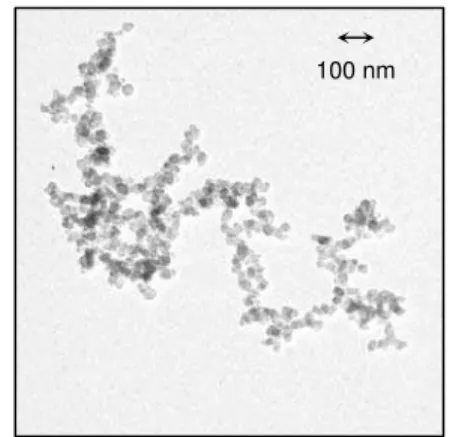
While it is possible to infer the size distribution of aggregates within a soot-laden aerosol through transmission electron microscopy of extracted soot aggregates, such as the image shown in Fig. 1, this process has a number of drawbacks. Perhaps foremost, charactering the soot aggregate size distributions requires the capture and processing of thousands of electron micrographs, an extremely time-intensive endeavor, which effectively disallows analysis of transient data. Also, inferring three-dimensional structural information from 2-D
Fig. 1: Transmission electron micrograph of soot aggregates.
projections of the soot aggregates may induce certain biases in the results [5]. Finally, obtaining the physical access needed to probe an aerosol is often difficult (for example in a combustion chamber) and the probe itself may have a perturbing effect on the physical and chemical processes occurring within the aerosol.
Optical diagnostics overcome many drawbacks of physical sampling. One such technique is multi-angle elastic light scattering (MAELS) [6], in which collimated light, usually from a laser, is shone through the aerosol. The aggregate size distribution is then inferred from the angular distribution of scattered light. A schematic of this experiment is shown in Fig.1. The angular distribution of the scattered light intensity,
g, and the aggregate size distribution, PNp, are related by a
Fredholm integral equation of the first kind,
1 , p p p g C K N P N dN
(1)where C is a scaling coefficient that depends on the experimental apparatus, the aggregate number density, Nagg, and
the optical properties of soot, K(,Np) is the kernel function
derived from light scattering theory, and P(Np) is the probability
density for the number of primary particles per aggregate. Equation (1) is derived from the radiative transfer equation using Rayleigh-Debye-Gans Polydisperse Fractal Aggregate (RDG-PFA) theory to provide the required scattering cross-sections of the soot aggregates [6, 7]. Predicting the angular distribution of scattered light, g(), for a specified P(Np) can be
done by carrying out the integration; this is called the forward
problem. Solving the inverse problem, i.e. recovering PNp
from g, on the other hand, is mathematically ill-posed due to the smoothing action of K(,Np). When carrying out the
integral in Eq. (1), moderate changes in P(Np) are smoothed by K(, Np) into comparatively smaller changes in g().
Conversely, then, small perturbations in g(), which are inevitable in an experimental setting, are amplified into large variations in P(Np).
`The aggregate size distribution is usually found by assuming a distribution shape for P(Np),most often lognormal,
and then solving for the distribution parameters that best explain the MAELS data through nonlinear regression [8].
Information about the size distribution, including the ratio of
moments for P(Np) can also be found by plotting the
normalized scattering intensity as a function of the modulus of the scattering wave vector, q() = 2sin(/2)/, where is the wavelength of light, and then identifying features of scattering regimes [6]. These treatments do not directly address the fundamentally ill-posed nature of the inverse problem, however.
In a previous work [7], we demonstrated that P(Np) can be
found by solving a matrix analogue of Eq. , Ax = b, where b contains the angular scattering measurements, x is a discrete form of P(Np) taken to be piecewise uniform over n
evenly-spaced subdomains of width Np, and Aij is derived from K(,Np) The smoothing property of K(,Np makes A
ill-conditioned, which amplifies the noise contaminating the data into a very large error component in the recovered aggregate sizes. In [7] we showed that this issue can be addressed by
regularizing the problem, a process in which extra information about the assumed character of P(Np), for example smoothness
and non-negativity, is added to the problem. While regularization permits deconvolution of the MAELS data, however, it also inherently biases the recovered solution towards the analyst’s expectations, since these expectations are used to supplement the information content of Ax=b, which is inadequate by itself to specify a unique or stable solution for x.
When the MAELS problem is written in matrix form it is clear that ill-posedness of the underlying experiment, and consequently the ill-conditioning of A, depends on the angles at which scattered light is measured. Researchers often use uniform angular increments between the minimum and maximum measurement angles. Sorensen [6] suggested, instead, that angles be chosen to produce uniform increments in the scattering wave vector modulus, q41sin(/2), where
is the laser wavelength. This paper presents a rigorous methodology based on design-of-experiment theory that will produce a set of measurement angles that minimizes the ill-conditioning of the deconvolution problem.
NOMENCLATURE
A Coefficient matrix
b Vector of scattering intensities
C Scaling coefficient
dp Primary particle diameter
f(,Rg) Scattering form factor g() Scattered light intensity at
i0 Incident laser intensity
K(,Np) Light scattering kernel
Np Number of primary particles in an aggregate
P(Np) Probability density of Np
q Modulus of the scattering wave vector
RgNp) Radius of gyration wi ith singular value
x Discrete vector representation of P(Np)
Tikhonov regularization parameter
b Error in measured data
Fig. 2: Schematic of a MAELS experiment.
Detector + optics Laser + optics g() i0
x Error in recovered distribution 2 Chi-squared function
Solid angle
Wavelength of laser light
() Scattering phase function
Matrix of singular values
s, Scattering coefficient
Scattering measurement angle
Set of scattering measurement angles
DERIVATION OF THE GOVERNING EQUATIONS
The scattered light incident on the detector, g(), is obtained by solving the radiative transfer equation [9] for the geometry shown in Fig. 2. This analysis is simplified through a number of assumptions: absorption and emission of light by the medium are small relative to the intensity of the scattered light;
i0 is vertically polarized and undergoes a single scattering
event between the laser and the detector; background intensity is negligible; and finally, the laser beam is assumed to have a top-hat profile, i.e. a constant intensity across the beam width.
Combined, these assumptions reduce the RTE to
exp , ,0 ( ) sin 4 s w g C i (2)where is the solid angle subtended by the laser viewed from the measurement volume, which is defined by the intersection of the laser and the detection optics, Cexp depends on the
collection optics and photoelectric conversion efficiencies, s
and () are the bulk scattering coefficient and scattering phase function of the aerosol. The phase function and scattering coefficient are found by integrating the relevant scattering cross-sections of a soot aggregate of size Np over all
possible size classes, weighted by the probability density of the aggregate size class, P(Np).
The scattering cross-sections for an aggregate containing
Np primary particles are approximated using
Rayleigh-Debye-Gans Polyfractal Aggregate (RDG-PFA) theory [6], which is premised on the assumption the primary particles are much smaller than the wavelength of laser light so that each primary particle “sees” a uniform wave field, and that the primary particles scatter independently. Through these simplifications Eq. (2) can be rewritten in the form of Eq. (1) with the kernel that depends on Np and [7],
,
2
sin p g p p N f q R N K N (3)where RgNp is the radius of gyration of the aggregate, f() is
the form factor, and q() is the modulus of the scattering wave vector. Due to the nature of diffusion-limited agglomeration the soot aggregates have a self-similar, fractal-like structure and consequently Rg is related to Np by a power-law relationship,
1 2 f D p p f g p d N k R N (4)where dp is the primary particle diameter, which usually obeys a
comparatively narrow distribution in an aerosol [10] and can therefore be approximated as constant, and kf2.4 and Df1.72 are typical values of the fractal prefactor and
dimension for soot formed in laminar flames as well as overfire soot formed in turbulent flames.
The form factor has been derived in a number of different ways over the Guinier and power-law scattering regimes. The model chosen for this work is [11]
8 2 8 8 , 1 3 f D g g p g f qR f q R N qR D (5)The remaining terms related to the primary particle size parameter (dp/), aggregate number density, parameters
related to the experimental apparatus, and the bulk optical properties of soot are absorbed into the coefficient, C [7]. SOLUTION BY LINEAR ALGEBRA
The majority of techniques described in the literature for recovering an aggregate size distribution from MAELS data rely on specifying a distribution shape for P(Np) and then
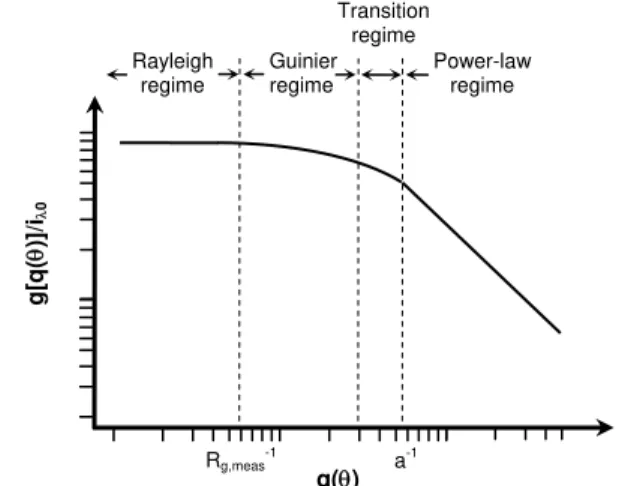
performing nonlinear regression to recover the distribution parameter (e.g. [8]). Information about the aggregate sizes can also be obtained by plotting the normalized scattered intensity
gfi,0 as a function of the modulus of the scattering wave
vector, q(), shown schematically in Fig. 3. This curve reveals that light scattering occurs in three distinct regimes: the Rayleigh regime; the Guinier regime; and the power law regime. An additional transition regime is often identified between the Guinier and power-law regimes. Most information relating to aggregate size is found from the Guinier regime, in which the normalized scattering intensity follows [6]
0 2, 2
1 1 3 g meas i R q g q (6)where Rg,meas is the effective radius of gyration if the soot
aggregates within the aerosol were monodisperse. The distribution width can be inferred by the relation [6]
Fig. 3: Plotting the normalized scattering intensity versus the modulus of the scattering wave vector reveals that angular scattering from soot-laden aerosol occurs in distinct regimes. Guinier regime Rg,meas -1 g[q ( )]/i 0 Power-law regime Rayleigh regime Transition regime q() a -1
2 2 2 2 2 , 2 Df D f g meas f M R a k M (7)
where a=dp/2 is the primary particle radius. By plotting g[q()]/i0 and specifying a distribution shape, then, Eqs. (6)
and (7) can be used to infer the unknown distribution parameters.
It is preferable, however, to recover P(Np) without
imposing a distribution type. In our previous paper [7] we showed that this can be done by specifying a maximum aggregate size, Np,max, beyond which P(Np) is assumed to be
zero. Next, the domain Np is discretized into n sub-domains of
uniform width Np, as shown in Fig. 4, over each of which P(Np) is assumed to be uniform. If scattered light is measured
at a set of m angles, the deconvolution problem reduces to solving Ax = b, where big(i), xjP(Np,j) and A is an (mn)
matrix having elements defined as
, , 2 * * , 2 p j
p p j p N N ij i p p N N A C K N dN (8)Unfortunately, the underlying ill-posedness of the deconvolution problem causes A to be ill-conditioned. In the context of the matrix problem, deconvolution of MAELS data equates to solving
exact exact
Ax A x δx b δb b (9)
where b contains measurement noise. The ill-conditioning of A amplifies b into a very large error term x, relative to x.
The extent of ill-conditioning can be quantified through a singular value decomposition (SVD) on A, A=UVT
, where the column vectors of U and V form an orthonormal basis for b and x, respectively, and the diagonal matrix contains the singular values wj arranged in decreasing order. Since the
inverse of an orthonormal matrix is simply its transpose the solution to Eq. (9) can be written explicitly as
1 1 1
T T exact T n n n j j j j j j j wj j wj j wj u b u b u δb x v v v (10)where vj and uj are column vectors of V and U, respectively.
The rank-nullity theorem guarantees that all singular values are
strictly positive as long as m ≥ n and the scattering
measurements are independent (which is generally satisfied for unique measurement angles) but the smoothing property of
K(Np) causes some of these singular values to be very small.
These small singular values produce an error term (the second term on the RHS of Eq. (10)) that dominates x.
The small singular values are due to the fact that the information content of A is barely sufficient to uniquely specify x from the observed angular scattering data in b, which makes the solution susceptible to measurement noise. (Letting n > m results in a singular matrix, in which case the information content of A is inadequate to specify a unique solution.) It is therefore necessary to use regularization, which adds extra information based on the expected solution attributes, including smoothness, small magnitude, and non-negativity, to reduce this ambiguity and eliminate the small singular values. The drawback of regularization, however, is that it biases the outcome towards the analyst’s expectation, with little indication in the form of an elevated residual due to the ill-conditioning of A. Consequently, it is often difficult to discern how reliant the recovered solution is on a priori assumptions about the solutions’ attributes.
OPTIMAL DESIGN OF EXPERIMENTS
Expressing the MAELS deconvolution problem in the form of Eq. (10) reveals that the extent of ill-conditioning is determined entirely by A, which in turn is a function of the set of measurement angles, . It follows, then, that the choice of plays an important role in experimental accuracy. Nevertheless many researchers simply choose uniform angular spacing between the minimum and maximum angles permitted by the apparatus. Sorensen [6] suggested that a better approach may be to choose angles based on uniform increments in q() rather than , based on the prominence of q() in the underlying light scattering equations.
The fact that it is possible to predict the extent of ill-conditioning based on the singular values suggests that there may be a more rigorous way to choose the measurement angles. The first step is to define an objective function, f(), that is minimized by the set of angles that produces the least ill-conditioned matrix. If the measurements in b are mutually-independent and each obeys an unbiased normal distribution with a standard deviation, i, a chi-squared function can be
defined as
2 2 1
n i i i i b a x x (11)where ai is the ith row of the A matrix. Minimizing 2x is
equivalent to maximizing the likelihood function, while the value of 2
(x*) at its minimum quantifies the agreement between the data in b and the most probable solution x*Exexact in other words, 2(x*) indicates the degree of agreement between modeled and measured data, in the context of the measure data subject to normally distributed error.
If the rows in Ax = b is scaled so that the standard deviations are equal, then Eq. (11) becomes
2 2 1 T x Ax b Ax b (12) Fig 4: Discretization of P(Np). 0 50 100 150 200 P(N p ) Np 0 0.005 0.010 0.015 0.020 Np Np,maxwhich is minimized by x* = A-1b. Substituting x = x*+x into Eq. (12) and simplifying gives
2 2 1 T T δx δx A Aδx (13)which defines a confidence interval traced out by the vector x with its tail on x* for a given value of 2 corresponding to a tabulated probability. For a specified value of 2
, the confidence interval is a hyperellipse in n space [12, 13]. The hyperellipse volume indicates to what extent the measurement noise in b is amplified into a solution error, x, so the objective of this analysis is to design the experiment so that the hyperellipse volume is minimized. Since 2 and 2
are constants, the vector x can only be made small by making ATA as large as possible. There are a number of ways to maximize this value [12]; in this work this is done by minimizing the objective function
det T
f θ A θ A θ (14)
which is equivalent to increasing the singular values of A
through the identity
2 1 det
n T j j w A A (15)(By convention, optimization problems are usually cast as minimization problems, which is why the objective is to minimize det(ATA) rather than maximize det(ATA).) Geometrically, the hyperellipse corresponding to 2
= 1 has principle axes in the directions of the column vectors of V, scaled by the inverse of the corresponding singular value. Hence, making the singular values as large as possible minimizes the volume of the hyperellipse.
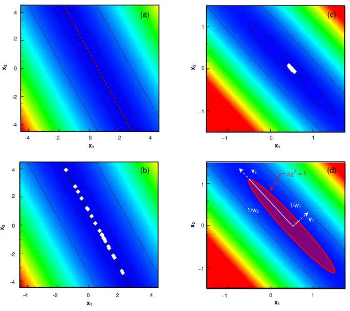
An instructive 2-D example is shown in Fig. 5 corresponding to the linear problem
1 1 1 2 2 2 2 4 2 2 1 1 exact exact x x b b x x Ax b (16)
where b1 and b2 are sampled from an unbiased normal
distribution of width = 0.1, and is a heuristic parameter used to change A. The case of = 0 corresponds to a singular A matrix since the first row is twice the second row, and the
Fig. 5: Example of optimal design of experiments, corresponding to Eq. (14).
4 2 -4 -2 0 -4 -2 0 2 4 x2 x1 4 2 -4 -2 0 -4 -2 0 2 x2 x1 4 x2 x1 1 0 1 1 0 1 x2 x1 1 0 1 1 0 1 (a) (b) (d) (c) v2 v1 2 = 1 1/w1 1/w2
2
contours in Fig. 5 (a) show that the information content of A is inadequate to specify a unique solution for x; instead there exists a locus of solutions along the dotted red line that make 2(x) = 0. Setting 0.002, shown in Fig. 5 (b), admits a
unique solution for x, but the singular values of A are very small and consequently x is very large. Making = 2, as shown in Fig. 5 (c), increases the singular values of A and decreases the ellipse volume. The geometric relationship between the ellipse volume corresponding to 2
= 1, the column vectors of V, and the singular values, are shown in Fig. 5 (d).
OPTIMIZATION OF MAELS MEASUREMENT ANGLES The above methodology is applied to optimize a set of 23 measurement angles for the MAELS experiment described in [7, 8]. Minimization started from an initial solution vector *
filled with uniformly-spaced angles between 23° and 160°, which are the minimum and maximum angles permitted by the apparatus; these values were imposed as bound constraints throughout the minimization procedure.
We initially attempted to minimize f using Newton’s method, but this approach failed due to its multimodal nature; this can be seen inFig. 6 which is a plot of f() with all angles fixed at their nominal values except 20, which is varied
between 23° and 160°. Accordingly, we switched to simulated annealing; in contrast to gradient-based methods, which always choose a descent direction, simulated annealing periodically accepts an uphill direction with a probability that increases with a heuristically-defined annealing temperature, T. This parameter is initially large enough to allow the algorithm to “hop” out of shallow local minima, but is progressively reduced as the solution hones in on a deep local minimum. The performance of the algorithm is verified by using it to minimize
f() with 20 as the only free variable and the rest held at 0.
Figure 6 shows that simulated annealing finds the global minimum of this univariate problem.
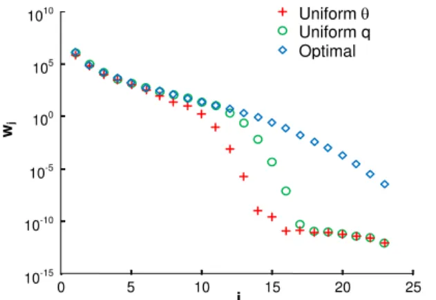
The optimal set of angles found by minimizing f() are shown in Table 1, along with measurement angle sets that are uniformly spaced in the and q domains, the two most
common approaches presently used in MAELS experiments. The singular values of the A matrix formed by each of the angle sets are plotted in Fig. 7, which verifies that the optimal angle sets produce larger singular values compared to the other two sets. The smaller singular values should correspond to a smaller hyperellipse volume and less measurement noise amplification. Equivalently, the distributions corresponding to larger singular values should require less regularization to stabilize the deconvoltuion of the MAELS data, thereby reducing the influence of regularization-induced biased into the recovered aggregate size distribution.
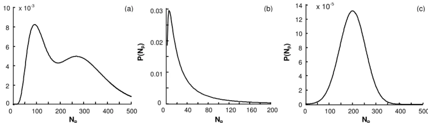
EVALUATION OF MAELS MEASUREMENT ANGLES The performance of these three measurement angle sets are compared by solving synthetic MAELS experiments on three candidate distributions shown in Fig. 8: a bimodal distribution; a lognormal distribution fit to a histogram of P(Np) derived
Fig. 6: Plot of f() allowing 20 to vary with other angles
held at their nominal values.
Table 1: MAELS measurement angles
Uniform increments [degrees] Uniform q increments [degrees] Optimized [degrees] 10 10 10 23.0 14.5 11.8 29.6 19.3 13.7 36.1 24.2 15.3 42.6 29.1 16.7 49.1 34.1 18.1 55.7 39.2 19.5 62.2 44.4 20.8 68.7 49.6 22.2 75.2 54.9 23.7 81.7 60.4 25.4 88.3 66.1 27.1 94.8 71.9 29.1 101.3 78.0 31.4 107.8 84.3 34.0 114.3 90.9 37.1 120.9 98.0 40.9 127.4 105.7 45.8 133.9 114.0 52.2 140.4 123.5 61.3 147.0 134.6 75.6 153.5 149.4 102.0 160 160 160
Fig. 7: Singular values of A matrices generated using the measurement angle sets.
0 5 10 15 20 25 10-15 10-10 10-5 100 105 1010 wj j Uniform Uniform q Optimal 20 [rad] 0.5 1 1.5 2 2.5 10-25 10-20 10-15 10-10 10-5 20(simulated annealing) f
from electron microscopy [10]; and a normal distribution corresponding to larger soot aggregates. In each case, the specified P(Np) is substituted into Eq. (1) and the integral is
evaluated numerically to generate three vectors containing unperturbed data, bexact, corresponding to the three sets of measurement angles shown in Table 1.
Even in the case of the optimized measurement angles, the magnitude of singular values shown in Fig. 7 indicates that, in the presence of measurement noise the A matrix is too ill-conditioned to recover x by direct inversion. To this end we use standard Tikhonov regularization, which augments Ax = b with a second equation, Ix = 0, thereby promoting a solution having a small Euclidean norm. The distribution is then recovered by solving the linear least-squares problem
2 2 arg min 0 A b x x I (17)
where is a regularization parameter, which determines the influence of the prior assumption, in this case a small solution norm, relative to the information contained in the scattering data.
Regularized solutions have two error components: perturbation error caused by amplification of the noise in the data, b; and regularization error due to the fact that the prior information used to stabilize the inversion process is not entirely consistent with the true solution. Increasing the level of regularization reduces perturbation error, but too much regularization causes oversmoothing. A major challenge of inverse analysis is to identify the regularization parameter that minimizes the total error, which is the sum of these two components.
If the exact solution is known, however, the regularization and perturbation errors can be determined through a perturbation analysis of Ax = b [14],
#
exact exact exact
x x x A b δb (18)
which leads to an expression for the total error in x,
#
# exact exact
δx x A b A δb (19)
where xexact is the true solution, x= A#b = A#(bexact+b) is the regularized solution, and A# is the regularized pseudoinverse of A, which can be formed from the SVD of the augmented matrix. The perturbation error is given by pert = A#b, the
regularization error is regxexactA#bexact, and the total
error is given by totx.
We first attempt to recover x using an unperturbed dataset, i.e. b=bexact. As noted above, however, even with b=0 some
regularization must be applied to recover physically-meaningful solutions. The minimum level of regularization needed to recover each imposed distribution is shown in Table 2 for the different sets of measurement angles. In all cases the optimized measurement angles require the least amount of regularization to reconstruct x, since these angles produce the least ill-conditioned A matrices.
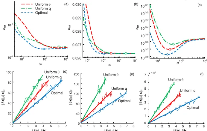
Next, we attempt to recover distributions from datasets contaminated with artificial noise. Each element of b is sampled from a normal distribution with a width of = 0.03. Figure 9 shows the perturbation error, regularization error, and total error found using various levels of Tikhonov regularization to recover the bimodal distribution shown in Fig. 8 (a). As noted above, perturbation error decreases monotonically with increasing , while regularization error follows the opposite trend. The total error, which is the sum of these two components, has a minimum at an intermediate value of . The total errors for the three different distributions are shown in Fig. 10 (a-c); in each case, the optimal angle has the smallest total error, also corresponding to the least amount of regularization.
Alternatively we can compare the performance of the measurement angle sets by choosing a constant and then varying the amount of measurement noise. Further
manipulation of Eq. (19) and employing the identity
ab≤|ab results in
#
δx δb
A A
x b (20)
Table 2: Minimum regularization required to reconstruct x with b = 0.
Bimodal Lognormal Normal
Uniform 9.875 9.875 1.757
Uniform q 2.232 0.233 0.233
Optimal 0.067 0.232 0.004
Fig. 8: Aggregate size distributions used to evaluate the measurement angle sets: (a) bimodal; (b) lognormal; and (2) normal distributions. 0 100 200 300 400 500 x 10-5 (c) 0.01 0.02 0.03 (b) 100 200 300 400 500 0 2 4 6 8 10 x 10-3 ) (a) P(N p ) P(N p ) P(N p ) Np Np Np 0 0 40 80 120 160 200 0 0 2 4 6 8 10 12 14
where A#A is the modified condition number of A. Figure 10 (d-f) shows that the normalized solution error, xx, is indeed linearly proportional with the normalized measurement error, bb for solutions obtained using the values in Table 2, and that in all three cases the reconstructions obtained using the optimized measurement angles are least sensitive to perturbation error.
Some physical insight into why the optimized angles outperform the other two sets is obtained by superimposing the angles over a plot of the normalized angular scattering intensity,
g()/i0, versus q2() shown in Fig. 11. As noted above,
information about PNp. Figure 10 shows that the
measurement angles that are uniformly spaced in the q and domains are clustered towards large values of q2. This part of the curve corresponds to power-law scattering, and should appear as a straight line when plotted on a log-log graph, and therefore can be defined from relatively few measurements; therefore, multiple measurements made in this regime provide nearly superfluous data. On the other hand, the uniformly-spaced angle sets (both and q space) have comparatively few points allocated to define the more complex curvature of the transition regime, suggesting that more information could be extracted about P(Np) by locating measurement angles in this
scattering regime, thereby reducing the underlying ill-posedness of this problem.
The set of optimized angles, in contrast, are more densely concentrated within the Guinier and transition regimes, in which the variation of scattered intensity with respect to q2 provides the most information about P(Np), while there are
comparatively few angles in the power-law regime. Thus, the optimized measurement angles are likely to provide more information about P(Np) compared to the other two sets,
resulting in the larger singular values shown in Fig. 7.
It is interesting to note that the optimization procedure is independent of the soot aggregate sizes; at first this may appear counter-intuitive, since in practice experimentalists often choose measurement angles based on anticipated aggregate sizes in the aerosol. Mathematically, this is because the
Fig. 9: Perturbation error, regularization error, and total error found using various levels of Tikhonov regularization to recover the bimodal distribution.
Fig. 10: Total errors obtained using: (a-c) a fixed amount of measurement noise and various amounts of regularization; and (d-f) fixed amount of regularization and varying amount of measurement noise, for the bimodal (a, d), lognormal (b, e), and normal (c, f) distributions. (b) tot 104 105 106 10-3.8 10-3.7 10-3.6 10-3.5 10-3.4 10-3.3 10-3.2 10-3.1 (c) 104 105 106 107 0.026 0.027 0.028 0.029 0.030 tot 104 105 106 10-2 10-1 (a) tot Uniform Uniform q Optimal 0 1 2 3 4 5 6 7 8 40 80 120 160 200 (e) b2/b2 x 2 / x 2 0 Optimal Uniform q Uniform Uniform q Uniform 1 2 3 4 5 6 7 0 20 40 60 80 100 (d) b2/b2 x 2 / x 2 0 Optimal 0 1 2 3 4 5 6 7 8 1 0 2 3 4 5 6 7 x 10 5 (f) b2/b2 x 2 / x 2 Uniform Uniform q Optimal 10-3 10-2 104 105 106 pert reg tot
underlying ill-conditioned nature of the problem is described fully by the A matrix; the analyst removes this parameter in the optimization by specifying a maximum aggregate size, Np,max,
beyond which P(Np) is expected to be zero. In other words, the
measurement angle optimization seeks to maximize the information conveyed in A about P(Np) up to Np,max, while
information about the true size distribution is contained entirely in b.
CONCLUSIONS
Soot aggregate sizing through MAELS involves solving an ill-conditioned matrix equation. This ill-conditioning amplifies
small amounts of noise in the light scattering measurements into large errors in the recovered size distribution that must be suppressed through regularization, but regularization introduces a bias into the recovered solution based on the expected solution attributes. This paper showed how design of experiment theory can be used to derive an optimal set of measurement angles that minimizes the ill-posedness of the underlying problem. This both reduces amplification of measurement noise, and avoids excessive regularization error.
In the near future we will be extending this technique to address the influence of parametric uncertainty on MAELS experiments. A difficulty of this experimental technique is that the optical properties of the soot aggregates involve some uncertainty. If the uncertainty is assumed to obey a normal distribution, it is possible to treat it as an additional source of “effective measurement noise,” which may further influence the choice of angles as well as other parameters, such as detection wavelength. The maximum likelihood approach used here also facilitates combination of multiple measurement techniques in a mathematically-rigorous way based on associated experimental uncertainties; we will shortly be investigating using this technique to integrate MAELS and laser-induced incandescence experiments.
ACKNOWLEDGMENTS
This research was funded by Natural Resources Canada PERD AFTER C23.006A and PERD P&E C11.008, administered by Jean-François Gangé and Niklas Ekstrom.
REFERENCES
[1] Pope, C. A., Burnett, R. T., Thun, M. J., Calle, E. E., Krewski, D., Ito, K., and Thurston, G. D., 2002, "Lung Cancer, Cardiopulmonary Mortality, and Long-Term Exposure to Fine Particulate Air Pollution," JAMA: The Journal of the American Medical Association, 287, pp. 1132.
[2] 2007, IPCC 2007: Climate Change 2007: The Physical
Science Basis. Contribution of Working Group I to the Fourth Assessment Report of the Intergovernmental Panel on Climate Change, Solomon, S., Qin, D., Manning, M., Chen, Z., Marquis, M., Averyt, K., Tignor, M., and Miller, H., eds., Cambridge University Press, New York.
[3] Hansen, J., and Nazarenko, L., 2004, "Soot Climate Forcing via Snow and Ice Albedos," Proceedings of the National Academy of Sciences of the United States of America, 101, pp. 423.
[4] Wild, M., 2009, "Global Dimming and Brightening: A Review," J. Geophys. Res, 114, pp. D00D16.
[5] Brasil, A., Farias, T., and Carvalho, M., 1999, "A Recipe for Image Characterization of Fractal-like Aggregates," Journal of Aerosol Science, 30, pp. 1379.
[6] Sorensen, C., 2001, "Light Scattering by Fractal Aggregates: A Review," Aerosol Sci. and Tech., 35, pp. 648-687.
[7] Burr, D., Daun, K., Link, O., Thomson, K., and Smallwood, G., 2010, "Determination of the Soot Aggregate Size
Fig. 11: Plot of measurement angles versus the normalized scattering intensity: (a) uniform increments; (b) uniform q increments; and (c) optimized.
q2
(a)
Rayleigh Guinier transition power-law
(b) (c) 0.01 0.1 1 10 0.1 1 q( )/i 0 q2 0.01 0.1 1 10 0.1 1 q( )/i 0 q2 0.01 0.1 1 10 0.1 1 q( )/i 0
Distribution from Elastic Light Scattering through Bayesian Inference," JQSRT, 112, pp. 1099-1107.
[8] Link, O., Snelling, D., Thomson, K., and Smallwood, G., 2010, "Development of Absolute Intensity Multi-angle Light Scattering for the Determination of Polydisperse Soot Aggregate Properties," Proceedings of the Combustion Institute, 33, pp. 847-854.
[9] Howell, J. R., Siegel, R., and Menguc, M. P., 2010, Thermal
Radiation Heat Transfer, 5th Ed., CRC Press, Boca Raton. [10] Tian, K., Liu, F., Thomson, K. A., Snelling, D. R., Smallwood, G. J., and Wang, D., 2004, "Distribution of the Number of Primary Particles of Soot Aggregates in a Nonpremixed Laminar Flame," Combustion and Flame, 138, pp. 195-198.
[11] Yang, B., and Koylu, U. O., 2005, "Soot Processes in a Strongly Radiating Turbulent Flame from Laser Scattering/Extinction Experiments," Journal of Quantitative Spectroscopy and Radiative Transfer, 93, pp. 289-299.
[12] Emery, A., and Fadale, T., 1996, "Design of Experiments using Uncertainty Information," Journal of Heat Transfer, 118, pp. 532-539.
[13] Özışık, M. N., and Orlande, H. R. B., 2000, Inverse Heat
Transfer: Fundamentals and Applications, Taylor & Francis, Boca Raton.
[14] Hansen, P. C., 1998, Rank-Deficient and Discrete Ill-posed
Problems: Numerical Aspects of Linear Inversion, SIAM, Philadelphia.