HAL Id: hal-01392188
https://hal.inria.fr/hal-01392188
Submitted on 4 Nov 2016
HAL is a multi-disciplinary open access
archive for the deposit and dissemination of
sci-entific research documents, whether they are
pub-lished or not. The documents may come from
teaching and research institutions in France or
L’archive ouverte pluridisciplinaire HAL, est
destinée au dépôt et à la diffusion de documents
scientifiques de niveau recherche, publiés ou non,
émanant des établissements d’enseignement et de
recherche français ou étrangers, des laboratoires
TcT: Tyrolean Complexity Tool
Martin Avanzini, Georg Moser, Michael Schaper
To cite this version:
Martin Avanzini, Georg Moser, Michael Schaper. TcT: Tyrolean Complexity Tool. Proceedings of
22nd TACAS, Apr 2016, Eindhoven, Netherlands. pp.407-423, �10.1007/978-3-662-49674-9_24�.
�hal-01392188�
TcT: Tyrolean Complexity Tool
?Martin Avanzini1,2, Georg Moser3, and Michael Schaper3
1 Università di Bologna, Italy 2
INRIA, France
3 Institute of Computer Science, University of Innsbruck, Austria
{martin.avanzini,georg.moser,michael.schaper}@uibk.ac.at
Abstract. In this paper we present TCT v3.0, the latest version of our fully automated complexity analyser. TCT implements our framework for automated complexity analysis and focuses on extensibility and automa-tion. TCT is open with respect to the input problem under investigation and the resource metric in question. It is the most powerful tool in the realm of automated complexity analysis of term rewrite systems. More-over it provides an expressive problem-independent strategy language that facilitates proof search. We give insights about design choices, the implementation of the framework and report different case studies where we have applied TCT successfully.
1
Introduction
Automatically checking programs for correctness has attracted the attention of the computer science research community since the birth of the discipline. Prop-erties of interest are not necessarily functional, however, and among the non-functional ones, noticeable cases are bounds on the amount of resources (like time, memory and power) programs need, when executed. A variety of verifica-tion techniques have been employed in this context, like abstract interpretaverifica-tions, model checking, type systems, program logics, or interactive theorem provers; see [1,2,3,12,13,14,15,16,21,25,27] for some pointers.
In this paper, we present TCT v3.0, the latest version of our fully automated complexity analyser. TCT is open source, released under the BSD3 license, and available at
http://cl-informatik.uibk.ac.at/software/tct/ .
TCT features a standard command line interface, an interactive interface, and a web interface. In the setup of the complexity analyser, TCT provides a trans-formational approach, depicted in Figure 1. First, the input program in relation to the resource of interest is transformed to an abstract representation. We refer to the result of applying such a transformation as abstract program. It has to be
?
This work is partially supported by FWF (Austrian Science Fund) project P 25781-N15, FWF project J 3563 and ANR (French National Research Agency) project 14CE250005 ELICA.
guaranteed that the employed transformations are complexity reflecting, that is, the resource bound on the obtained abstract program reflects upon the resource usage of the input program. More precisely, the complexity analysis deals with a general complexity problem that consists of a program together with the re-source metric of interest as input. Second, we employ problem specific techniques to derive bounds on the given problem and finally, the result of the analysis, i.e. a complexity bound or a notice of failure, is relayed to the original program. We emphasise that TCT does not make use of a unique abstract representation, but is designed to employ a variety of different representations. Moreover, dif-ferent representations may interact with each other. This improves modularity of the approach and provides scalability and precision of the overall analysis. For now we make use of integer transition systems (ITSs for short) or various forms of term rewrite systems (TRSs for short), not necessarily first-order. Cur-rently, we are in the process of developing dedicated techniques for the analysis of higher-order rewrite systems (HRSs for short) that once should become another abstraction subject to resource analysis (depicted as tct-hrs in the figure).
tct-trs tct-hrs tct-hoca libraries tct-core C, Java, . . . Haskell, OCaml, . . . program time, WCET,. . . heap, size, . . . resource
complexity bound / failure
Fig. 1: Complexity Analyser TCT. Concretising this abstract setup, TCT
cur-rently provides a fully automated runtime complexity analysis of pure OCaml programs as well as a runtime analysis of object-oriented bytecode programs. Furthermore the tool provides runtime and size analy-sis of ITSs as well as complexity analyanaly-sis of first-order rewrite systems. With respect to the latter application, TCT is the most pow-erful complexity analyser of its kind.4 The latest version is a complete reimplementa-tion of the tool that takes full advantage of the abstract complexity framework [7,6] introduced by the first and second author. TCT is open with respect to the complexity problem under investigation and problem
specific techniques for the resource analysis. Moreover it provides an expressive problem independent strategy language that facilitates proof search. In this pa-per, we give insights about design choices, the implementation of the framework and report different case studies where we have applied TCT successfully. Development Cycle. TCT was envisioned as a dedicated tool for the automated complexity analysis of first-order term rewrite systems. The first version was made available in 2008. Since then, TCT has successfully taken part in the com-plexity categories of TERMCOMP. The competition results have shown that TCT is the most powerful complexity solver for TRSs. The previous version [5]
con-4
See for example the results of TCT at this year’s TERMCOMP, available from http://termination-portal.org/wiki/Termination_Competition_2015/.
ceptually corresponds now to the tct-trs component depicted in Figure 1. The reimplementation of TCT was mainly motivated by the following observations:
– automated resource analysis of programming languages is typically done by establishing complexity reflecting abstractions to formal systems
– the complexity framework is general enough to integrate those abstractions as transformations of the original program
– modularity and decomposition can be represented independently of the anal-ysed complexity problem
We have rewritten the tool from scratch to integrate and extend all the ideas that were collected and implemented in previous versions in a clean and structured way. The new tool builds upon a small core (tct-core) that provides an expres-sive strategy language with a clearly defined semantics, and is, as envisioned, open with respect to the type of the complexity problem.
Structure. The remainder of the paper is structured as follows. In the next section, we provide an overview on the design choices of the resource analysis in TCT, that is, we inspect the middle part of Figure 1. In Section 3 we revisit our abstract complexity framework, which is the theoretical foundation of the core of TCT (tct-core). Section 4 provides details about the implementation of the complexity framework and Section 5 presents four different use cases that show how the complexity framework can be instantiated. Among them the instantiation for higher-order programs (tct-hoca), as well as the instantiation to complexity analysis of TRSs (tct-trs). Finally we conclude in Section 6.
2
Architectural Overview
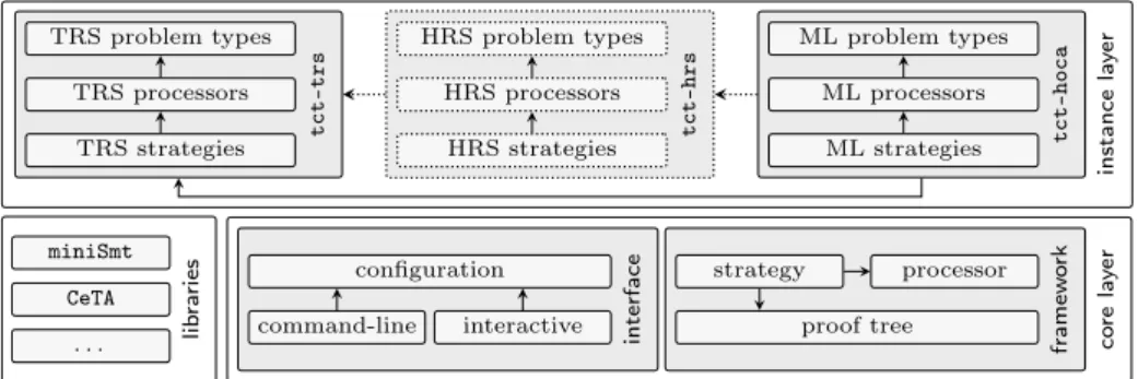
In this section we give an overview of the architecture of our complexity anal-yser. All components of TCT are written in the strongly typed, lazy functional programming language Haskell and released open source under BSD3. Our cur-rent code base consists of approximately 12.000 lines of code, excluding external libraries. The core constitutes roughly 17% of our code base, 78% of the code is dedicated to complexity techniques. The remaining 5% attribute to interfaces to external tools, such as CeTA5and SMT solvers, and common utility functions.
As depicted in Figure 1, the implementation of TCT is divided into separate components for the different program kinds and abstractions thereof supported. These separate components are no islands however. Rather, they instantiate our abstract complexity framework for complexity analysis [6], from which TCT de-rives its power and modularity. In short, in this framework complexity techniques are modelled as complexity processors that give rise to a set of inferences over complexity proofs. From a completed complexity proof, a complexity bound can be inferred. The theoretical foundations of this framework are given in Section 3. The abstract complexity framework is implemented in TCT’s core library, termed tct-core, which is depicted in Figure 2 at the bottom layer. Central,
5
configuration interface interactive command-line processor strategy framew o rk proof tree miniSmt CeTA . . . lib ra ries TRS strategies TRS processors TRS problem types tct-trs HRS strategies HRS processors HRS problem types tct-hrs ML strategies ML processors ML problem types tct-hoca co re la y er instance la y er
Fig. 2: Architectural Overview of TCT.
it provides a common notion of a proof state, viz proof trees, and an interface for specifying processors. Furthermore, tct-core complements the framework with a simple but powerful strategy language. Strategies play the role of tactics in interactive theorem provers like Isabelle or Coq. They allow us to turn a set of processors into a sophisticated complexity analyser. The implementation details of the core library are provided in Section 4.
The complexity framework implemented in our core library leaves the type of complexity problem, consisting of the analysed program together with the resource metric of interest, abstract. Rather, concrete complexity problems are provided by concrete instances, such as the two instances tct-hoca and tct-trs depicted in Figure 2. We will look at some particular instances in detail in Sec-tion 5. Instances implement complexity techniques on defined problem types in the form of complexity processors, possibly relying on external libraries and tools such as e.g. SMT solvers. Optionally, instances may also specify strate-gies that compose the provided processors. Bridges between instances are easily specified as processors that implement conversions between problem types de-fined in different instances. For example our instance tct-hoca, which deals with the runtime analysis of pure OCaml programs, makes use of the instance tct-trs. Thus our system is open to the seamless integration of alternative problem types through the specification of new instances. Exemplarily, we men-tion the envisioned instance tct-hrs (see Figure 1), which should incorporate dedicated techniques for the analysis of HRSs. We intend to use tct-hrs in future versions for the analysis of functional programs.
3
A Formal Framework for Complexity Analysis
We now briefly outline the theoretical framework upon which our complexity analyser TCT is based. As mentioned before, both the input language (e.g. Java, OCaml, . . . ) as well as the resource under consideration (e.g. execution time, heap usage, . . . ) is kept abstract in our framework. That is, we assume that we are dealing with an abstract class of complexity problems, where however, each complexity problem P from this class is associated with a complexity function
cpP : D → D, for a complexity domain D. Usually, the complexity domain D will be the set of natural numbers N, however, more sophisticated choices of complexity functions, such as e.g. those proposed by Danner et al. [11], fall into the realm of our framework.
In a concrete setting, the complexity problem P could denote, for instance, a Java program. If we are interested in heap usage, then D = N and cpP : N → N denotes the function that describes the maximal heap usage of P in the sizes of the program inputs. As indicated in the introduction, any transformational solver converts concrete programs into abstract ones, if not already interfaced with an abstract program. Based on the possible abstracted complexity problem P the analysis continues using a set of complexity techniques. In particular, a reasonable solver will also integrate some form of decomposition techniques, transforming an intermediate problem into various smaller sub-problems, and analyse these sub-problems separately, either again by some form of decomposition method, or eventually by some base technique which infers a suitable resource bound. Of course, at any stage in this transformation chain, a solver needs to keep track of computed complexity-bounds, and relay these back to the initial problem.
To support this kind of reasoning, it is convenient to formalise the internals of a complexity analyser as an inference system over complexity judgements. In our framework, a complexity judgement has the shape ` P : B, where P is a complexity problem and B is a set of bounding functions f : D → D for a complexity domain D. Such a judgement is valid if the complexity function of P lies in B, that is, cpP ∈ B. Complexity techniques are modelled as processors in our framework. A processor defines a transformation of the input problem P into a list of sub-problems Q1, . . . , Qn (if any), and it relates the complexity of the obtained sub-problems to the complexity of the input problem. Processors are given as inferences
P re(P) ` Q1: B1 · · · ` Qn: Bn ` P : B
,
where P re(P) indicates some pre-conditions on P. The processor is sound if under P re(P) the validity of judgements is preserved, i.e.
P re(P) ∧ cpQ1 ∈ B1∧ · · · ∧ cpQn∈ Bn =⇒ cpP ∈ B .
Dual, it is called complete if under the assumptions P re(P), validity of the judgement ` P : B implies validity of the judgements ` Qi: Bi.
A proof of a judgement ` P : B from the assumptions ` Q1: B1, . . . , ` Qn : Bn is a deduction using sound processors only. The proof is closed if its set of assumptions is empty. Soundness of processors guarantees that our formal system is correct. Application of complete processors on a valid judgement ensures that no invalid assumptions are derived. In this sense, the application of a complete processor is always safe.
Proposition 1. If there exists a closed complexity proof ` P : B, then the judgement ` P : B is valid.
4
Implementing the Complexity Framework
The formal complexity framework described in the last section is implemented in the core library, termed tct-core. In the following we outline the two central components of this library: (i) the generation of complexity proofs, and (ii) com-mon facilities for instantiating the framework to concrete tools, see Figure 2.
4.1 Proof Trees, Processors, and Strategies
The library tct-core provides the verification of a valid complexity judgement ` P : B from a given input problem P. More precise, the library provides the environment to construct a complexity proof witnessing the validity of ` P : B. Since the class B of bounding-functions is a result of the analysis, and not an input, the complexity proof can only be constructed once the analysis finished successfully. For this reason, proofs are not directly represented as trees over complexity judgements. Rather, the library features proof trees. Conceptually, a proof tree is a tree whose leaves are labelled by open complexity problems, that is, problems which remain to be analysed, and whose internal nodes represent successful applications of processors. The complexity analysis of a problem P then amounts to the expansion of the proof tree whose single node is labelled by the open problem P. Processors implement a single expansion step. To facilitate the expansion of proof trees, tct-core features a rich strategy language, similar to tactics in interactive theorem provers like Isabelle or Coq. Once a proof tree has been completely expanded, a complexity judgement for P together with the witnessing complexity proof can be computed from the proof tree.
In the following, we detail the central notions of proof tree, processor and strategy, and elaborate on important design issues.
Proof Trees: The first design issue we face is the representation of complexity problems. In earlier versions of TCT, we used a concrete problem typeProblem
that captured various notions of complexity problems, but all were based on term rewriting. With the addition of new kinds of complexity problem, such as runtime of functional or heap size of imperative programs, this approach be-came soon infeasible. In the present reimplementation, we therefore abstract over problem types, at the cost of slightly complicating central definitions. This allows concrete instantiations to precisely specify which problem types are sup-ported. Consequently, proof trees are parameterised in the type of complexity problems.
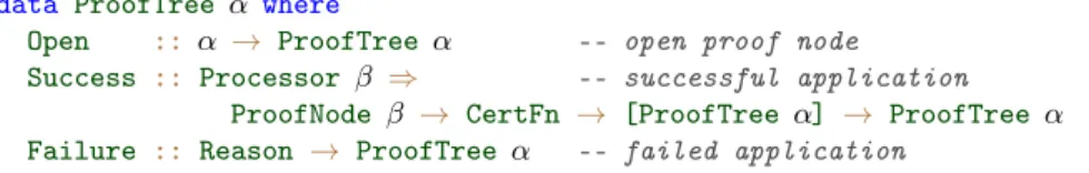
The corresponding (generalised) algebraic data-typeProofTree α(from mod-ule Tct.Core.Data.ProofTree) is depicted in Figure 3. A constructor Open rep-resents a leaf labelled by an open problem of typeα. The ternary constructor
Success represents the successful application of a processor of typeβ. Its first argument, a value of type ProofNodeβ, carries the applied processor, the cur-rent complexity problem under investigation as well as a proof-object of type
ProofObject β. This information is useful for proof analysis, and allows a de-tailed textual representation of proof trees. Note thatProofObjectis a type-level
data ProofTree α where
Open :: α → ProofTree α -- open proof node
Success :: Processor β ⇒ -- successful application
ProofNode β → CertFn → [ProofTree α] → ProofTree α
Failure :: Reason → ProofTree α -- failed application
Fig. 3: Data-type declaration of proof trees in tct-core.
function, the concrete representation of a proof-object thus depends on the type of the applied processor. The second argument toSuccessis a certificate-function
type CertFn =[Certificate] → Certificate,
which is used to relate the estimated complexity of generated sub-problems to the analysed complexity problem. Thus currently, the set of bounding-functions B occurring in the final complexity proof is fixed to those expressed by the data-typeCertificate(moduleTct.Core.Data.Certificate).Certificateincludes var-ious representations of complexity classes, such as the class of polynomials, ex-ponential, primitive and multiple recursive functions, but also the more fine grained classes of bounding-functions O(nk
) for all k ∈ N. The remaining ar-gument to the constructor Success is a forest of proof trees, each individual proof tree representing the continuation of the analysis of a corresponding sub-problem generated by the applied processor. Finally, the constructor Failure
indicates that the analysis failed. It results for example from the application of a processor to an open problem which does not satisfy the pre-conditions of the processor. The argument of type Reason allows a textual representation of the failure-condition. The analysis will always abort on proof trees containing such a failure node.
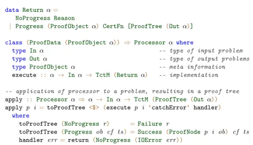
Processors. The interface for processors is specified by the type-classProcessor, which is defined in module Tct.Core.Data.Processor and depicted in Figure 4. The type of input problem and generated sub-problems are defined for processors on an individual basis, through the type-level functionsInandOut, respectively. This eliminates the need for a global problem type, and facilitates the seamless combination of different instantiations of the core library. Each processor in-stance specifies additionally the type of proof-objectsProofObject α– the meta information provided in case of a successful application. The proof-object is con-strained to instances of ProofData, which beside others, ensures that a textual representation can be obtained. Each instance of Processor has to implement a method execute, which given an input problem of type In α, evaluates to a
TctMaction that produces a value of typeReturn α. The monadTctM(defined in module Tct.Core.Data.TctM) extends the IO monad with access to runtime in-formation, such as command line parameters and execution time. The data-type
Return αspecifies the result of the application of a processor to its given input problem. In case of a successful application, the return value carries the proof-object, a value of typeCertFn, which relates complexity-bounds on sub-problems to bounds on the input-problem and the list of generated sub-problems. In fact
data Return α=
NoProgress Reason
| Progress (ProofObject α) CertFn [ProofTree (Out α)]
class (ProofData (ProofObject α)) ⇒ Processor α where
type In α -- type of input problem
type Out α -- type of output problems
type ProofObjectα -- meta information
execute :: α → In α → TctM (Return α) -- implementation -- application of processor to a problem, resulting in a proof tree
apply :: Processorα ⇒ α → In α → TctM (ProofTree (Out α))
apply p i =toProofTree <$> (execute p i ‘catchError‘ handler)
where
toProofTree (NoProgress r) =Failure r
toProofTree (Progress ob cf t s) =Success (ProofNode p i ob) cf t s handler err =return (NoProgress (IOError err))
Fig. 4: Data-type and class definitions related to processors in tct-core. the type is slightly more liberal and allows for each generated sub-problem a, possibly open, proof tree. This generalisation is useful in certain contexts, for example, when the processor makes use of a second processor.
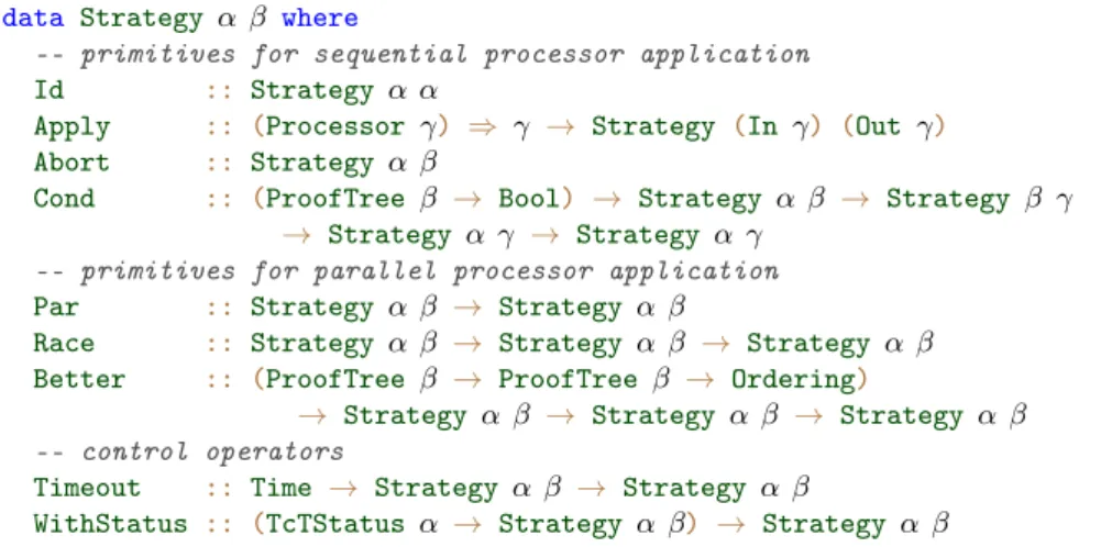
Strategies. To facilitate the expansion of a proof tree, tct-core features a simple but expressive strategy language. The strategy language is deeply embedded, via the generalised algebraic data-typeStrategy α βdefined in Figure 5. Semantics over strategies are given by the function
evaluate :: Strategy α β → ProofTree α → TctM (ProofTree β),
defined in moduleTct.Core.Data.Strategy. A strategy of typeStrategy α βthus translates a proof tree with open problems of typeαto one with open problems of typeβ.
The first four primitives defined in Figure 5 constitute our tool box for mod-elling sequential application of processors. The strategy Id is implemented by the identity function on proof trees. The remaining three primitives traverse the given proof tree in-order, acting on all the open proof-nodes. The strategy
Apply p replaces the given open proof-node with the proof tree resulting from an application of p. The strategyAbort signals that the computation should be aborted, replacing the given proof-node by a failure node. Finally, the strategy
Cond predicate s1 s2 s3implements a very specific conditional. It sequences the application of strategiess1ands2, provided the proof tree computed bys1 sat-isfies the predicatepredicate. For the case where the predicate is not satisfied, the conditional acts like the third strategys3.
In Figure 6 we showcase the definition of derived sequential strategy com-binators. Sequencings1 ≫ s2of strategiess1ands2as well as a (left-biased) choice operators1 <|> s2are derived from the conditional primitiveCond. The
data Strategy α β where
-- primitives for sequential processor application
Id :: Strategy α α
Apply :: (Processor γ) ⇒ γ → Strategy (In γ) (Out γ)
Abort :: Strategy α β
Cond :: (ProofTree β → Bool) → Strategy α β → Strategy β γ
→ Strategy α γ → Strategy α γ
-- primitives for parallel processor application
Par :: Strategy α β → Strategy α β
Race :: Strategy α β → Strategy α β → Strategy α β
Better :: (ProofTree β → ProofTree β → Ordering)
→ Strategy α β → Strategy α β → Strategy α β
-- control operators
Timeout :: Time → Strategy α β → Strategy α β
WithStatus :: (TcTStatus α → Strategy α β) → Strategy α β
Fig. 5: Deep Embedding of our strategy language in tct-core.
strategy try s behaves like s, except when s fails then try s behaves as an identity. The combinator force complements the combinator try: the strategy
force s enforces that strategy s produces a new proof-node. The combinator
trybrings backtracking to our strategy language, i.e. the strategytry s1 ≫ s2
first applies strategys1, backtracks in case of failure, and appliess2afterwards.
Finally, the strategiesexhaustive sappliesszero or more times, until strategys
fails. The combinatorexhaustive+behaves similarly, but applies the given strat-egy at least once. The obtained combinators satisfy the expected laws, compare Figure 7 for an excerpt.
Our strategy language features also three dedicated types for parallel proof search. The strategyPar simplements a form of data level parallelism, applying strategy sto all open problems in the given proof tree in parallel. In contrast, the strategies Race s1 s2 and Better comp s1 s2 apply to each open problem the strategies s1 and s2 concurrently, and can be seen as parallel version of our choice operator. WhereasRace s1 s2simply returns the (non-failing) proof tree of whichever strategy returns first, Better comp s1 s2 uses the provided
comparison-functioncompto decide which proof tree to return.
The final two strategies depicted in Figure 5 implement timeouts, and the dynamic creation of strategies depending on the current TctStatus. TctStatus
includes global state, such as command line flags and the execution time, but also proof relevant state such as the current problem under investigation.
4.2 From the Core to Executables
The framework is instantiated by providing a set of sound processors, together with their corresponding input and output types. At the end of the day the complexity framework has to give rise to an executable tool, which, given an initial problem, possibly provides a complexity certificate.
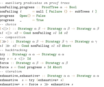
-- auxiliary predicates on proof trees
nonFailing,progress :: ProofTree α → Bool
nonFailing t =null [ Failure {} ← subTrees t ]
progress Open{} =False
progress _ =True
-- choice
(<|>) :: Strategy α β → Strategy α β → Strategy α β s1 <|> s2=Cond nonFailing s1 Id s2
-- composition
(≫) :: Strategy α β → Strategy β γ → Strategy α γ s1 ≫ s2 =Cond nonFailing s1 s2 Abort
-- backtracking
try :: Strategy α α → Strategy α α try s =s <|> Id
force :: Strategy α β → Strategy α β force s =Cond progress s Id Abort
-- iteration
exhaustive,exhaustive+ :: Strategy α α → Strategy α α exhaustive s=try (exhaustive+ s)
exhaustive+ s =force s ≫ exhaustive s
Fig. 6: Derived sequential strategy combinators.
To ease the generation of such an executable, tct-core provides a default implementation of themainfunction, controlled by aTctConfigrecord (see mod-ule Tct.Core.Main). A minimal definition of TctConfigjust requires the
speci-fication of a default strategy, and a parser for the initial complexity problem. Optionally, one can for example specify additional command line parameters, or a list of declarations for custom strategies, which allow the user to control the proof search. Strategy declarations wrap strategies with additional meta information, such as a name, a description, and a list of parameters. Firstly, this information is used for documentary purposes. If we call the default im-plementation with the command line flag –-list-strategies it will present a documentation of the available processors and strategies to the user. Secondly, declarations facilitate the parser generation for custom strategies. It is notewor-thy to mention that declarations and the generated parsers are type safe and are checked during compile-time. Declarations, together with usage information, are defined in moduleTct.Core.Data.Declaration. Given a path pointing to the file holding the initial complexity problem, the generated executable will perform the following actions in order:
1. Parse the command line options given to the executable, and reflect these in the aforementionedTctStatus.
2. Parse the given file according to the parser specified in the TctConfig. 3. Select a strategy based on the command line flags, and apply the selected
strategy on the parsed input problem.
4. Should the analysis succeed, a textual representation of the obtained com-plexity judgement and corresponding proof tree is printed to the console; in
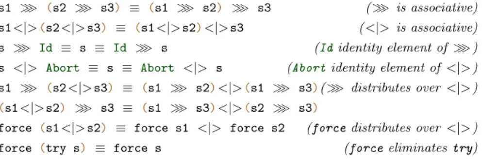
s1 ≫ (s2 ≫ s3) ≡ (s1 ≫ s2) ≫ s3 (≫ is associative) s1 <|>(s2 <|> s3) ≡ (s1 <|> s2)<|> s3 ( <|> is associative) s ≫ Id ≡ s ≡ Id ≫ s (Ididentity element of ≫ ) s <|> Abort ≡ s ≡ Abort <|> s (Abortidentity element of <|> ) s1 ≫ (s2 <|> s3) ≡ (s1 ≫ s2)<|>(s1 ≫ s3)(≫ distributes over <|> )
(s1 <|> s2) ≫ s3 ≡ (s1 ≫ s3)<|>(s2 ≫ s3)
force (s1 <|> s2) ≡ force s1 <|> force s2 (force distributes over <|> ) force (try s) ≡ force s (force eliminates try)
Fig. 7: Some laws obeyed by the derived operators.
case the analysis fails, the uncompleted proof tree, including theReason for failure is printed to the console.
Interactive. The library provides an interactive mode via the GHCi interpreter, similar to the one provided in TCT v2 [5]. The interactive mode is invoked via the command line flag –-interactive. The implementation keeps track of a proof state, a list of proof trees that represents the history of the interactive session. We provide an interface to inspect and manipulate the proof state. Most noteworthy, the user can select individual sub-problems and apply strategies on them. The proof state is updated accordingly.
5
Case Studies
In this section we discuss several instantiations of the framework that have been established up to now. We keep the descriptions of the complexity problems in-formal and focus on the big picture. In the discussion we group abstract programs in contrast to real world programs.
5.1 Abstract Programs
Currently TCT provides first-order term rewrite systems and integer transition systems as abstract representations. As mentioned above, the system is open to the seamless integration of alternative abstractions.
Term Rewrite Systems. Term rewriting forms an abstract model of computation, which underlies much of declarative programming. Our results on pure OCaml, see below, show how we can make practical use of the clarity of the model. The tct-trs instance provides automated resource analysis of first-order term rewrite systems (TRSs for short) [8,26]. Complexity analysis of TRSs has re-ceived significant attention in the last decade, see [19] for details. A TRS consists of a set of rewrite rules, i.e. directed equations that can be applied from left to right. Computation is performed by normalisation, i.e. by successively applying rewrite rules until no more rules apply. As an example, consider the following
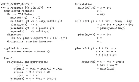
WORST_CASE(?,O(n^2)) *** 1 Progress [(?,O(n^2))] *** Considered Problem: Strict TRS Rules: mult(0(),y) -> 0() mult(s(x),y) -> plus(y,mult(x,y)) plus(x,0()) -> x plus(s(x),y) -> s(plus(x,y)) square(x) -> mult(x,x) Signature: {mult/2,plus/2,square/1} / {0/0,s/1} Obligation: runtime innermost Applied Processor:
NaturalPI {shape = Mixed 2} Proof: Polynomial Interpretation: p(0) = 1 p(mult) = 3*x1 + 2*x1*x2 + 2*x2 p(plus) = 2 + 2*x1 + x2 p(s) = 1 + x1 p(square) = 6 + 7*x1 + 2*x1^2 Orientation: mult(0(),y) = 3 + 4*y > 1 = 0()
mult(s(x),y) = 3 + 3*x + 2*x*y + 4*y > 2 + 3*x + 2*x*y + 4*y = plus(y,mult(x,y)) plus(x,0()) = 3 + 2*x > x = x plus(s(x),y) = 4 + 2*x + y > 3 + 2*x + y = s(plus(x,y)) square(x) = 6 + 7*x + 2*x^2 > 5*x + 2*x^2 = mult(x,x)
Fig. 8: Polynomial Interpretation Proof.
TRS Rsq, which computes the squaring function on natural numbers in unary notation.
sq(x) → x ∗ x x ∗ 0 → 0 x + 0 → x
s(x) ∗ y → y + (x ∗ y) s(x) + y → s(x + y) . The runtime complexity of a TRS is naturally expressed as a function that mea-sures the length of the longest reduction, in the sizes of (normalised) starting terms. Figure 8 depicts the proof output of tct-trs when applying a polyno-mial interpretation [18] processor with maximum degree 2 on Rsq. The resulting proof tree consists of a single progress node and returns the (optimal) quadratic asymptotic upper bound on the runtime complexity of Rsq. The success of TCT as a complexity analyser, and in particular the strength of tct-trs instance is apparent from its performance at TERMCOMP.6 It is noteworthy to men-tion that at this year’s competimen-tion TCT not only won the combined ranking, but also the certified category. Here only those techniques are admissible that have been machine checked, so that soundness of the obtained resource bound is almost without doubt, cf. [7]. The tct-trs instance has many advantages in comparison to its predecessors. Many of them are subtle and are due to the redesign of the architecture and reimplementation of the framework. However, the practical consequences are clear: the instance tct-trs is more powerful than its predecessor, cf. the last year’s TERMCOMP, where both the old and new version competed against each other. Furthermore, the actual strength of the latest version of TCT shows when combining different modules into bigger ones, as we are going to show in the sequent case studies.
6
Integer Transition Systems. The tct-its module deals with the analysis of integer transition systems (ITSs for short). An ITS can be seen as a TRS over terms f(x1, . . . , xn) where the variables xi range over integers, and where rules are additionally equipped with a guardJ·K that determines if a rule triggers. The notion of runtime complexity extends straight forward from TRSs to ITSs. ITSs naturally arise from imperative programs using loops, conditionals and integer operations only, but can also be obtained from programs with user-defined data structures using suitable size-abstractions (see e.g. [22]). Consider the following program, that computes the remainder of a natural number m with respect to n.
int rem(int m,int n){ while(n > 0 && m > n){ m = m - n }; return m; }
This program is represented as the following ITS:
r(m, n) → r(m − n, n)Jn > 0 ∧ m > nK r(m, n) → e(m, n)J¬(n > 0 ∧ m > n)K . It is not difficult to see that the runtime complexity of the ITS, i.e. the maximal length of a computation starting from r(m, n), is linear in m and n. The linear asymptotic bound is automatically derived by tct-its, in a fraction of a second. The complexity analysis of ITSs implemented by tct-its follows closely the approach by Brockschmidt et al. [10].
5.2 Real World Programs
One major motivation for the complexity analysis of abstract programs is that these models are well equipped to abstract over real-world programs whilst re-maining conceptually simple.
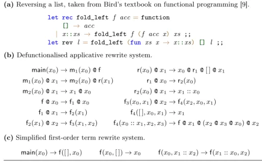
Pure OCaml. For the case of higher-order functional programs, a successful ap-plication of this has been demonstrated in recent work by the first and second author in collaboration with Dal Lago [4]. In [4], we study the runtime complex-ity of pure OCaml programs. A suitable adaption of Reynold’s defunctionalisa-tion [24] technique translates the given program into a slight generalisadefunctionalisa-tion of TRSs, an applicative term rewrite system (ATRS for short). In ATRSs closures are explicitly represented as first-order structures. Evaluation of these closures is defined via a global apply function (denoted by @).
The structure of the defunctionalised program is necessarily intricate, even for simple programs. However, in conjunction with a sequence of sophisticated and in particular complexity reflecting transformations one can bring the de-functionalised program in a form which can be effectively analysed by first-order complexity provers such as the tct-trs instance; see [4] for the details. An example run is depicted in Figure 9. All of this has been implemented in a prototype implementation, termed HoCA.7 We have integrated the functional-ity of HoCA in the instance tct-hoca. The individual transformations underly-ing this tool are seamlessly modelled as processors, its transformation pipeline is naturally expressed in our strategy language. The corresponding strategy,
7
(a) Reversing a list, taken from Bird’s textbook on functional programming [9]. let rec fold_left f acc=function
[] → acc
| x::xs → fold_left f (f acc x) xs ;;
let rev l =fold_left (fun xs x → x::xs) [] l ;; (b) Defunctionalised applicative rewrite system.
main(x0) → m1(x0) @ f r(x0) @ x1→ x0@ r1@ [ ] @ x1 m1(x0) @ x1→ m2(x0) @ r(x1) r1@ x0→ r2(x0) m2(x0) @ x1→ x1 @ x0 r2(x0) @ x1→ x1:: x0 f @ x0→ f1@ x0 f3(x0, x1) @ x2→ f4(x2, x0, x1) f1@ x1→ f2(x1) f4([ ], x0, x1) → x1 f2(x1) @ x2→ f3(x1, x2) f4(x0:: x1, x2, x3) → f @ x1 @ (x2@ x3@ x0) @ x2
(c) Simplified first-order term rewrite system.
main(x0) → f([ ], x0) f(x0, [ ]) → x0 f(x0, x1:: x2) → f(x1:: x0, x2)
Fig. 9: Example run of the HoCA prototype on a OCaml program.
hoca :: Maybe String → Strategy ML TrsProblem
hoca name=mlToAtrs name ≫ atrsToTrs ≫ toTctProblem mlToAtrs :: Maybe String → Strategy ML ATRS
mlToAtrs name=mlToPcf name ≫ defunctionalise ≫ try simplifyAtrs atrsToTrs :: Strategy ATRS TRS
atrsToTrs=try cfa ≫ uncurryAtrs ≫ try simplifyTrs
Fig. 10: HoCA transformation pipeline modelled in tct-hoca.
termed hoca, is depicted in Figure 10. It takes an OCaml source fragment, of typeML, and turns it into a term rewrite system as follows. First, viamlToAtrs
the source code is parsed and desugared, the resulting abstract syntax tree is turned into an expression of a typed λ-calculus with constants and fixpoints, akin to Plotkin’s PCF [23]. All these steps are implemented via the strat-egy mlToPcf :: Maybe String → Strategy ML TypedPCF. The given parameter, an optional function name, can be used to select the analysed function. With
defunctionalise :: Strategy TypedPCF ATRSthis program is then turned into an ATRS, which is simplified via the strategysimplifyAtrs :: Strategy ATRS ATRS
modelling the heuristics implemented in HoCA. Second, the strategy atrsToTrs
uses the control-flow analysis provided by HoCA to instantiate occurrences of higher-order variables [4]. The instantiated ATRS is then translated into a first-order rewrite system by uncurrying all function calls. Further simplifications, as foreseen by the HoCA prototype at this stage of the pipeline, are performed via the strategysimplifyTrs :: Strategy TRS TRS.
jbc :: Strategy ITS () → Strategy TRS () → Strategy JBC ()
jbc its trs=toCTRS ≫ Race (toIts ≫ its) (toTrs ≫ trs)
Fig. 11: jat transformation pipeline modelled in tct-jbc.
Currently, all involved processors are implemented via calls to the library shipped with the HoCA prototype, and operate on exported data-types. The fi-nal strategy in the pipeline,toTctProblem :: Strategy TRS TrsProblem, converts HoCA’s representation of a TRS to a complexity problem understood by tct-trs. Due to the open structure of TCT, the integration of the HoCA prototype worked like a charm and was finalised in a couple of hours. Furthermore, essentially by construction the strength of tct-hoca equals the strength of the dedicated prototype. An extensive experimental assessment can be found in [4].
Object-Oriented Bytecode Programs. The tct-jbc instance provides automated complexity analysis of object-oriented bytecode programs, in particular Jinja bytecode (JBC for short) programs [17]. Given a JBC program, we measure the maximal number of bytecode instructions executed in any evaluation of the program. We suitably employ techniques from data-flow analysis and abstract interpretation to obtain a term based abstraction of JBC programs in terms of constraint term rewrite systems (cTRSs for short) [20]. CTRSs are a generalisa-tion of TRSs and ITSs. More importantly, given a cTRS obtained from a JBC program, we can extract a TRS or ITS fragment. All these abstractions are com-plexity reflecting. We have implemented this transformation in a dedicated tool termed jat and have integrated its functionality in tct-jbc in a similar way we have integrated the functionality of HoCA in tct-hoca. The corresponding strategy, termed jbc, is depicted in Figure 11. We then can use tct-trs and
tct-its to analyse the resulting problems. Our framework is expressive enough to analyse the thus obtained problems in parallel. Note thatRace s1 s2requires that s1 and s2 have the same output problem type. We can model this with transformations to a dummy problem (). Nevertheless, as intended any witness that is obtained by an successful application of itsortrswill be relayed back.
6
Conclusion
In this paper we have presented TCT v3.0, the latest version of our fully auto-mated complexity analyser. TCT is open source, released under the BSD3 license. All components of TCT are written in Haskell. TCT is open with respect to the complexity problem under investigation and problem specific techniques. It is the most powerful tool in the realm of automated complexity analysis of term rewrite systems, as for example verified at this year’s TERMCOMP. Moreover it provides an expressive problem independent strategy language that facilitates the proof search, extensibility and automation.
Further work will be concerned with the finalisation of the envisioned instance tct-hrs, as well as the integration of current and future developments in the resource analysis of ITSs.
References
1. Albert, E., Arenas, P., Genaim, S., Puebla, G., Román-Díez, G.: Conditional Ter-mination of Loops over Heap-allocated Data. SCP 92, 2–24 (2014)
2. Aspinall, D., Beringer, L., Hofmann, M., Loidl, H.W., Momigliano, A.: A Program Logic for Resources. TCS 389(3), 411–445 (2007)
3. Atkey, R.: Amortised Resource Analysis with Separation Logic. LMCS 7(2) (2011) 4. Avanzini, M., Lago, U.D., Moser, G.: Analysing the Complexity of Functional Pro-grams: Higher-Order Meets First-Order. In: Proc. 20th ICFP. ACM (2015), to appear
5. Avanzini, M., Moser, G.: Tyrolean Complexity Tool: Features and Usage. In: Proc. of 24th RTA. LIPIcs, vol. 21, pp. 71–80 (2013)
6. Avanzini, M., Moser, G.: A Combination Framework for Complexity. IC (2016), to appear
7. Avanzini, M., Sternagel, C., Thiemann, R.: Certification of Complexity Proofs using CeTA. In: Proc. of 26th RTA. LIPIcs, vol. 36, pp. 23–39 (2015)
8. Baader, F., Nipkow, T.: Term Rewriting and All That. Cambridge University Press (1998)
9. Bird, R.: Introduction to Functional Programming using Haskell, Second Edition. Prentice Hall (1998)
10. Brockschmidt, M., Emmes, F., Falke, S., Fuhs, C., Giesl, J.: Alternating Runtime and Size Complexity Analysis of Integer Programs. In: Proc. 20th TACAS. pp. 140–155. LNCS (2014)
11. Danner, N., Paykin, J., Royer, J.S.: A Static Cost Analysis for a Higher-order Language. In: Proc. of 7th PLPV. pp. 25–34. ACM (2013)
12. Gimenez, S., Moser, G.: The Complexity of Interaction. In: Proc. of 40th POPL (2016), to appear
13. Hirokawa, N., Moser, G.: Automated Complexity Analysis Based on the Depen-dency Pair Method. In: Proc. 4th IJCAR. LNCS, vol. 5195, pp. 364–380 (2008) 14. Hoffmann, J., Aehlig, K., Hofmann, M.: Multivariate Amortized Resource Analysis.
TOPLAS 34(3), 14 (2012)
15. Hofmann, M., Moser, G.: Multivariate Amortised Resource Analysis for Term Rewrite Systems. In: Proc. 13th TLCA. pp. 241–256. No. 38 in LIPIcs (2015) 16. Jost, S., Hammond, K., Loidl, H.W., Hofmann, M.: Static Determination of
Quan-titative Resource Usage for Higher-order Programs. In: Proc. of 37th POPL. pp. 223–236. ACM (2010)
17. Klein, G., T-Nipkow: A Machine-Checked Model for a Java-like Language, Virtual Machine, and Compiler. TOPLAS 28(4), 619–695 (2006)
18. Lankford, D.: On Proving Term Rewriting Systems are Noetherian. Tech. Rep. MTP-3, Louisiana Technical University (1979)
19. Moser, G.: Proof Theory at Work: Complexity Analysis of Term Rewrite Systems. CoRR abs/0907.5527 (2009), Habilitation Thesis
20. Moser, G., Schaper, M.: A Complexity Preserving Transformation from Jinja Byte-code to Rewrite Systems. CoRR, cs/PL/1204.1568 (2012), last revision: May 6, 2014
21. Noschinski, L., Emmes, F., Giesl, J.: Analyzing Innermost Runtime Complexity of Term Rewriting by Dependency Pairs. JAR 51(1), 27–56 (2013)
22. P. M. Hill, E. Payet and F. Spoto: Path-length Analysis of Object-Oriented Pro-grams. In: In Proc. 1st EAAI. Elsevier (2006)
23. Plotkin, G.D.: LCF Considered as a Programming Language. TCS 5(3), 223–255 (1977)
24. Reynolds, J.C.: Definitional Interpreters for Higher-Order Programming Lan-guages. HOSC 11(4), 363–397 (1998)
25. Sinn, M., Zuleger, F., Veith, H.: A Simple and Scalable Static Analysis for Bound Analysis and Amortized Complexity Analysis. In: Proc. 26th CAV. pp. 745–761 (2014)
26. TeReSe: Term Rewriting Systems, Cambridge Tracks in Theoretical Computer Science, vol. 55. Cambridge University Press (2003)
27. Wilhelm, R., Engblom, J., Ermedahl, A., Holsti, N., Thesing, S., Whalley, D., Bernat, G., Ferdinand, C., Heckmann, R., Mitra, T., Mueller, F., Puaut, I., Puschner, P., Staschulat, J., Stenstrom, P.: The Worst Case Execution Time Prob-lem - Overview of Methods and Survey of Tools. TECS 7(3), 1–53 (2008)