HAL Id: hal-01806169
https://hal.archives-ouvertes.fr/hal-01806169
Submitted on 27 Oct 2020HAL is a multi-disciplinary open access archive for the deposit and dissemination of sci-entific research documents, whether they are pub-lished or not. The documents may come from teaching and research institutions in France or abroad, or from public or private research centers.
L’archive ouverte pluridisciplinaire HAL, est destinée au dépôt et à la diffusion de documents scientifiques de niveau recherche, publiés ou non, émanant des établissements d’enseignement et de recherche français ou étrangers, des laboratoires publics ou privés.
Full-Waveform Lidar Onboard a Satellite Initialized
from Airborne Ultraviolet Lidar Experiments
Xiaoxia Shang, Patrick Chazette
To cite this version:
Xiaoxia Shang, Patrick Chazette. End-to-End Simulation for a Forest-Dedicated Full-Waveform Lidar Onboard a Satellite Initialized from Airborne Ultraviolet Lidar Experiments. Remote Sensing, MDPI, 2015, 7 (5), pp.5222 - 5255. �10.3390/rs70505222�. �hal-01806169�
remote sensing
ISSN 2072-4292www.mdpi.com/journal/remotesensing Article
End-to-End Simulation for a Forest-Dedicated Full-Waveform
Lidar Onboard a Satellite Initialized from Airborne Ultraviolet
Lidar Experiments
Xiaoxia Shang * and Patrick Chazette
Laboratoire des Sciences du Climat et l’Environnement, Commissariat à l’Energie Atomique et aux Energies Alternatives—Centre National de la Recherche Scientifique—Université de Versailles Saint-Quentin-en-Yvelines, Gif sur Yvette Cedex 91191, France; E-Mail: patrick.chazette@lsce.ipsl.fr
* Author to whom correspondence should be addressed; E-Mail: xiaoxia.shang@gmail.com;
Tel.: +33-1-6908-7889; Fax: +33-1-6908-7716.
Academic Editors: Peter Krzystek, Wei Yao, Yong Pang, Marco Heurich and Prasad S. Thenkabail Received: 11 February 2015 / Accepted: 20 April 2015 / Published: 27 April 2015
Abstract: In order to study forests at the global scale, a detailed link budget for a lidar system
onboard satellite is presented. It is based on an original approach coupling airborne lidar observations and an end-to-end simulator. The simulator is initialized by airborne lidar measurements performed over temperate and tropical forests on the French territory, representing a wide range of forests ecosystems. Considering two complementary wavelengths of 355 and 1064 nm, the end-to-end simulator computes the performance of spaceborne lidar systems for different orbits. The analysis is based on forest structural (tree top height, quadratic mean canopy height) and optical (forest optical thickness) parameters. Although an ultraviolet lidar appears to be a good candidate for airborne measurements, our results show that the limited energy is not favorable for spaceborne missions with such a wavelength. A near infrared wavelength at 1064 nm is preferable, requiring ~100 mJ laser emitted energy, which is in agreement with current and future spaceborne missions involving a lidar. We find that the signal-to-noise ratio at the ground level to extract both the structural and optical parameters of forests must be larger than 10. Hence, considering the presence of clouds and aerosols in the atmosphere and assuming a stationary forest, a good detection probability of 99% can be reached when 4 or 5 satellite revisits are considered for a lidar system onboard the ISS or ICESat, respectively. This concerns ~90% of forest covers observed from the lidar, which have an optical thickness less than 3.
Keywords: link budget; spaceborne; canopy; lidar; simulation
1. Introduction
Forests are key components of surface-atmosphere interactions as demonstrated by previous studies [1–5]. They are sinks or sources for many atmospheric compounds that play major roles on the atmospheric chemistry such as the ozone cycle and the secondary organic aerosol formation [6–9]. Representing 80% of the continental biosphere carbon stock, forests also sequester large carbon dioxide from the atmosphere [9] and act as conservators of the biodiversity [10,11]. The biodiversity of forests depend on the three-dimensional (3D) distribution of canopy structures, which contains a substantial amount of information about the state of development of plant communities [12–16]. However the 3D canopy structures are not yet available at the global scale until now. Spaceborne observation, including passive and active remote sensing systems, is a good approach to get such information of canopy structures. Passive multispectral and hyper-spectral sensors produce two-dimensional atmosphere/ground information, whereas their ability to represent 3D spatial patterns is limited. For instance, their use for tropical dense forests is not adequate because the remote sensor has difficulty to penetrate the upper canopy layer [17]. On the other hand, active sensors, including lidar and radar, have been shown to be valuable tools for 3D vegetation mapping and characterization. Recent developments in P-band radar technology and data processing techniques allow accurate estimates with a large spectrum of forest biomass [18–20]. For instance, the BIOMASS Earth Explorer mission selected by ESA in the framework of its Living Planet program is envisaged as a P-band spaceborne Synthetic Aperture Radar (SAR) satellite. This future space mission aims at providing consistent global estimates of the forest biomass, disturbances and re-growth. However, radar gives more information about the volume and is less efficient to restitute the forest vertical structure than lidar. Lidar therefore appears to be a complementary instrument for both short and medium-term spaceborne missions in the future.
Previous studies have been performed to evaluate the potential of spaceborne lidar systems [21–24]. Nevertheless, these authors did not take into account the orbits and the related atmospheric contribution in their studies. Moreover, the instrumental characteristics were not explicitly analyzed. A spaceborne backscatter lidar could provide a full description of the forest vertical structures [25], and forest dynamics resulting from deforestation (clear-cut), forest management, or climate change [26–28]. Lidar technology is now very mature, as demonstrated by the LITE experiment [29], the operational CALIPSO mission [30,31], and the ICESat mission [32]. Furthermore, the MOLI (Multi-Footprint Observation LiDAR and Imager) project selected by JAXA [33] and the GEDI (Global Ecosystem Dynamics Investigation Lidar) project selected by NASA [34] would involve embedding on the International Space Station (ISS) a vegetation lidar system for forest studies. A large-footprint lidar (a few tens of meters’ footprint at the ground level) can accurately map canopy structures and aboveground biomass [35–40], even in high-biomass ecosystems where passive optical and active radar sensors typically fail to do so.
In this paper, a detailed link budget for a canopy lidar system onboard satellite is presented. It complements the previously published works [21,22], by using an original approach coupling airborne lidar observations and an end-to-end simulator. This work has been conducted based on field experiments
specifically conducted over French forests between 2008 and 2014. It aims at a pre-feasibility study of a spaceborne lidar dedicated to forest survey, required before a future Assessment Phase (Phase-0) by the Centre National d’Etude Spatial (CNES).
In Section 2, we present our semi-empirical approach, by describing the end-to-end simulator (including the direct and inverse models), the sampling sites, and the adjustment of parameters. In Section 3, using the end-to-end modeling in ultraviolet (UV) and near infrared (NIR) wavelengths, the footprint size, the optimal signal-to-noise ratio (SNR), and the signal distortion are discussed in detail. In Section 4, the link budget for several platforms is presented for the two selected wavelengths (355 and 1064 nm). The atmospheric scattering properties and the orbital configuration are also considered in our numerical simulations.
2. Methodology
2.1. Overview
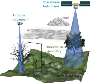
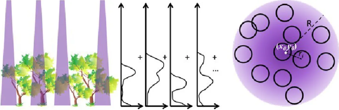
The modeling of the lidar signal can be achieved based on a semi-empirical approach using the airborne lidar measurements and the radiative transfer equation applied to the laser beam propagation into a scattering medium (leaves, branches, trunks). The lidar instrument ULICE (Ultraviolet LIdar for Canopy Experiment) was embedded on an Ultra-Light Aircraft (ULA) (Figure 1) as for previous atmospheric [41] and canopy [25] studies. It performed airborne measurements over different forest biomes between 2008 and 2014, from temperate to tropical forests, to obtain a representative database of lidar vertical profiles. This database is used to initialize analytical and statistical modeling of the lidar signal, so as to simulate spaceborne observations.
Figure 1. Illustration of airborne and spaceborne lidar measurements.
The canopy lidar or topographic lidar typically use wavelengths in the near infrared (NIR, i.e., 1064 nm), which corresponds to the fundamental emission of a commercial solid-state Nd:YAG laser. However, we will show that there are significant multiple scattering (MS) effects on the retrieval of
forest structures at this wavelength, because of the high reflectance of the vegetation. These effects distort the lidar profile and make it difficult to locate the ground echo (GE) and the canopy echo (CE). Doubling the fundamental frequency, the Nd:YAG laser emits at 532 nm but it is quite difficult to get the eye-safe condition with such a wavelength. Thus, a laser operating at an ultraviolet (UV) wavelength (355 nm) was used in our airborne lidar measurements, which is available with the Nd:YAG laser using a non-linear crystal by tripling the fundamental frequency. The use of the UV spectral domain leads to a significant reduction of the MS effects in the forest structures and relaxes the constraints for operating eye-safety measurements.
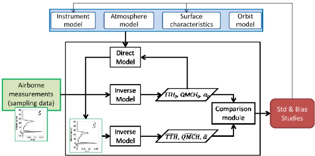
In order to characterize a forest site, three key parameters were derived from lidar backscatter profiles: (1) tree top height (TTH), a basic parameter for forest studies which is calculated as the distance between the first return at the upper surface of the vegetation and the last return of the ground surface [25,42]; (2) quadratic mean canopy height (QMCH), a structural parameter which can be used to evaluate the aboveground biomass [15,42]; (3) extinction coefficient (α), an optical property indicating forest characteristics (e.g., canopy density and forest category) closely related to the forest optical thickness (FOT). All the structural and optical parameters are linked to the lidar equation as shown in Section 2.2. An end-to-end simulator (EES) was specifically developed for this study, which is a powerful tool to simulate and analyze the performance of airborne and spaceborne lidar systems. It is composed of a direct model and an inverse model. The block diagram of EES is shown in Figure 2. From airborne lidar measurements (e.g., lidar profile S), forest parameters (i.e., TTH0, QMCH0, α0 in Figure 2) can be derived
from the inverse model so as to initialize the direct model. Meanwhile, four types of external data (in the blue bloc of Figure 2) were used to provide additional necessary constraints to the direct model: (1) an instrument model, including instrumental parameters of the lidar system and related uncertainties; (2) an atmosphere model, which includes the atmospheric contributions (i.e., molecular, aerosol and cloud optical thickness); (3) surface characteristics, which provide the necessary surface information and identify forest and non-forest areas as well as forest types at the global scale; (4) an orbit model, in order to simulate the different possible orbits for spaceborne lidar systems.
Lidar vertical profiles were simulated by the direct model. The main sources of noise were taken into account considering normal statistical distributions. Next, estimated forest parameters (i.e., 𝑇𝑇𝐻̃, 𝑄𝑀𝐶𝐻̃ , 𝛼̃ in Figure 2) for each simulated lidar profile (𝑆̃) were derived by the inverse model. The comparison between these estimated parameters and the initial values presented as inputs of the direct model was then performed in the “comparison module”. The assessments of the standard deviation and bias of each parameter, and of the related signal-to-noise ratio (SNR), have been done following a Monte Carlo approach [43]. For each statistical simulation we used 200 statistical draws which thus ensured a normal distribution around the mean values. The main components of the EES will be detailed below.
Figure 2. Block diagram of the end-to-end simulator. Both the standard deviations and the
bias of the tree top height (TTH), the quadratic mean canopy height (QMCH) and the extinction coefficient (α) are computed using a Monte Carlo approach. TTH0, QMCH0 and
α0 are initial values derived from the real lidar signal S. 𝑇𝑇𝐻̃, 𝑄𝑀𝐶𝐻̃ and 𝛼̃ are estimated
values derived from the simulated lidar profile 𝑆̃ for each statistical draw. 2.2. Direct Model
Lidar signals from both air- or space-platform can be expressed by the lidar equation [44]. The backscattered lidar signal Sv above the ground, for a nadir measurement taken at a height above ground
level (agl) h in the forest (with a ground altitude zground) and a wavelength λ, is given by [44]:
𝑆𝑣(𝜆, ℎ) ≈ 𝐾(𝜆) ∙ 𝐸(𝜆) ∙ 1 (𝑍𝑝− (ℎ + 𝑧𝑔𝑟𝑜𝑢𝑛𝑑)) 2∙ 𝐵𝐸𝑅(𝜆, ℎ) ∙ 𝛼𝐹𝑂𝑇(𝜆, ℎ) ∙ exp [−2 (𝐹𝑂𝑇(ℎ) 2 ∙ 𝜂(𝜆, ℎ) + 𝜏(ℎ))] (1)
where we supposed that the atmospheric backscattered part in the canopy is negligible compared to the larger backscattered part of the canopy. The instrumental constant K (λ) and the laser energy E(λ) are defined in the “instrument model” (Section 2.2.1, Equation (3)). FOT is the forest optical thickness (cf. Section 2.3) and τ is the total atmospheric optical thickness as defined in the “Atmosphere model” (Section 2.2.2). The backscatter to extinction ratio BER (λ, h) and the multiple scattering coefficient η are defined in the “Surface characteristics” (Section 2.2.3). The BER, which is linked to tree species, can be also interpreted as the probability of photons backscattered after the interaction of the laser beam and the forest materials. Zp is the altitude agl of the platform, which is defined in Section 2.2.4. The
canopy extinction coefficient αFOT (λ, h) is defined as the sum of the absorption and scattering
coefficients, which can be obtained from airborne lidar measurements through the inverse model for different forest biomes. The canopy extinction coefficient can be considered as the same at both NIR and UV wavelengths because leaves are large scatters compared to the wavelength.
The integrated range-corrected ground return, Rg, was used to represent the ground echo (GE). The
GE waveform, considered as following a Gaussian distribution [45], can be calibrated by using the returned laser pulse at nadir over a flat surface. We defined g (h) as a normalized Gaussian distribution and ∆ZGE as the equivalent width of the GE, the integrated ground return can be simulated by introducing
the surface reflectance (ρg) as follows:
{ 𝑅𝑔(𝜆, 𝑍𝑝) = ∫ 𝑆𝑔(𝑧) ∙ (𝑍𝑝− 𝑧𝑔𝑟𝑜𝑢𝑛𝑑)2∙ 𝑑𝑧 ∆𝑍𝐺𝐸 2 −∆𝑍2𝐺𝐸 𝑅𝑔(𝜆, 𝑍𝑝) = 𝐾(𝜆) ∙ 𝐸(𝜆) ∙ exp [−2(𝐹𝑂𝑇(0) 2 ∙ 𝜂(𝜆, 0) + 𝜏(0))] ∙ 𝜌𝑔 𝜋 ∙ ∆𝑍𝐺𝐸∙ ∫ g(𝑧) ∙ 𝑑𝑧 ∆𝑍𝐺𝐸 2 −∆𝑍2𝐺𝐸 (2)
Different noises were also considered in the direct model, and the detailed noise sources are discussed in Appendix A.
2.2.1. Instrument Model
There are two detection modes for lidar systems: photon-counting and analog detections [44]. The backscattered lidar signal S is expressed in volt or in number of photoelectrons in analog or photon-counting detections, respectively. The corresponding instrumental constant K(λ), which includes all instrumental parameters, is expressed as:
𝐾 (𝜆) = { 𝜆
ħ𝑐∙ 𝑄𝐸 ∙ 𝑂𝐸 ∙ 𝐴 ∙ ∆𝑧 photon − counting detection 𝑂𝐸 ∙ 𝐴 ∙ 𝐺 ∙ 𝑅𝑐 ∙𝑐
2 analog detection
(3) where QE and OE are the quantum efficiency of the photo-detector and the total optical efficiency of the lidar system, A is the surface of the receptor (e.g., telescope), G is the system gain of both the pre-amplification and the detector, and Rc is the load resistance. The Planck constant and the light
velocity are ħ (~6.62 × 10⁻³⁴ J·s) and c (~3 × 10⁸ m·s−1) respectively.
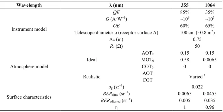
In our model, both the UV and NIR wavelengths were considered (i.e., 355 and 1064 nm). The corresponding instrumental parameters were chosen according to the existing spaceborne lidar systems. The most commonly used photo-detectors in UV and NIR are the photomultiplier tube (PMT) and the avalanche photodiode (APD), respectively. State of the art PMTs/APDs were considered for our simulations with their quantum efficiency (QE) and gain (G) shown in Table 1. The optical components (optical efficiency (OE), Table 1) used for these two wavelengths domains have similar properties. Other instrumental parameters (i.e., A, Rc, Δz) were considered as the same for both wavelengths in our
simulations (Table 1). 2.2.2. Atmospheric Model
The total optical thickness TOT(h), in the lidar equation sense as defined by Measures [44], is the sum of half the forest optical thickness (FOT) and the total atmospheric optical thickness (τ).
{ 𝑇𝑂𝑇(ℎ) =
𝐹𝑂𝑇(ℎ)
2 + 𝜏(ℎ)
Considering
𝑋(ℎ) = ∫ 𝛼ℎ𝑍𝑃 𝑋(𝑧) ∙ 𝑑𝑧, with 𝑋 = 𝐹𝑂𝑇, 𝑀𝑂𝑇, 𝐴𝑂𝑇, 𝑜𝑟 𝐶𝑂𝑇 (5)
where MOT is the molecule optical thickness, AOT is the aerosol optical thickness, and COT is the cloud optical thickness. αX is the extinction coefficient associated to each component X. FOT will be discussed
in Section 2.3.
Table 1. Instrumental, atmospheric and surface parameters chosen for the simulation.
Wavelength λ (nm) 355 1064
Instrument model
QE 85% 35%
G (A·W−1) ~106 ~103
OE 60% 65%
Telescope diameter ø (receptor surface A) 100 cm (~0.8 m2)
Δz (m) 0.75 Rc (Ω) 50 Atmosphere model Ideal AOT0 0.15 0.15 MOT0 0.58 0.0065 COT0 0 0
Realistic AOT Varied 1
COT Surface characteristics ρg (sr−1) 0.022 BERsimu (sr−1) 0.0065 0.0455 BERadjusted (sr−1) 0.005 0.035 η 1 0.96
1 Derived from MODIS observations.
Two atmospheric conditions are used in the model. Under the ideal atmospheric condition, there is no cloud (COT0 = 0), and typical medium values of AOT and MOT are considered (AOT0 and MOT0),
which are given in Table 1 for 2 wavelengths (355 and 1064 nm). However, realistic spaceborne observations are often performed in presence of clouds and aerosol plumes, which decreases the atmospheric transmission of laser beams. Hence, realistic atmospheric conditions are also used to improve the simulations. MODIS observations of COT and AOT are used in our model, which are considered to be representative. The AOTs are derived from the MODIS daily aerosol product MOD04 at the horizontal resolution of 10 km [46]. As AOTs are only given at 470, 550, and 660 nm, the Angstrom Exponent coefficients are used to estimate the AOTs at 355 and 1064 nm [47]. The COTs are derived from the MODIS daily cloud product MOD06 at the 1 km horizontal resolution [46], whereas the corresponding positions are derived from the MODIS geolocation product MOD03 [46].
2.2.3. Surface Characteristics
Surface reflectance (ρg) was calculated by Equation (2) using the ground echoes of many airborne
lidar sampling profiles. The values of ρg at 355 nm are found to be similar for all these measured profiles: ρg
= 0.022 ± 0.002 sr−1. Tang et al. [48] found out the surface reflectance at 1064 nm: ρg = 0.14 ± 0.03 sr−1. We
Backscatter to extinction ratio (BER) was calculated from the scattering phase function (P) inside
the canopy:
𝐵𝐸𝑅 = 1
4𝜋∙ 𝜔0∙ 𝑃𝜋 (6)
where ω0 is the single scattering albedo of scatters and Pπ is the backscatter scattering phase function.
There is little information about P, especially at the scale at a lidar footprint size of a few meters. As in Chen et al. [49], the Bidirectional Reflectance Distribution Functions (BRDF) from passive spaceborne measurements (multi-angular satellite POLDER data) was used to retrieve P using semi-empirical models, even though they are retrieved with pixels of several kilometers. More detailed BRDF modeling are given in Appendix B. Bendix et al. [50] show the variation of absorption and scattering with wavelength: there is strong absorption and little scattering in UV, whereas there is ~7 times more scattering in NIR. However, regarding the reflectance spectral dependency as documented in the same study, the behavior of the 490 nm (resp. 865 nm) channel seems very close to the one for the UV (resp. NIR) wavelength of 355 nm (resp. 1064 nm). The corresponding Pπ of the 490 nm (resp.
865 nm) channel can then be used for simulations at 355 nm (resp. 1064 nm). Both mean value and standard deviation of the retrieved Pπ are given in Table 2 for each considered forest type. They lead to
a BER close to 0.007 ± 0.002 sr−1 (resp. 0.046 ± 0.002 sr−1) in UV (resp. NIR). These BER values were
used in the following simulations and supposed constant in the canopy.
Table 2. Backscatter scattering phase function (Pπ) derived from the multi-angular satellite
POLDER data. The absorption coefficient is also given.
Period Pπ in “Mixed Forest” Pπ in “Evergreen Needle Leaf” Absorption Coefficient (1 − ω0) 490 nm 865 nm 490 nm 865 nm 355 nm 1064 nm January 1.79 ± 0.32 1.52 ± 0.15 1.62 ± 0.48 1.57 ± 0.15
~0.95 ~0.35 July 1.36 ± 0.42 1.36 ± 0.16 1.65 ± 0.44 1.53 ± 0.21
Multiple scattering coefficient (η), at different depths in the scattering layer, is deduced from the
ratio between the total lidar signal (including single scattering Ssingle and multiple scattering Smultiple) and
the number of single-backscattered photon as [29]:
𝜂(ℎ) = 1 −
ln (𝑆𝑠𝑖𝑛𝑔𝑙𝑒(ℎ) + 𝑆𝑆 𝑚𝑢𝑙𝑡𝑖𝑝𝑙𝑒(ℎ)
𝑠𝑖𝑛𝑔𝑙𝑒(ℎ) )
𝐹𝑂𝑇(ℎ) − 𝐹𝑂𝑇(ℎ𝑡)
(7) where ht is the top of the scattering layer.
The Multiple scattering (MS) effects in UV are negligible, and the typical value is η ~1. However the MS effects may become significant compared to the single scattering when switching from UV (355 nm) to NIR (1064 nm). Thus, for the Monte Carlo simulation, the MS coefficient (η) in NIR is derived as 0.96 ± 0.03 for different conditions (e.g., different space missions). The MS effects may impact the structural parameters retrieved from NIR lidar measurements and the associated uncertainties have to be assessed from the simulations.
Land-cover type is obtained with the MODIS product [46]. This parameter helps us choose the study
areas. Two MODIS land-cover type yearly products (chosen arbitrary for 2011) are used to identify the forest area: MCD12C1 (horizontal resolution of 0.05°) and MCD12Q1 (horizontal resolution of 500 m).
The classification scheme (“Land Cover Type 1”), defined by the International Geosphere Biosphere Programme (more information are available online [51]), is used in our simulations.
2.2.4. Platform Model
Airborne lidar. The main characteristics of the lidar system ULICE are given in Table 3. The laser
energy (E) is deliberately oversized (~7 mJ), which is compensated by optical densities (OD = 3) at the reception, in order to limit the parasitic signal related to the sky radiance. The vertical sampling resolution (Δz) along the lidar line-of-sight depends on the sampling frequency of the digitizer card and the laser pulse duration. The Centurion laser has a laser pulse duration between 6 and 7 ns, so the sampling frequency is chosen between 100 and 500 MHz leading to vertical sampling between 0.3 and 1.5 m. The vertical sampling of 0.75 m was the one most frequently chosen for the acquisition the lidar profiles used in the simulations. The pulse repetition frequency (PRF) is defined on the basis of the footprint sampling density needed in the forest sites and the aircraft speed, which ranges from 5 to 100 Hz for a full-waveform lidar system and was chosen to be 20 Hz during the field campaigns [42]. The energy distribution of laser beam is Gaussian according to the calibration in the laboratory. It can be considered as homogeneous for airborne measurements with small footprints (<5 m), but has to be taken into account for spaceborne measurements with lager footprints. The laser footprint size at the ground level is defined by the laser beam divergence and the platform altitude. Airborne lidar measurements were performed for flight altitude close to 350 m agl. According to the divergence of the laser, it leads to footprints between 2 and 5 m in diameter over the temperate forests, and ~10 m in diameter for tropical forests. These profiles can be further recombined to simulate profiles in a compatible footprint of a spaceborne lidar.
Spaceborne lidar systems. Lidar systems have been already embedded onboard the satellites. Even
though none of their purposes is to detect and sample forests, some instrumental parameters and the orbits of the main spaceborne lidar missions can be considered as the references for our simulations. Four missions were chosen and will be considered: the Geoscience Laser Altimeter System (GLAS) onboard the past mission ICESat (Ice, Cloud, and land Elevation Satellite) to detect ice-elevation changes in Antarctica and Greenland [52]; the future Climate Mission MERLIN (Methane Remote Sensing Lidar Mission) with the payload of a Methane Integrated Path Differential Absorption (IPDA) LIDAR emitting at 1645 nm, dedicated to the measurements of the greenhouse gas Methane [53]; the near-future ADM-Aeolus (Atmospheric Dynamics Mission Aeolus) mission carrying the Atmospheric Laser Doppler Instrument (ALADIN) for global wind profile observations [54]; the current CALIPSO (Cloud-Aerosol Lidar and Infrared Pathfinder Satellite Observations) mission carrying the Cloud-Aerosol LIdar with Orthogonal Polarization (CALIOP) to improve the understanding of the role of aerosols and clouds in the Earth’s climate system [55]. The International Space Station (ISS) is also considered as a potential platform for a future spaceborne canopy lidar system, an example of recent mission CATS (Cloud-Aerosol Transport System) for the atmospheric purpose is given at [56].
Actual parameters of these referenced spaceborne lidar missions were found out through research papers [53,57–60], and are given in Table 3. As they were not designed for forest studies, the sampling vertical resolution (Δz) for CALIPSO, MERLIN, and ADM-Aeolus missions is too large. Their parameters
are then modified for a 0.75 m resolution as the one of our airborne lidar ULICE. The Δz of the ICESat mission keeps its own value since one of its targets is the surface study.
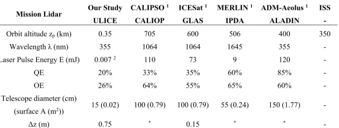
Table 3. Actual parameters for ULICE and referenced spaceborne lidar missions.
Mission Lidar Our Study ULICE CALIPSO 1 CALIOP ICESat 1 GLAS MERLIN 1 IPDA ADM-Aeolus 1 ALADIN ISS - Orbit altitude zp (km) 0.35 705 600 506 400 350 Wavelength λ (nm) 355 1064 1064 1645 355 - Laser Pulse Energy E (mJ) 0.007 2 110 73 9 120 -
QE 20% 33% 35% 60% 85% -
OE 26% 64% 55% 65% 60% -
Telescope diameter (cm)
(surface A (m2)) 15 (0.02) 100 (0.79) 100 (0.79) 55 (0.24) 150 (1.77) -
Δz (m) 0.75 * 0.15 * * -
* the actual Δz cannot be used for forest sampling, and chosen to be 0.75 m; 1 These parameters of spaceborne
lidar missions were found out through research papers [53,57–60]; 2 Calculated by E0/100D with emitted laser energy E0 = 7 mJ and optical densities OD = 3.
2.3. Inverse Model
In order to retrieve forest vertical structures, it is necessary to detect the intensity peaks of both the canopy and ground echoes in the full-waveform lidar signals. The TTH is calculated as the distance between the first return at the upper surface of the vegetation and the last return from the ground surface. Following the signal processing described in Shang and Chazette [42], the ground echo was first detected compared to the noise level, which can be inferred from the signal remaining after the ground echo when only the instrumental noise exists. The canopy echo was then detected, considering the atmospheric signal just above the trees.
To simplify the calculation, the range-corrected lidar signal is introduced, which is defined as the product of the backscattered lidar signal Sv(h) and the square of the distance between the laser emission
and the target. The integrated canopy signal Rv(h) is defined as the integral of the range-corrected lidar
signal from the canopy top TTH to height level h. As BER is assumed to be constant for all canopy levels (i.e., BER0) and η ~1 in UV, Rv(h) can be expressed, after correction of the atmospheric transmission, as:
{𝑅𝑣(ℎ) = ∫ 𝑆𝑣(𝑧) ∙ (𝑍𝑝− (ℎ + 𝑧𝑔𝑟𝑜𝑢𝑛𝑑))2∙ 𝑑𝑧 𝑇𝑇𝐻
ℎ
𝑅𝑣(ℎ) = 𝐾0∙ 𝐸0 ∙ 𝐵𝐸𝑅0∙ [1 − 𝑒𝑥𝑝(−𝐹𝑂𝑇(ℎ))]
(8) The FOT can then be derived as:
𝐹𝑂𝑇(ℎ) = − 𝑙𝑛 (1 − 1
𝐾0∙ 𝐸0∙ 𝐵𝐸𝑅0∙ 𝑅𝑣(ℎ)) (9)
The FOT, defined as the optical thickness in a forest layer between the considered height h and the canopy top TTH, depends on the canopy extinction coefficient αFOT, which is then derived from
𝛼(ℎ) =∂ln [1 −
1
𝐾0∙ 𝐸0∙ 𝐵𝐸𝑅0∙ 𝑅𝑣(ℎ)]
∂ℎ (10)
This solution is consistent with the one derived from the statistic consideration made by
Lefsky et al. [15]. Canopy extinction coefficient is a fundamental parameter used in our direct model to simulate the lidar signal by using the lidar equation under the hypothesis of “single scattering”.
The QMCH (quadratic mean canopy height) parameter, which can be used to evaluate the aboveground biomass [42], is also a function of the extinction coefficient [15]:
𝑄𝑀𝐶𝐻 = √∫ 𝛼(ℎ) ∙ ℎ0 2∙ 𝑑ℎ 𝑇𝑇𝐻
(11) 2.4. Sampling Sites
Several forest sites have been sampled between 2008 and 2014 to build significant sample sets of different ecosystems, from temperate to tropical forests (Table 4). Our first airborne lidar measurement was conducted over the Landes forest, located in the southwest of France (44°N, 1°W) and mainly composed of maritime pines. The second experiments were carried out, during both winter and summer season, above the Fontainebleau forest in the southeast of Paris (48°N, 2°E), which is a temperate deciduous forest composed of evergreen and broadleaf trees. Forests of white oaks and a plantation of poplars in and close to the OHP (Observatoire de Haute-Provence, 44°N, 6°E) were also sampled during spring 2012. Recently, airborne lidar measurements were conducted in May 2014 over several tropical forest sites of Réunion Island (21°S, 55°E), including rain and montane cloud forests.
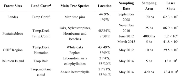
Table 4. Description of the sites sampled with the airborne lidar ULICE between 2008 and 2014.
Forest Sites Land Cover1 Main Tree Species Location Sampling
Date
Sampling Area
Laser Shots Landes Temp.Conif. Maritime pins 44°9ʹN,
1°9ʹW
September
2008 170 ha 62.3 × 10³ Fontainebleau Temp.Deci.
Temp.Conif.
Oaks, Sylvester pines, Hornbeams and Beeches 48°24ʹN, 2°38ʹE November 2010 25 ha 86.9 × 10³ June 2012 4000 ha 1.2 × 10⁶ March 2013 5 ha 41.8 × 10³
OHP2 Region Temp.Deci.
Plantation
White oaks Poplars
43°49ʹN,
5°49ʹE May 2012 10 ha 29.5 × 10³ Réunion Island Trop.Rain Labourdonnaisia
calophylloides
21°4ʹS,
55°30ʹE May 2014 5 ha 12 × 103 Trop.montane
cloud Acacia heterophylla
21°21ʹS,
55°44ʹE May 2014 420 ha 48.4 ×10³
1 Temp.: temperate, Conif.: conifer, Deci.: Deciduous, Trop.: tropical; 2 OHP: Observatoire de Haute Provence.
The tree species included in the sampled sites of temperate forests constitute about 70% of the ones encountered in the western European forests (distribution maps of tree species are available from the European Forest Genetic Resources Programme website: [61]). Temperate forests significantly impact the atmospheric chemistry and mainly the ozone concentration in the troposphere, especially at regional
scales [2]. Although composed of small trees, the rainforests of the Réunion Island are representative of many tropical forest areas in terms of density [62]. For the boreal forests, the lidar budget is easier to be built because they are less dense. If the lidar-derived information is reliable for the low-/mid-latitude (tropical/temperate) forests, it will also be reliable for the higher latitudes.
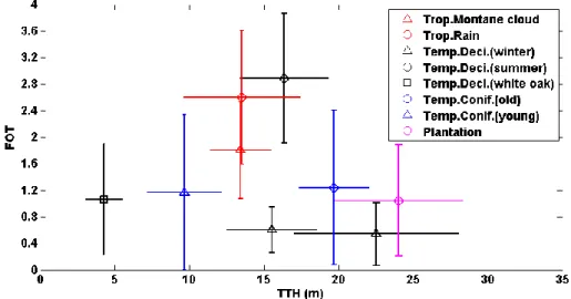
Nine plots of ~5 ha were studied, representing different biomes. (1) 3 plots in Fontainebleau forest: a forest plot of oaks and hornbeams sampled in winter 2010, a wild broadleaf forest plot sampled in summer 2012, and a plot of the same location sampled in winter 2013, which represent temperate deciduous trees in two typical seasons; (2) 1 plot of white oaks in OHP Region, representing temperate deciduous trees in spring; (3) 2 plots in Landes forest in September 2008, for different mature (~50 and ~10 years, respectively) maritime pines, representing temperate conifer trees, which do not change much with the seasons; (4) 2 plots of tropical forests on Réunion Island in May 2014, one for tropical lowland rainforest, and the other for tropical montane cloud forests; (5) 1 plot of plantation of poplars in OHP Region in June 2012. The FOT and TTH of every lidar profiles in each plot were calculated through the inverse model; their mean and standard deviation values are shown in Figure 3. The temperate deciduous forests have a small FOT in winter but a big FOT in summer, because of tree crowns with dense leaf amounts. The FOTs of temperate conifer forests of different ages (different TTHs) are similar. The tropical forests are dense and have a big FOT as expected. However, the results show that the wild temperate broadleaf forests in summer can be denser than the studied tropical forests. These distributions of FOTs and TTHs will be considered in our simulator.
Figure 3. Mean (marker) and standard deviations (line segments) of lidar-derived forest
optical thickness (FOT) and tree top height (TTH) for 9 forest plots. Trop.: tropical, Temp.: temperate, Deci.: Deciduous, Conif.: conifer.
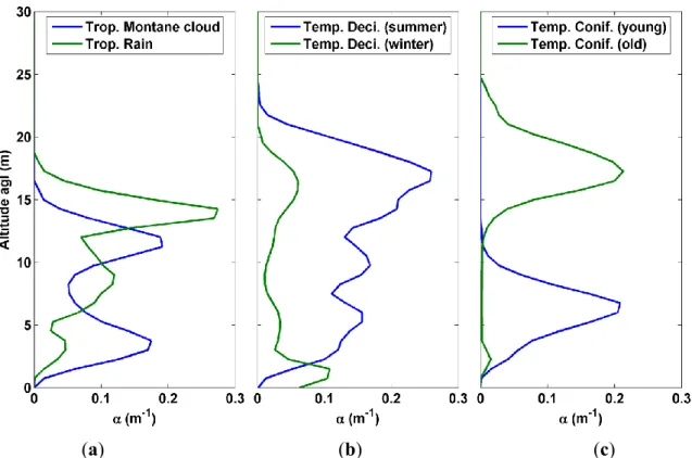
In the previous plots, several representative profiles were selected as the input of the EES for the numerical simulations. The vertical profiles of the extinction coefficient of sampling profiles were calculated through the inverse model; six of them are shown in Figure 4 as examples. The extinction coefficient not only significantly varies from one site to another, but also varies within each sampled site. The selected sample profiles are located at the center of the distribution in terms of both α and FOT in the sampled site.
(a) (b) (c)
Figure 4. Examples of extinction coefficient profiles of 6 selected lidar profiles: (a) tropical
montane cloud and rain forest; (b) temperate deciduous forest in both summer and winter, and (c) temperate conifer forest with young (10 years old) and old trees (50 years old).
The tropical montane forest represents an approximate average of the measured biomes (Figure 3). A detailed distribution of the FOT is given in Figure 5 for this case, which will be considered as the reference in the following.
Figure 5. Blue bars: Forest optical thickness (FOT) distribution in tropical montane cloud
forest (Table 4). Black curve: cumulative probability density functions (CPDF)/Cumulative distribution function F of FOT.
2.5. Adjustment of Parameters: Relevance of the Direct Model
For a given vertical profile of the extinction coefficient (α), simulated lidar profile can be calculated by using the direct model (Section 2.2). However, before these simulations, it is necessary to adjust two important parameters involved in the lidar equation: the instrumental constant K(λ), and the backscatter to extinction coefficient BER in the canopy. They have been adjusted by comparing the simulation with the measurements for each forest site.
K(λ) needs to be adjusted because of uncertainties on several optical components of the lidar (e.g., transmittance of optical lenses, laser energy, detector gain). The molecular extinction and backscatter coefficients are determined based on the polynomial approximation proposed by Nicolet [63] as in Chazette et al. [64]. The aerosol contribution has been assessed during the ascent of the ULA as in Chazette et al. [41]. Note that for all the sites, the aerosol optical thickness between the ground and the ULA was less than 0.03. Hence, we found a relative correction within 5% on K(λ).
The BER in the canopy previously retrieved was used for the sampling cases. Nevertheless, the simulated profiles did not exactly match the measurements by ~30%, because of the hypotheses used in our simulations. Therefore the BER in UV was adjusted to 0.005 ± 0.002 sr−1 by comparing measured
and simulated canopy signals via the EES. Such a value is very close to the initial value and it is in the error tolerance (~30%) for a simulator.
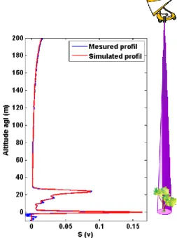
Taking into account these adjustments, the lidar profile can be well simulated as an example given in Figure 6. The ground-echo is well reproduced, as well as the response of the forest below 28 m agl. The simulated lidar signal in the atmosphere, i.e., above ~28 m agl, also matches very well with the measurements. The direct model is thus found relevant for realistic simulations from airborne and spaceborne platforms.
Figure 6. Simulated lidar signal (Red) superposed on measured lidar signal (Blue) as an
3. End-to-End Modeling
In this section, the retrievals of structural and optical parameters from the simulations of an airborne/spaceborne lidar system working at both wavelengths of 355 nm and 1064 nm are studied through the end-to-end simulator (EES). We assess the optimal laser footprint size and signal-to-noise ratio (SNR). Both the surface slope and the multiple scattering effects on the lidar signal are computed and discussed.
3.1. Laser Footprint Size
For a given PRF, the small-footprint of the laser beam at the ground level brings more details and accuracy to assess forest vertical structures; whereas the large-footprint increases the probability of ground echo detections by increasing the laser penetration ability. The latter is more suitable for spaceborne lidar observations.
In our airborne measurements performed at 355 nm, a small-footprint size (~2 m in diameter at the ground level) was used for temperate forests. With this footprint size the laser penetration is good enough to detect forest vertical parameters for deciduous forests in winter and conifer forests. The probability density functions (PDF) of GE detections (PDFGE) for lidar profiles was found to be ~1 for these cases.
However, PDFGE in summer for temperate deciduous forests was found to be ~0.2. This was due to the
signal attenuation by canopy leaf strata and the effects of the ground cover vegetation. We performed the lidar measurements by increasing the footprint size to be ~4 m in diameter for the same site, leading to a PDFGE ~0.4. The footprint size was increased to be ~10 m for tropical forests, which improved the
capacity of the laser penetration in the canopy. As it was found that 10 m is not enough for ground echo detections (70% probability) through dense forests (FOT > 3), the footprint diameter has to be set to a larger value, which will be a compromise between the probability to detect the ground, the horizontal sampling density of lidar footprints, and the SNR.
To simulate large laser footprints, lidar profiles measured with a small footprint size (e.g., 2 m) were combined to get a simulated lidar profile with a larger footprint size (as schematized in Figure 7), taking into account the Gaussian energy distribution of the laser beam.
Figure 7. Illustration of the combination of lidar profiles to simulate a lidar signal of a larger
footprint. R is the radius of the simulated larger footprint, ri is distance between ith laser shot
The sample case of temperate deciduous forests in summer was chosen, since the corresponding FOT is the biggest one. By entering different footprint sizes into our model, corresponding PDFGE was
calculated through simulated lidar profiles. A relationship between PDFGE and the footprint diameter was
found as shown in Figure 8, which indicates an optimal laser footprint diameter of ~20 m for the oak forest in summer (FOT ≈ 3). This optimal footprint of 20 m diameter will be considered in the following.
Figure 8. The probability density functions (PDF) of the good detection of the ground echo
(GE) vs. footprint diameters.
3.2. Optimal SNR and Related Uncertainties
The optimal SNR is defined as the minimal one to get a good detection of forest parameters. The SNR at the ground level (GE SNR) is chosen as an indicator for the evaluation. Of course, a better detection can be obtained for a greater SNR, but the lidar characteristics are strongly constrained for air- and space-borne systems by this parameter. Getting a lower SNR, there will be less constraint on the payload (e.g., energy, mass, volume).
Optimal SNR for GE detection. The input signals are simulated from airborne measurements
considering a 20 m footprint. By applying the EES, the PDF of the ground echo (GE) detection vs. the GE SNR is derived (Figure 9). The result shows that the optimal SNR at the ground level to get a good GE detection is ~6.
Optimal SNR for forest parameters. The GE detection is not sufficient to ensure a good assessment
of both forest vertical structures and optical parameters. Therefore, the optimal SNR is studied by considering the uncertainties on these parameters. The acceptable uncertainty on the lidar-derived TTH (ɛTTH) and QMCH (ɛQMCH) is 1.5 m and 5%, respectively, as described in Shang and Chazette [42]. The
uncertainty on α depends on the one on FOT. Hence, the FOT at the canopy bottom, which is an integrated value, was preferred for this study instead of α. Figure 10 gives the results of the relative error simulations to retrieve the TTH, QMCH and FOT for different GE SNR. We can consider that sufficient accuracy can be obtained for all parameters for a GE SNR larger than 10. In the following, the link budget of the spaceborne lidar was then assessed using the optimal SNR0 = 10.
Figure 9. The probability density functions (PDF) of the good detection of the ground echo
(GE) vs. SNR at the ground level (GE SNR). The optimal SNR of 6 is highlighted by the black vertical dotted line.
Figure 10. Uncertainties 1 on TTH, QMCH and FOT for different GE SNR. 1 Mean values
for all sampling sites. 3.3. Lidar Signal Distortion 3.3.1. Surface Slope
As highlighted by Yang et al. [65] and Hancock et al. [66], surface slope has an effect on the lidar accuracy for large footprint lidar systems. This lidar signal distortion due to the surface slope may be no longer negligible when considering a footprint of 20 m in diameter. It affects both the canopy and the ground echoes and may modify their locations in a lidar profile and the SNR level. In this way, it impacts the link budget of the lidar system. Simulations were operated over a simulated homogenous forest
containing identical trees (see the illustration of Figure 11a). On the one hand, different ground slopes (0°, 15°, 30° and 45°) were applied for a combined lidar signal in a 20 m footprint. Results (Figure 11b) show that the lidar profile is strongly affected by slopes larger than 30°. On the other hand, different footprint sizes (5m, 20m and 40 m) were used for a ground slope of 30° (Figure 11c). As expected and shown in Figure 11, the lidar signal decreases and the distortion increases when the slope or the footprint size increases. This leads to a dispersion of the ground echo on a larger altitude range and to a loss of precision when retrieving the structural parameters. For instance, a slope of 30° and a footprint of 20 m in diameter lead to a relative uncertainty of 10%–30% on TTH, QMCH and FOT. This means the surface slope effect has to be considered in the link budget of spaceborne lidar observations; which is equivalent to a decrease of ~50% of the GE SNR and then leads to significant increase of the necessary lidar payload (e.g., emitted energy, telescope diameter).
(a) (b) (c)
Figure 11. (a) Illustration of the simulation of a forest site with a slope θ; (b) Example of
different lidar signal simulated through the canopy of Fontainebleau for different slopes between 0 and 45° for a footprint of 20 m; (c) Example of different lidar signal simulated for different footprint sizes with slope of 30°.
3.3.2. Multiple Scattering Effects
The multiple scattering (MS) contributions are taken into account through the MS coefficient η [29], and depend on the wavelengths [66]. As previously explained (Section 2.2.3), this effect is negligible in UV (355 nm, η ≈ 1), but not in NIR (1064 nm, η ≈ 0.96). An example of simulations in UV is given in Figure 12a; there is no much difference between the single scattering signal (green curve) and the total simulated signal (single and multiple scattering, cyan curve). Simulations in NIR for the same conditions are given in Figure 12b; the multiple scattering contributions (red curve) significantly affect the lidar signal. By comparing the single scattering signal and the total simulated signal, bias of ~2–3 m can be observed on the location of the tree crown and relative errors of ~5% were found on the QMCH and FOT estimations. This result also confirms the study of Kotchenova et al. [67], who highlighted that multiply scattered photons magnify the amplitude of the reflected signal, especially that originating from the lower portions of the canopy. Similar uncertainty may affect the location of the ground echo if there is undergrowth. Such bias can be partially corrected after the retrieval of the vertical profile of the extinction coefficient and will be ignored hereafter. Note that the multiple scattering effects can be corrected at the first order considering the FOT. It will not be taken into account hereafter.
(a)
(b)
Figure 12. Multiple scattering effect simulations at (a) 355 nm and (b) 1064 nm for oaks in
summer by using a similar orbit of ISS at 350 km.
4. Link Budget
In this section, the link budget of spaceborne lidar systems will be discussed. We defined realistic orbits based on past and current satellites (see Table 3). Two typical areas were chosen for boreal and tropical forests, which are the main carbon reservoirs. The sites were analyzed during the seasons where the probability of having a significant cloud cover is minimal. In our link budget, we took into account the decrease of the SNR due to the aerosol and cloud optical thicknesses which are derived from operational satellite measurements (MODIS) chosen arbitrary for 2011. The different working hypothesis and the corresponding results are presented in this section.
4.1. Link Budget under Ideal Atmospheric Conditions
The link budget is firstly studied under ideal atmospheric conditions (Atmosphere model in Table 1). In our simulation, only shot noise is taken into account as the others noise sources can be considered negligible (see Appendix A). The SNR of lidar signals depends on the instrumental parameters, the
atmospheric optical thickness, the surface characteristics and the platform altitude. For a given lidar system, the SNR decreases exponentially as the FOT increases.
Firstly, we considered the actual instrumental parameters of the four referenced spaceborne lidar missions (CALIPSO, ICESat, MERLIN, and ADM-Aeolus) as shown in Table 3. Here we considered two types of forest with FOT of 1 or 2. The corresponding GE SNR of these spaceborne lidar systems are calculated, and given in Table 5. Lidar products of the ICESat mission have been used for forest studies (e.g., [48,68–70]). Through the results of our EES, the GLAS lidar can well mapping the open forest with a FOT ≤ 1, which occupies ~30% of the forest area by considering the FOT distributions derived from our airborne lidar measurements. But it cannot well study denser forests with a lager FOT due to a low SNR.
Table 5. SNR at the ground level (GE SNR) of lidar signal by using actual parameters of
four spaceborne lidar missions (Table 3), and the Atmosphere model and Surface characteristics in Table 1.
Mission CALIPSO ICESat MERLIN ADM-Aeolus
Lidar CALIOP GLAS IPDA ALADIN
Orbit altitude zp (km) 705 600 506 400
GE SNR FOT = 1 24.5 10.0 9.1 12.9
FOT = 2 14.8 6.1 5.5 7.9
Secondly, our EES simulations were performed for lidar systems with same instrumental parameters (given in Table 1) onboard five spatial platforms: CALIPSO, ICESat, MERLIN, ADM-Aeolus, and ISS. The values of required energies (E) were found out at both the UV and NIR wavelengths (Table 6), by considering getting SNR ~10 at the ground level.
These simulations show that it will be difficult to detect dense forests (FOT > 2) at a UV wavelength. Even for the ISS, the required energy of the lidar system is ~220 mJ to detect a medium dense forest (FOT = 2), which means good detections for temperate deciduous forests in winter and temperate conifer forests, but poor detections for temperate deciduous forests in summer or tropical forests. The values of E retrieved in the NIR domain are more realistic for a spaceborne mission because they remain lower than 80 mJ for medium dense forests (FOT ≤ 3), which represent ~90% surface of the forest area according to the referenced FOT distribution (Figure 5). Thus, only the NIR domain will be considered hereafter for the link budget for realistic atmospheric conditions. Obviously, the low orbit will be preferred for dense forests (FOT > 2).
Accounting for the above considerations, for a given lidar system and a chosen orbit, there is a maximum value of the total optical thickness (TOTmax) for which the ground echo is still detectable. The
lower the orbit is, the larger TOTmax will be, as expressed by Equation (1). If we take an example of a
lidar system with instrumental parameters given in Table 1, emitting 100 mJ laser pulses at 1064 nm, the TOTmax for systems onboard five spaceborne platforms were calculated and given in Table 6.
As in Equation (4), the TOT is the sum of half the FOT and the total atmospheric optical thickness τ, the latter one is equal to 0.1565 under ideal atmospheric conditions (Table 1). Then, we can get the corresponding FOTmax (maximal forest optical thickness) to study the forest density limit of each spaceborne
Table 6. Required energy E in 355 nm or 1064 nm to get a good detection (GE SNR ~10)
under ideal atmospheric conditions for 4 forest classes. Each class represents forests with forest optical thicknesses (FOT) less than a certain value (1, 2, 3, 4). The corresponding area proportion of each forest class among the total forest area is also given. An example of maximum value of the total optical thickness (TOTmax) at which the detection is still good,
for a lidar system emitting 100 mJ at 1064 nm, is also given. The instrumental parameters used are given in Table 1.
Orbit CALIPSO ICESat MERLIN ADM-Aeolus ISS Orbit altitude zp (km) 705 600 506 400 350 Required laser pulse energy Forest class Forest area proportion E (mJ) at 355 nm FOT ≤ 1 30% 333.6 241.7 171.9 107.4 82.2 FOT ≤ 2 75% 906.9 656.9 467.2 292 223.5 E (mJ) at 1064 nm FOT ≤ 1 30% 11.4 8.3 5.9 3.7 2.8 FOT ≤ 2 75% 31.0 22.5 16.0 10.0 7.7 FOT ≤ 3 92% 84.4 61.1 43.5 27.2 20.8 FOT ≤ 4 98% 229.4 166.1 118.2 73.8 56.5
Example: laser pulse energy E = 100 mJ at the wavelength of 1064 nm
TOTmax for good detection
(TOT = FOT/2 + τ, Equation (4)) 1.74 1.90 2.07 2.31 2.44
FOT: forest optical thickness. TOT: total optical thickness. τ: total atmospheric optical thickness.
4.2. Link Budget under Realistic Atmospheric Conditions
Spaceborne observations are always performed in presence of clouds and aerosol plumes, which increase the total atmospheric optical thickness τ and decrease the SNR. In this section the effect of cloud and aerosol covers are taken into account to complete the previous link budget performed under ideal atmospheric conditions. We first present the assumptions of the study and finish by the results and discussions.
4.2.1. Study Areas
The link budget is performed on the most important forest types. The tropical and boreal forests are the broadest ones with surface of ~2000 × 106 (10% of land) and ~1000 × 106 ha, respectively (by the
Office National des Forêts, [71]). From the global land-cover map in 2011 derived from MODIS product MCD12C1 as shown by Figure 13a, we chose two areas of 10 × 6 (shown by the black boxes in Figure 13a): one is located in Congo basin (Africa) (1°N, 20°E) which represents the tropical forest with the dominant land-cover of evergreen broadleaf forests; the other is located in North-Asia (58°N, 101°E), close to the lake Baïkal in Russia, which represents boreal forests with mainly mixed forests and a few needleleaf forests. The more accurate land-cover maps derived from MCD12Q1 (MODIS) for the two selected areas (shown in Figure 13b) were used in our model.
(a)
(b)
Figure 13. (a) Simulated orbits of ISS (in pink) and ICESat (in blue) of 1 day over the
simplified land-cover map derived from MCD12C1 (MODIS) of 2011 with a spatial resolution of 0.05°; (b) Simulated orbits of 26 days over the Congo basin (Africa) zone (left) and lake Baïkal (Asia) zone (right), land-cover maps were derived from MCD12Q1 (MODIS) of 2011 with a spatial resolution of 500 m. The different green colors indicate five dominant forest types as named in (a).
4.2.2. Study Periods
For each area, we selected one month for the simulation. The ideal period is when there are fewer clouds and smaller AOT. The European Center for Medium-Range Weather Forecasts (ECMWF) model gives the probability of high, middle, low and total cloud cover at the global scale, at a spatial horizontal resolution of 0.75° and a temporal resolution of 6 hours [72]. The mean values and standard deviations of the probabilities of cloud presence over the considered areas of each month of 2011 are studied. The monthly AOT is derived by using the MODIS Atmosphere Monthly Global Product MOD08_M3 at the horizontal resolution of 1° [46], which is also considered for the two areas. There is no AOT value for the North-Asian site during the winter due to excessive cloud cover. We thus chose December and June for the Congo basin and Lake Baïkal areas, respectively, when the average monthly probability of cloud is the lowest in order to promote the cloud free condition.
4.2.3. Orbit Simulation
The existing orbits were considered to perform orbit simulations. The ISS is the first candidate, since there are most resources (e.g., enough energy supply) available onboard. The second one is the ICESat, because the onboard GLAS lidar was already used for some forest studies [68–70,73–75]. The SPOT (Satellite for observation of Earth) could be another candidate, but its altitude (832 km) is too high for lidar measurements. Thus, the two existing orbits of ISS and ICESat were chosen for the simulation by using their respective orbital characteristics, because they are more realistic for the proposed mission. Note that the inclination of the ISS orbit does not permit measurements in the higher latitudes.
The revisit cycle of both orbits was chosen to be 26 days, as for the SPOT mission, which is dedicated to surface survey. The simulated orbits are shown in Figure 13, with 1 day’s revolutions for the global area and 26 days’ revolutions for the 2 selected areas.
4.2.4. Atmospheric Distributions
The sampling frequency of the onboard lidar is chosen to be 10 Hz by taking into account the spatial horizontal resolutions of the considered satellite data (no significant statistical differences are observed for higher PRF). For each lidar shot, the corresponding AOT and COT were derived from the nearest (in space and time) MODIS data. For one revisit cycle, we calculated the distribution (histogram) and then the cumulative distribution function F(τ) of the total atmospheric optical thickness τ for the lidar shots inside the two selected areas (Figure 14).
Total number of lidar shots: 23898 Shots with valid MODIS data: 15512
Total number of lidar shots: 18539 Shots with valid MODIS data: 12596
(a) (b)
Total number of lidar shots: 18880 Shots with valid MODIS data: 9458
(c)
Figure 14. Blue bars: distribution1 of total atmospheric optical thickness τ at 1064 nm for
one revisit cycle (26 days) of the satellite over the two selected areas: Congo basin (Africa, tropical forest) and Lake Baïkal (Russia, boreal forest) with 2 satellite orbits (ISS and ICESat). Black curve: cumulative probability density functions (CPDF) of τ. The number of the lidar shots following ISS/ICESat orbit inside each selected area is given, as well as the corresponding valid value number of τ given by MODIS. 1 The distribution is truncated at 4.
(a) ISS—Congo basin area; (b) ICESat—Congo basin area; (c) ICESat—Lake Baïkal area. 4.2.5. Discussion on Probability of Good Detections for One Satellite Pass
As mentioned before, for a given lidar system and a chosen orbit, there is a TOTmax below which the
detections are always good (SNRGE ≥ 10). The atmospheric and the forest optical thicknesses are then
complementary. A value of FOT is associated with each single lidar profile; if FOT ≤ 2TOTmax the
probability of good detections depends on the probability distribution of τ, F(τ). This probability can be computed by:
p = F (TOTmax − 𝐹𝑂𝑇
2 ) (12)
For example, TOTmax has been found as equal to 2.44 when considering an emitted energy ~100 mJ
for a NIR lidar payload embedded onboard the ISS. If we want to detect forest with FOT ≤ 3, which correspond to 92% of the forest from our FOT distribution reference, this probability is p = F (τ = 0.94) ~0.73 (see the gray dash line in Figure 14a). With the same lidar onboard ICESat, we found TOTmax = 1.90 and
then p = 0.62 and 0.59 for tropical and boreal forests, respectively. These TOTmax values are reported in
Table 6 for each relevant spaceborne mission. 4.2.6. Number of Satellite Revisits
Until now the link budget accounted for the forest detection using only one lidar profile (i.e., one satellite revisit). The number of satellite revisits can be increased to improve the probability of good detection. Considering the forest to be stationary, for k passes of the satellite over the same forest pixel, the probability (P) of having at least one good detection is given by:
P = 1 − (1 − p)k (13)
Obviously, the number of required revisits k changes with FOT values. Taking the previous examples of observations of tropical forest site with FOT = 3, if we want a probability of good detection P ≥ 0.99 (an arbitrary choice), we need k = 4 or 5 when considering a lidar system onboard the ISS or ICESat, respectively.
This number of revisits is important because it will strongly influence the spatio-temporal resolution of the lidar sampling from a spaceborne platform. There is a compromise to find between the revisit cycle and the sampled forest area. An increase of k induces a larger distance between satellite ground tracks, unless considering longer integration periods, exceeding a month. For a tropical forest that is not to change much during the year, we can consider a sample with a number of revisits spread over one year. The distance between the ground-tracks will be reduced (~50 km). For forests that change with the season, it will be better not to exceed one month and thus to increase the distance between the ground tracks. Hence, there is a trade-off between the temporal resolution, spatial resolution and payload (telescope size, energy). The solution also depends on the technical capabilities.
5. Discussion and Conclusions
Airborne lidar measurements were performed over several temperate and tropical forests sites, which allowed for building a representative database of lidar vertical profiles. From these lidar measurements, a semi-empirical approach was applied using the radiative transfer equation applied to the laser beam propagation into a scattering medium. An end-to-end simulator was developed to simulate and analyze the performance of both air- and space-borne lidar systems. The uncertainties on structural and optical parameters (tree top height, quadratic mean canopy height, and extinction coefficient) for spaceborne observations were estimated. The surface slope and the multiple scattering effects on the lidar signal were discussed, and proved to be not negligible for spaceborne observations leading to a relative error ~10%–30% on the retrieved parameters. The optimal signal-to-noise ratio was discussed for both ultraviolet (UV) and near infrared (NIR) wavelengths. The link budget for several platforms was built up for the two selected wavelengths (355 and 1064 nm), first under ideal atmospheric conditions (i.e., no cloud and medium aerosol content: aerosol optical thickness of 0.15), and then considering more realistic atmospheric scattering properties.
We confirm that the UV wavelength is suitable for airborne lidar measurements. However, UV lidar is not a good candidate for spaceborne missions due to low atmospheric transmission and strong absorption by the vegetation in the UV domain. The required energy in UV is ~30 times larger than in NIR through our simulations. It may be possible to use a UV lidar with ~80 mJ energy onboard the ISS platform, but only for forests with an optical thickness less than 1, corresponding to temperate deciduous forests in winter or temperate conifer forests. Hence, a wavelength in the NIR is preferred for a spaceborne lidar system dedicated to forest survey at the global scale, as medium dense forests (e.g., FOT ~2) can be well detected for all considered orbits from the ISS to the CALIPSO missions. But for the denser forests (e.g., temperate deciduous forests in summer or tropical forest with FOT > 2), a lower orbit is preferred and the number of satellite revisits should be increased to reach a good detection probability.
Spaceborne lidar dedicated to canopy can also be used for atmospheric studies because the emitted energy needed for forest study is comparable to the one of missions as CALIPSO. It can be a continuation
of the CALIPSO/CALIOP or further the ADM-Aeolus/ALADIN or EARTHCARE [76] missions. A specific spaceborne canopy lidar mission has been considered as a priority in the medium term by the French space agency following its prospective seminary held at La Rochelle in 2014.
Acknowledgment
The experiments have been funded by the Centre National d’Etudes Spatiales (CNES, English: National Centre for Space Studies) and the Commissariat à l’Energie Atomique et aux Energies Alternatives (CEA, English: French Alternative Energies and Atomic Energy Commission). The authors also thank the support offered by the Direction Générale de l’Armement (DGA, English: General Directorate for Armament). The POLDER/PARASOL BRDFs databases, offered by CNES, have been elaborated by the LSCE, and provided by the POSTEL Service Center. The authors are grateful to Fabien Marnas and Julien Totems for their help during the lidar experiments. The authors also thank Nicolas Baghdadi, Patrick Rairoux, Shushi Peng and Julien Totems for reviewing this paper.
Author Contributions
Both authors contributed extensively to the work presented in this paper.
Appendix A: Sources of Noise
For an instrumental link budget the contribution of each noise source has to be considered. There are five different and independent kinds of noise: the background-radiation noise, the shot noise (σS), the
dark-current noise (σD), the Johnson-Nyquist noise (σJN), and the quantification noise (σQ). Their
standard deviations are expressed by the symbol σ.
The background-radiation noise is negligible in our airborne measurements, because a strong optical density (OD ~3) was used to compensate the large field-of-view (~4 mrad). It is also negligible in our simulated spaceborne measurements with a much smaller field-of-view(<57 µrad). We take an example of a NIR (1064 nm) lidar system onboard the ISS with instrument parameters shown in Table 1, and an interference filter of 0.45 nm bandwidth [60]. Via the 6S radiative transfer modeling [77] for the worst case (i.e., solar and satellite zenith angles are both 0°), the background sky radiance was found to be 0.2 W·m−2·sr−1·nm-1. The background light is then evaluated [44] as 1.8 × 10⁻⁷ A, which is negligible
compared to the lidar signal.
In analog detection mode, lidar signal S is expressed in volt with Rc the load resistance. Since the
noise was expressed as a current, the signal-to-noise ratio (SNR) can be expressed as follows [44]:
𝑆𝑁𝑅 = 𝑆/𝑅𝑐
√𝜎𝑆2+ 𝜎𝐷2+ 𝜎𝐽𝑁2+ 𝜎𝑄2 (A.1)
{ 𝜎𝑆(𝜆, ℎ) = √ 𝐺 ∙ ħ𝑐𝜆 ∙ 𝜁 ∙ 𝑐 2 ∙ ∆𝑧 ∙ 𝑄𝐸 ∙ 𝑅𝑐∙ 𝑆(𝜆, ℎ) 𝜎𝐷 = 𝐺 ∙ 𝑁𝐸𝑃 ∙ √ 𝑐 4 ∙ ∆𝑧 𝜎𝐽𝑁 = √𝑘𝐵∙ 𝑇𝐾 ∙ 𝑐 𝑅𝑐 ∙ ∆𝑧 𝜎𝑄 = 1 2√3∙ 𝑆𝑚𝑎𝑥/𝑅𝑐 2𝑛𝑏 (A.2)
where Gis the system gain of the pre-amplification and the detector, λ is the wavelength, ζ (~1 or ~1.5 for photon-counting or analog detections, respectively) is a correction factor by taking into count the statistic gain fluctuation of the photo-detector, Δz is the vertical sampling resolution along the lidar line-of-sight, QE is the quantum efficiency of the photo-detector, NEP is Noise-equivalent power of the detector (~10−15 W·Hz−1/2 for a photomultiplier, ~10−13 W·Hz−1/2 for an avalanche photodiode), TK is the
detector’s temperature (~25 °C), nb is the bit number for the quantification and Smax is the maximal
amplitude of the quantification. The Planck constant, the light velocity, and the Boltzmann constant are ħ (~6.62 × 10⁻³⁴ J·s), c (3 × 10⁸ m·s−1), and k
B (1.38 × 10⁻²³ J·K−1), respectively.
In photon-counting detection mode, σJN is not involved and σD is negligible compared to photon
numbers (σD is about 3.5 × 10⁴ times smaller than σS for our airborne lidar system). The quantification
noise based on 12 bits is negligible (and σQ ~2.8 × 10⁻⁷ A). The shot noise, whose standard deviation σS
is proportional to the square root of the lidar signal, is the main source of noise, and was taken into account in our simulations. The expression of SNR for both photon-counting and analog detections can be derived from Equations (1), (A.1) and (A.2).
Appendix B: Bidirectional Reflectance Distribution Function (BRDF) Retrieval
Rahman et al. [78] developed a three-parameters nonlinear semi-empirical model of Bidirectional Reflectance Distribution Function (BRDF), which is explained against the scattering phase function (P) as: 𝐵𝑅𝐷𝐹(𝜃𝑠, 𝜃𝑣, 𝜑) =𝑘0∙ [cos𝑘2−1 (𝜃𝑣) ∙ cos𝑘2−1 (𝜃𝑠)] [cos(𝜃𝑠) + cos(𝜃𝑣)]1−𝑘2 ∙ 𝑃(𝛾) ∙ [1 + 𝑅(𝛾)] (B.1) where { 𝑃(𝛾) = 1 − 𝑘12 [1 + 𝑘12− 2 ∙ 𝑘 1∙ cos (𝛾)]3/2 𝑅(𝛾) =1 − 𝑘0 1 + ∆ (B.2) with
{ cos(𝜋 − 𝛾) = cos(θ𝑠) ∙ cos(θ𝑣) + sin (θ𝑠) ∙ sin (θ𝑣) ∙ cos(𝜑) ∆(θ𝑠, θ𝑣, 𝜑) = √𝑡𝑔2(θ