HAL Id: tel-01276128
https://tel.archives-ouvertes.fr/tel-01276128v2
Submitted on 6 Jul 2017
HAL is a multi-disciplinary open access
archive for the deposit and dissemination of
sci-entific research documents, whether they are
pub-lished or not. The documents may come from
teaching and research institutions in France or
abroad, or from public or private research centers.
L’archive ouverte pluridisciplinaire HAL, est
destinée au dépôt et à la diffusion de documents
scientifiques de niveau recherche, publiés ou non,
émanant des établissements d’enseignement et de
recherche français ou étrangers, des laboratoires
publics ou privés.
simulation
Damián Alberto Vicino
To cite this version:
Damián Alberto Vicino. Improved time representation in discrete-event simulation. Other [cs.OH].
Université Nice Sophia Antipolis, 2015. English. �NNT : 2015NICE4078�. �tel-01276128v2�
´
ECOLE DOCTORALE STIC
SCIENCES ET TECHNOLOGIES DE L’INFORMATION ET DE LA COMMUNICATION
T H `
E S E
pour l’obtention du grade de
Docteur en Sciences
de l’Universit´
e Nice - Sophia Antipolis
Mention : Informatique
present´
ee et soutenue par
Dami´
an Alberto Vicino
Am´
elioration de la repr´
esentation du
temps dans les simulations `
a
´
ev´
enements discrets
Improved Time Representation in Discrete-Event Simulation
Th`
ese dirig´
ee par: Prof. Gabriel Wainer et Prof. Fran¸coise Baude
et encadr´
ee par: Dr. Olivier Dalle
by
Dami´
an Alberto Vicino
A thesis submitted to the Faculty of Graduate and Postdoctoral
Affairs in partial fulfillment of the requirements for the degree of
Doctor of Philosophy
in
Electrical and Computer Engineering
Carleton University
Ottawa, Ontario
c
2015
Improved Time Representation in Discrete-Event Simulation
Discrete-Event Simulation (DES) is a technique in which the simulation engine plays a history following a chronology of events. The technique is called ”discrete-event” because the processing of each event of the chronology takes place at discrete points of a continuous timeline. In computer implementations, an event could be represented by a message, and a time occurrence. The message datatype is usually defined as part of the model and the simulator algorithms do not operate with them. Opposite is the case of time variables; simulator has to interact actively with them for reproducing the chronology of events over R+, which is usually represented by approximated datatypes as floating-point (FP). The
approximation of time values in the simulation can affect the timeline preventing the generation of correct results. In addition, it is common to collect data from real systems to predict future phenomena, for example for weather forecasting. These data are measured using measuring instruments and procedures. Measurement results obtained never have perfect accuracy. For them, uncertainty quantifications are included, usually as uncertainty intervals. Sometimes, answering questions require evaluating all values in the uncertainty interval. This thesis proposes datatypes for handling representation of time properly in DES, including irrational and periodic time values. Moreover, we propose a method for obtaining every possible simulation result of DES models when feeding them events with uncertainty quantification on their time component.
Am´elioration de la repr´esentation du temps dans les simulations `a ´ev´enements discrets
La simulation `a ´ev´enements discrets (SED) est une technique dans laquelle le simulateur joue une histoire suivant une chronologie d’´ev´enements, chaque ´ev´enement se produisant en des points discrets de la ligne continue du temps. Lors de l’impl´ementation, un ´ev´enement peut ˆetre repr´esent´e par un message et une heure d’occurrence. Le type du message n’est li´e qu’au mod`ele et donc sans cons´equences pour le simulateur. En revanche, les variables de temps ont un rˆole critique dans le simulateur, pour construire la chronologie des ´ev´enements, dans R+. Or ces variables sont souvent repr´esent´ees par des types de donn´ees produisant des approximations, tels que les nombres flottants. Cette approximation des valeurs du temps dans la simulation peut alt´erer la ligne de temps et conduire `a des r´esultats incorrects. Par ailleurs, il est courant de collecter des donn´ees `a partir de syst`emes r´eels afin de pr´edire des ph´enom`enes futurs, comme les pr´evisions m´et´eorologiques. Les r´esultats de cette collecte, `a l’aide d’instruments et proc´edures de mesures, incluent une quantification d’incertitude, habituellement pr´esent´ee sous forme d’intervalles. Or r´epondre `a une question requiert parfois l’´evaluation des r´esultats pour toutes les valeurs comprises dans l’intervalle d’incertitude. Cette th`ese propose des types de donn´ees pour une gestion sans erreur du temps en SED, y compris pour des valeurs irrationnelles et p´eriodiques. De plus, nous proposons une m´ethode pour obtenir tous les r´esultats possibles d’une simulation soumise `a des ´ev´enements dont l’heure d’occurrence comporte une quantification d’incertitude.
1 Introduction 1
1.1 Thesis Objectives . . . 4
1.2 Thesis Contributions . . . 5
1.3 Structure of the Thesis . . . 6
2 Background 7 2.1 Time representation . . . 7
2.2 Computable Numbers . . . 8
2.3 Discrete-Event Simulation . . . 9
2.3.1 Classical-DEVS . . . 10
2.3.2 Parallel DEVS (PDEVS) . . . 14
2.3.3 Simulating by closure . . . 18
2.3.4 Other DEVS extensions . . . 18
2.3.5 The DEVStone benchmark . . . 19
2.3.6 Simulators with branching . . . 20
2.4 Measurement Uncertainty . . . 20
2.4.1 Uncertainty on DES . . . 21
3 Precise time representation 23 3.1 Approximated representation problems . . . 24
3.1.2 Event reordering . . . 25
3.1.3 Zeno problem . . . 25
3.1.4 Problems with timing errors . . . 26
3.2 Time representation in existing DES simulators . . . 26
3.3 Analysis of classic time datatypes . . . 29
3.3.1 Floating-point datatypes . . . 30
3.3.2 Integer datatypes . . . 34
3.3.3 Rational datatypes . . . 36
3.3.4 Structures and objects . . . 36
3.3.5 Rational Intervals . . . 38
3.3.6 Symbolic Algebra . . . 38
3.4 Summary . . . 39
4 Datatypes for precise time in DES 40 4.1 Safe-Float . . . 40
4.1.1 Context of Safe-Float . . . 41
4.1.2 Secure coding with Floating-Point . . . 41
4.1.3 Design and implementation details . . . 49
4.1.4 Evaluation . . . 53
4.2 Rational-Scaled and Multi-Base Floating Points . . . 54
4.2.1 Rational-Scaled Floating Point . . . 55
4.2.2 Multi-Base Floating Point . . . 65
4.3 Experimental evaluation . . . 68
4.4 Summary . . . 69 5 Irrational support for datatypes representing time 72
5.2 Operations . . . 75
5.3 Extending with parametric subsets . . . 77
5.4 Extending the datatype further . . . 80
5.5 Summary . . . 80
6 Uncertainty and Discrete-Event Simulation (DES) 82 6.1 Method for handling uncertainty quantifications in DES . . . 83
6.1.1 Abstract simulator for DEVS atomic models . . . 87
6.1.2 Main loop for DEVS simulators handling uncertainty quantification . . . 90
6.2 A subclass of DEVS for preventing infinite branching of the simulation . . . 98
6.3 Study of trajectories with uncertainty quantification of a FF-DEVS model . . . 103
6.4 Summary . . . 105
7 A new sequential architecture for Parallel-DEVS simulators 106 7.1 Sequential algorithms for PDEVS . . . 106
7.2 Architecture . . . 110 7.2.1 Model classes . . . 110 7.2.2 Execution classes . . . 111 7.2.3 Utility classes . . . 112 7.3 Performance evaluation . . . 113 7.4 Summary . . . 115 8 Conclusions 117 8.1 Future research . . . 118 Bibliography 120 x
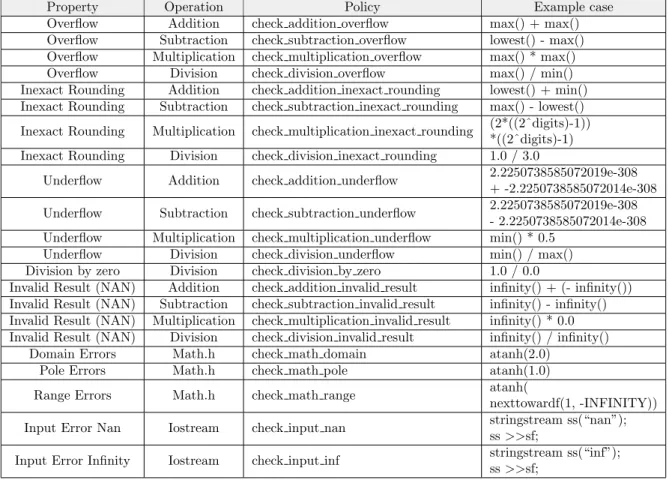
4.1 Basic set of check policies implemented in Safe-Float . . . 50
4.2 Composed check policies defined for convenience in Safe-Float . . . 52
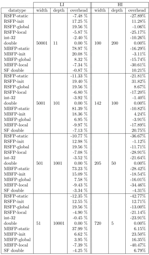
4.3 DEVStone comparing time datatypes in aDEVS . . . 70
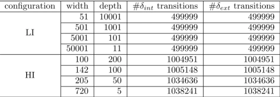
4.4 DEVStone theoretical transitions on experiments . . . 71
4.5 DEVStone comparing Safe-Float to double without compiler optimizations . . . 71
6.1 Summary of DEVS models and the DEVS subclasses they belong to . . . 103
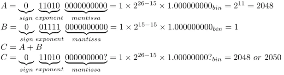
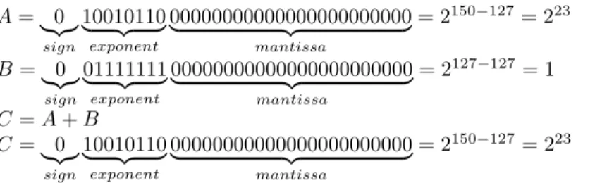
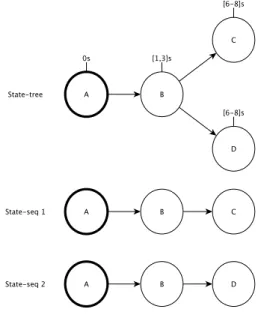
3.1 Half-precision floating-point representation examples: 2, 2.0039062, and 3.9980469 . . . . 24 3.2 Half-precision floating-point addition result example . . . 24 3.3 Half-precision floating-point representation examples: 1 and 4096 . . . 25 3.4 An example model subject to reordering errors when representing time using floating-point 28 3.5 Expected output trajectories of the example model . . . 29 3.6 Example of half-precision floating-point addition affecting DES resulting trajectories . . . 31 3.7 Example of single-precision floating-point increment affecting DES resulting trajectories . 32 3.8 Example of half-precision floating-point increment affecting DES resulting trajectories . . 33 6.1 State trajectory of non-Schedule-Preserving (non-SP) pedestrian traffic light with input
at exactly 1s . . . 84 6.2 Example of a states-tree and its expansion to state-sequences . . . 87 6.3 Example of Output and State trajectories-tree of a non-SP pedestrian traffic light . . . . 104 7.1 Architecture view of the simulator showing the PDEVS simulation components . . . 110 7.2 Model classes . . . 111 7.3 Execution classes . . . 112 7.4 Experiment on LI configuration with Width = 1000, Height = 5, and Individual Events . 113 7.5 Experiment on HI configuration with Width = 100, Height = 5, and Individual Events . . 114 7.6 Experiment on LI configuration with Width = 1000, Height = 5, and Simultaneous Events114 7.7 Experiment on HI configuration with Width = 100, Height = 5, and Simulataneous Events115
7.9 Experiment on LI configuration with Width = 100, variable Depth, and Simultaneous Events . . . 116 7.10 Experiment on LI configuration with variable groups of Simultaneous Events . . . 116
2.1 Classical-DEVS simulator . . . 12
2.2 Classical-DEVS coordinator . . . 13
2.3 Parallel-DEVS (PDEVS) root-coordinator . . . 15
2.4 PDEVS coordinator . . . 16
2.5 PDEVS simulator . . . 17
6.1 Model of a non-Schedule-Preserving pedestrian traffic light . . . 85
6.2 Abstract Simulator for atomic models allowing input with occurrence uncertainty . . . 88
6.3 Main-loop advancing on a No-Collision scenario . . . 91
6.4 Main-loop advancing on a Input-Collision scenario . . . 93
6.5 Main-loop advancing on a Scheduled-Collision scenario . . . 95
6.6 Main-loop for coordinating simulation using measured input . . . 95
7.1 Sequential PDEVS Coordinator . . . 108
7.2 Sequential PDEVS Simulator . . . 109
4.1 Example of continue execution unaware of a domain error . . . 41
4.2 Example of detecting a domain error with Safe-Float . . . 42
4.3 Example of continue execution unaware of a pole error . . . 42
4.4 Example of detecting a pole error with Safe-Float . . . 42
4.5 Example of continue execution unaware of a range error . . . 43
4.6 Example of detecting a range error with Safe-Float . . . 43
4.7 Example of continue execution unaware of a int to float approximation . . . 44
4.8 Example of detecting a int to float approximation with Safe-Float . . . 44
4.9 Example of continue execution unaware of a float to int out-of-range assign . . . 44
4.10 Example of detecting a float to int out-of-range assign with Safe-Float . . . 44
4.11 Example of continue execution unaware of an incorrect narrowing . . . 45
4.12 Example of detecting an incorrect narrowing with Safe-Float . . . 45
4.13 Example of continue execution unaware of an unexpected approximation . . . 46
4.14 Example of detecting an unexpected approximation with Safe-Float . . . 46
4.15 Example of continue execution unaware of a NaN introduced from stream . . . 47
4.16 Example of detecting an infinite being read from a stream with Safe-Float . . . 47
4.17 Example of continue execution unaware of operating with denormal values . . . 48
4.18 Example of detecting the use of a denormal value with Safe-Float . . . 48
4.19 Compose-check implementation for Safe-Float check-policy combinations . . . 51
4.20 Example of enabling a cast method in Safe-Float . . . 52 xv
4.22 RSFP-init . . . 58
4.23 RSFP-local . . . 60
4.24 RSFP-global . . . 60
5.1 Irrational time . . . 76
2.1 Example of a continuous system with Zeno problems . . . 8
4.1 Rational-Scaled floating-point (RSFP) interpretation . . . 55
4.2 Example of representing 3 ns in RSFP . . . 55
4.3 Example of Integer to RSFP conversion . . . 55
4.4 Example of floating-point (FP) to RSFP conversion . . . 56
4.5 Example of comparing two RSFP variables which scale-factor agreement cannot be found 63 4.6 Example of RSFP representation redundancy . . . 64
4.7 Multi-Base floating-point (MBFP) interpretation . . . 66
4.8 Example of half-precision floating-point conversion to Multi-Base floating-point (MBFP) . 66 4.9 Example of a successful Rational-Scaled floating-point (RSFP) conversion to MBFP . . . 67
4.10 Example of an RSFP value non-convertible to MBFP . . . 67
4.11 Example of adding two MBFPs . . . 68
5.1 Irrational datatype interpretation . . . 74
5.2 Property for irrationals having unique representation . . . 76
5.3 Representation for√72 . . . 78
5.4 Proof that addition of square root is rational only if radicands are perfect squares . . . 79
5.5 Proof that addition of square roots of integers can produce a new class of irrationals . . . 79
5.6 Proof that adding square root of inverses is irrational . . . 79
5.7 Proof that addition of square roots of rationals can produce a new class of irrationals . . . 80 xvii
6.2 Input-Collision predicate . . . 92
6.3 Scheduled-Collision predicate . . . 94
6.4 Every simulation step is characterized by at least one scenario (Theorem 1) . . . 96
6.5 Every simulation step is characterized by at least one scenario (Theorem 1 expanded) . . 96
6.6 A simulation step can be characterized by more than one scenario (¬ Theorem 2) . . . 97
6.7 A two states δext with infinite discontinuities . . . 99
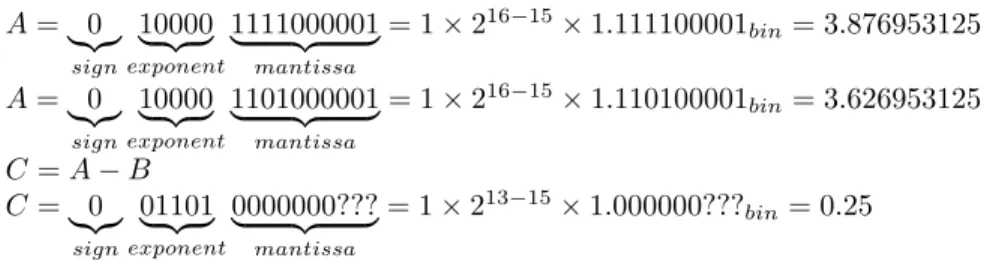
6.8 External transition functions of the example atomic models A and B . . . 101
6.9 External transition function of model C, a closure equivalent atomic model . . . 101
BIPM Bureau International de Poids et Mesures. 20, 21, 54, 82 CPU Central Processing Unit. 48, 69
DEDS Discrete-Event Dynamic Systems. 2
DES Discrete-Event Simulation. v, xii, 2–7, 9, 10, 19–21, 23, 24, 26, 27, 29–33, 40, 41, 54, 69, 72, 73, 82, 83, 106, 117, 118
DEVS Discrete-Event System Specification. xi, xiv, 2, 3, 5, 6, 9–14, 18–20, 24–28, 31, 35, 53, 54, 56, 62, 72, 73, 75, 81, 83, 86, 87, 98–101, 103, 105, 106, 109, 113, 117–119
DTS Discrete-Time Simulation. 83
FD-DEVS Finite & Deterministic DEVS. 18, 103, 105 FEL Future Events List. 28, 107, 110–112
FF-DEVS Finite-Forkable DEVS. 5, 6, 99–103, 105, 118, 119
FP floating-point. v, xii, xvii, 3, 23–35, 37, 40–49, 53–56, 65, 66, 68, 72, 73, 117 GCD Greatest Common Divisor. 36, 61, 65, 67
HI High-level of Input coupling. xii, 69, 113–115 LCM Lowest Common Multiple. 61, 65, 67
LI Low-level of Interconnections. xii, xiii, 68, 69, 113–116
MBFP Multi-Base floating-point. xvii, 39, 55, 66–69, 71, 74, 117, 118 NaN Not-a-Number. 33
non-SP non-Schedule-Preserving. xii, xiv, 84, 85, 103, 104
PDEVS Parallel-DEVS. xii, xiv, 5, 6, 14–18, 20, 24, 26, 31, 53, 106, 108–110, 113, 115, 118 xix
RSFP Rational-Scaled floating-point. xvi, xvii, 39, 55–57, 59–61, 63–69, 74, 117, 118 RT-DEVS Real-Time DEVS. 18
RTA-DEVS Rational Time Advance DEVS. 18, 38, 72 SF Safe-Float. xi, xv, 39–54, 56, 69, 71, 117
SP-DEVS Schedule Preserving DEVS. 18, 103, 105 Sym-DEVS Symbolic DEVS. 18, 38, 73
Introduction
Since we are born, we try to figure out how the world around us works, how to interact with it and how to predict the responses of the world to our stimulus. The first approach we develop is the experimental one. In this approach, we repeat and refine experiments until obtaining the desired result. For example, this is the process we follow to learn to walk and talk.
At some point in our lives, our curiosity leads us to start thinking of problems that are theoretically or practically impossible to solve using the experimental approach. For example, when sending a robot to Mars, it would be extremely expensive to start sending robots up until one arrives to Mars, or, if we want to know the age of the Sun, we cannot measure its initial value. These cases need to be studied in abstract. In order to do that, different Modeling techniques were invented.
A model is the abstract representation of an entity we want to study. As an abstraction, the model cannot capture all the properties of the studied entity. The same entity may be modeled differently to study different problems. For example, when studying how strong can be the hit of a hammer, we may not model its color, and when we are studying its kinematics, we may not model the weight of its pieces. In both cases, we are modeling a hammer, but the model in each is intended to answer different questions. A good model should focus on the properties considered important for the study in which it will be used.
Once the experiments are modeled properly, the results obtained experimenting in the abstract world can be interpreted to predict the results of similar experiments in reality. If the experimentation is reproduced in reality and the results do not match the interpretation we are in presence of an invalid model.
The analytical method for modeling, defined centuries ago, uses equations developed for reasoning over experimental results, observation and axioms previously defined. An example of this approach is the mechanics equations defined by Newton. In this method, it is usually hard to formulate equations for new systems, and when the equations are defined, it may be too complex to solve them.
In general, for cases where the models are properly defined and the methods to solve the equations 1
are known, its too complex scaling composing models. For example, the equations defined for Newtonian mechanics can be easily applied to study the interaction between two pieces in a car. Nevertheless, it might be impossible to compose the equations to study the transfer of movement from the explosion inside the engine all way through the wheels of the car describing the position of each piece participating. Models defined and studied using analytical methods provide good results for many continuous systems. These models were usually appropriate for studying phenomena in nature. Nevertheless, they are not good for human defined systems as transit, integrated circuits, or computers, which are intrinsically discrete. New methods needed to be developed for this kind of analysis.
In the last century, the introduction of computers allowed to work with symbolic manipulations that are more complex. These symbolic manipulations allowed the study of models through the generation of traces of their dynamic behavior helping to understand the evolution of the real system. We call Simulation the generation of these traces, and the device to run these algorithms a simulator. The simulator can be a person, a mechanical machine, a computer, a grid of computers, or anything achieving the goal of executing the models. The results obtained by simulating help to understand the dynamic behavior of the original system, and to produce conclusions.
To improve collaboration, sharing, and reuse about the models and simulations developed, several modeling formalisms had been proposed. Some of them are more convenient than others for each project. These formalisms can be classified according to the representation used for their time and state variables; each of these variables is classified as discrete or continuous.
In [Wai09], the modeling formalisms are classified in four groups:
• The group of formalisms representing time and state with continuous variables, known as Contin-uous Variable Dynamic Systems; an example of this could be those models defined by differential equations.
• The group of formalisms representing time with discrete variables and state with continuous ones, known as Discrete Time Dynamic Systems; an example of use is the study of sampled electronic devices signals.
• The group of formalisms representing state and time with discrete variables, known as Discrete Dynamic Systems; an example of use is the modeling of digital computers with clocks providing synchronism.
• Finally, the group of formalisms representing state with discrete variables and time with continuous ones, known as Discrete-Event Dynamic Systems (DEDS); an example of use is the modeling of a traffic light with pedestrians’ call button, which can be pushed at any time in a continuous real timeline.
In the context of this thesis, we focus our research in Discrete-Event Simulation (DES), the simulation of DEDS models. We have special interest in the family of Discrete-Event System Specification (DEVS) formalisms [ZPK+76, ZPK00].
the 70s. In DEVS, basic models are defined by their internal behavior and how they react to external inputs. These basic models can be hierarchically composed to produce models that are more complex. The algorithms for the simulation are independent of the models, and several computer simulators implementing them were developed in several architectures including distributed, parallel, sequential, object oriented, and functional. We cover the details of the DEVS modeling specification and simulation algorithms on Chapter 2.
It was proved for a large quantity of Modeling and Simulation formalisms that they model a strict subset of what DEVS can model. For most of those formalisms, translation methods are known. Using these translations, models originally developed in different formalisms can be hierarchically combined, to produce models that are more complex. Here, DEVS has the role of being the glue between formalisms for multi-formalism simulation [MZRM09].
The datatype for state variables is usually defined as part of the model and the simulator algorithms do not operate with these variables. Opposite is the case of time variables; the simulator has to interact actively with them for reproducing the chronology of events over R+, which is usually represented by
approximated datatypes as floating-point (FP). The approximation of time values in the simulation can affect the timeline preventing the generation of correct results. In addition, the existence of incomputable numbers prevents us from finding a datatype able to represent complete segments in R.
For the most popular formalisms, several implementations have been developed in various languages and platforms (we present a survey of the datatypes used by eleven popular open source DES simulators in Chapter 3). These simulators usually represent time with one of the following datatypes: FP, fixed-point, Integer, or Integer tuples. These datatypes are conveniently implemented in processors, or they are easily implementable combining native ones. Nevertheless, these datatypes have limitations in their usage that need to be noticed.
Working unaware of these limitations can be translated into issues affecting the correct generation of simulation timeline. These issues can be classified as time shifting errors, event reordering errors, and Zeno problems.
Furthermore, for DES, these errors can break the causality chain of the simulation [Lac10]. In DES, the state of the simulation can be thought of as a function of its history, producing a causal relation between them. When an event in the history is approximated, it may diverge the resulting trajectory of events. When this happens, we say that the causality chain was broken. Thus, the results obtained from the simulation are incorrect.
Current simulator implementations are silent about these errors, usually because it is impossible to detect them properly using their time datatypes. For example, when using the FP arithmetic im-plemented in the processor hardware, if no mechanism is available to notify about rounding, then the hardware outputs a value as accurate as possible.
Literature proposes some alternative approaches to be used, as rational interval datatypes, or sym-bolic algebra. This approaches have limitations too. We discuss them in Chapter 3.
computable irrational numbers. Only the rational interval and the symbolic algebra approaches attempt to represent them. However, neither of them can compare close values, and the second only supports non transcendental numbers. This restricts the set of models and simulations to those never using simultaneous events.
Another problem of interest when studying timelines is related to the uncertainty of the represented time lapses. In general, models could be simulated to predict future phenomena based on data collected in reality. When collecting data to define the models, measuring instruments and procedures are used. These instruments usually have a known associated precision. For example, a micrometer is an instru-ment designed to measure distance with 1 micron precision; when it is properly calibrated every measure taken with could have, i.e., an associated uncertainty of 1 micron; in this case, when the instrument indicates 99 microns, we could assert that the real value is between 98 and 100 microns. Sometimes, in engineering and experimental research, answering a question requires evaluating all the possible values of the measured magnitude.
Likewise, when working with continuous systems [Hoo99], there are methodologies to propagate errors widely studied in calculus and numerical methods. Mathematical tools exist to estimate the error of the output based on the error associated to the input. In discrete time systems, obtaining all the possible results starting from an imprecise input is as easy as evaluating every value in the error interval. This is possible because these systems have only a finite set of time points in each error interval.
Nevertheless, none of these methods exists in DES mathematical tools, making it impossible nowadays to track uncertainties in simulation of DES models. The tools defined for continuous systems cannot be used for DES having discrete states. Nor can the approach taken in discrete time systems because it is possible for uncertainty intervals in DES timelines to include infinite values in R.
1.1
Thesis Objectives
Considering the problems discussed above, the goals of this thesis are to devise a set of data structures and algorithms for handling representation of time properly in DES. We also want to define a method for simulating DES models and feeding them with input events having uncertainty in their time component. For the first goal, the new datatypes should provide proper representation of time for simulating without producing timeline errors, should include representation for numbers with periodicity, and should include subsets of necessary computable irrational numbers.
The algorithms provided should be able to handle input events with uncertainty in their time compo-nent for predicting future phenomena based on measures obtained in the real world. In addition, it should provide the tools to carry these errors through the model simulation. The results of these simulations should generate multiple outputs depending on the uncertainty intervals of the input. After simulating, tracing the origin of each output should be possible. We need this mechanism for understanding how an adjustment of the precision of inputs may alter the obtained results.
1.2
Thesis Contributions
The main contributions of this thesis include:
• The definition of new datatypes for representing time in DES properly for producing correct tra-jectories, supporting customizable subsets of computable irrational numbers.
• The definition of simulation algorithms for simulating every possible trajectory of a DEVS model when uncertainty quantified input events are introduced, and a subclass of DEVS models where these algorithms can be computed with finite forks in each simulation step.
• The study of a new architecture for sequential DEVS/Parallel-DEVS (PDEVS) simulators, and the implementation of such architecture in a new efficient DEVS simulator for studying its performance. As a result of this research, the following articles have been published or submitted for publication: • Dami´an Vicino, Olivier Dalle, and Gabriel Wainer. Using DEVS models to define fluid based µTP model. Poster session presented at SIGSIM-PADS 2013; Montreal, QC, Canada. This poster proposes a DEVS model for large-scale peer-to-peer file sharing networks using µTP protocol. • Dami´an Vicino, Olivier Dalle, and Gabriel Wainer. A datatype for discretized time
representa-tion in DEVS. In Proceedings of the 7th Internarepresenta-tional ICST Conference on Simularepresenta-tion Tools and Techniques, pages 11–20. ICST (Institute for Computer Sciences, Social-Informatics and Telecom-munications Engineering), 2014; Lisbon, Portugal. This paper presents the first datatype proposed for precise time and an empirical performance comparison showed.
• Dami´an Vicino, Chung-Horng Lung, Gabriel Wainer, and Olivier Dalle. Evaluating the Impact of Software-defined Networks’ Reactive Routing on BitTorrent Performance. In proceedings of SDN-NGAS 2014; Niagara Falls, ON, Canada. This paper studies the behavior of BitTorrent file propagation on emulated Software-Defined Networks.
• Dami´an Vicino, Chung-Horng Lung, Gabriel Wainer, and Olivier Dalle. Investigation on software-defined networks’ reactive routing against BitTorrent. Journal paper in IET Networks 2015/4. This paper is an extended version of the previous, comparing behavior of BitTorrent in SDN against the behavior of HTTP protocol when used in the same context.
• Mandeep Kaur Guraya, Rupinder Singh Bajwa, Dami´an Vicino, and Chung-Horng Lung. The Assessment of BitTorrent’s Performance Using SDN in a Mesh topology. Poster session presented in the sixth international conference on network of the future (NOF15); Montreal, QC, Canada. This paper explores if the results obtained in previous papers is reproducible in the mesh topology. • Dami´an Vicino, Daniella Niyonkuru, Gabriel Wainer, and Olivier Dalle. Sequential PDEVS archi-tecture. In proceedings of SpringSim15-TMS/DEVS, 2015; Alexandria, VA. This paper presents the current architecture, implementation and experimentation of the CDboost simulator.
• Dami´an Vicino, Olivier Dalle, and Gabriel Wainer. Extending Discrete-Event System Specification simulator to support metrical systems. Poster session presented at SIGSIM-PADS 2015; London, England. This poster presents the problem of introducing events with uncertainty in the time component into simulations and defines the Finite-Forkable DEVS (FF-DEVS) models’ class.
• Dami´an Vicino, Olivier Dalle, and Gabriel Wainer. Using Finite-Forkable DEVS for Decision-Making Based on Time Measured with Uncertainty, In Proceedings of the 8th EAI International Conference on Simulation Tools and Techniques 2015; Athens, Greece. This paper compares FF-DEVS against other subclasses of FF-DEVS, and introduces the simulation algorithms.
1.3
Structure of the Thesis
The rest of this thesis is organized as follows. In Chapter 2, we review the state of the art of the literature and the main concepts used. This review includes time representation, computable numbers, Discrete-Event Simulation, and Measurement Uncertainty topics.
In Chapter 3, we review current datatypes used in computer simulators. We describe these datatypes limitations, and classify how these limitations can affect the timeline of the simulation.
In Chapter 4, we propose four new datatypes for detecting and preventing errors in timelines. We describe the usage scenarios for each of them. And, we end the chapter with an empirical performance evaluation.
In Chapter 5, we proposed a method for supporting irrational numbers in DES timelines.
In Chapter 6, we propose a method for simulating DES models considering input with uncertainty. In addition, we define a subclass of models that could be simulated using this method for any input.
In Chapter 7, we present a sequential architecture for implementing PDEVS simulators. We describe our implementation in C++11 of this architecture. And, we compare it against other simulators using the DEVStone benchmark.
Background
2.1
Time representation
Foundational work about Time representations in computers was developed in the 70s and 80s. These works were focused on studying problems related to the synchronization of distributed systems and real time applications [GHJ97]. Lamport formalized time [Lam78] for distributed systems, defining it as a sequence of partially ordered events using the relation “happened before”. Later, formal approaches were proposed based in temporal logic [MMP92, MP92]. Temporal logic allows specifying constraints between events and continuous intervals of time. Using temporal logic, it is possible to reason about time constraints and provides formal proofs to properties, datatypes, and algorithms as those explained in Chapter 1.
In [All81, All83], an interval-based representation for time is proposed. This approach defines five relations between the time intervals to be considered: before, equal, meets, overlaps, and during; com-plementary relations are defined to reach a complete set of thirteen relation operations. In this work, a definition of “now” is provided together with decision algorithms for interpreting information represented using time intervals.
In 2009, Clock Constraint Specification Language (CCSL) [And09] was proposed as a standard to extend the Unified Modeling Language (UML). This new addition is used to describe relations between time instants in dense and discrete time representations. The specification language allows a definition of clocks and relations between them. Using these clocks and relations, formal proofs can be obtained on the behavior of a specified system. The goal of the project is the use of automated model checking tools in systems having time semantics, i.e., simulators.
In modeling and simulation, it is common to allow the definition of instantaneous or close to instan-taneous actions. Allowing this kind of actions may lead to Zeno conditions [Lee14], which means that it is possible to have infinite actions in a finite period.
Zeno behavior is not limited to Discrete-Event Simulation (DES), which we discuss in Section 2.4; 7
it is also possible in continuous systems. In [Lee14], the continuous system described by Formula 2.1 is proposed. This (continuous) function produces infinite oscillations when evaluated with t between 0 and 1.
x : R→ R x(t) = sin( 2πt
1− t) if 0≤ t < 1 x(t) = 0 otherwise
Formula 2.1: Example of a continuous system with Zeno problems
2.2
Computable Numbers
Alan Turing introduced computable real numbers in his foundational paper ‘On Computable Numbers, with an Application to the Entscheidungsproblem’ [Tur36]. He defines: ‘The computable numbers may be described briefly as the real numbers whose expressions as a decimal are calculable by finite means’. Different authors provided several equivalent definitions, for example, an alternative equivalent definition is ‘a number is computable if there exist an algorithm to produce each digit of its decimal expansion and for any digit requested it finishes the execution successfully’ [Abe01]. There are subsets of real numbers that had been proved non-computable. Examples of such a subset include the family of Chaitin’s constants [Cha75].
A new area of applied mathematics was developed based on the theory of computable real numbers, called Computable Calculus [Abe01]. The main goal of this area is spotting the adjustments that need to be done to theorems and properties on real calculus that does not apply to computable real numbers. For example, since an algorithm can describe each computable number, the set of computable numbers is countable, while real numbers are not [Tur36].
Some interesting results in Computable Calculus are the following non-decidable problems in ‘Com-putable Calculus’ by Oliver Aberth [Abe01]:
• In the general case, it is impossible to decide if a computable real number is irrational or not. This is because to be certain about numbers periodicity, it is necessary to check every digit of the numeric expansion, which may be infinite.
• In the general case, it is impossible to decide if a computable real number is greater than zero or equal to zero. It is possible to say that a number is not zero as soon as the first digit different from zero appears in its digit expansion, but there is no guarantee this will ever happen. When the number is effectively zero, infinite digits might need to be checked, which is impossible by finite means. In the case of comparison for greater than zero, the same argument can be used: there is no way to find out if the number is slightly greater than zero or if it is effectively zero in finite steps.
instance the equality of two numbers and the order of two numbers. This is because if they were solvable, we could subtract the two numbers and it will allow us to solve the previous problems. Detailed proofs of these non-decidable problems can be found in [Abe01].
To operate with computable numbers, we can use interval arithmetic based on the k-digits decimal expansion of the considered number N , noted N0, and the number N1obtained by adding ‘1’ to its last
digit, these numbers can be used as borders of an interval representing the considered number N [Abe01]. In interval arithmetic, the addition of two intervals is defined as the interval where lower end is defined by the addition of the two lower ends and higher end is defined by the addition of the two higher ends [Moo66]. Similar definitions exist for other operations as subtraction, multiplication and division [Moo66].
The definition of comparison operations of intervals is more complicate because the two intervals being compared may intersect; this is why multiple comparison operations need to be defined for them [Abe01, Moo66, All83].
In the case of DES, most simulation is advanced adding time values, and deciding which event to process next. In particular, if we analyze the Discrete-Event System Specification (DEVS) family simulation algorithms proposed by Zeigler [ZPK+
76], when using intervals to approximate computable numbers it is enough to define the equality and lower than compare operators for intervals that do not intersect [Abe01]. In the case the intervals approximating two numbers overlap, it is impossible to decide comparison for the numbers being approximated based in the current approximation.
When algorithmic definitions of computable numbers are available, they can be used to get a more accurate approximation, and to compare again using smaller intervals to reduce the possibility of inter-section.
If there is a chance that the numbers are equal we have no way to detect it in the general case. Thus we could keep reducing the interval indefinitely without obtaining any definitive result [Abe01].
2.3
Discrete-Event Simulation
Discrete-Event Simulation (DES) is a technique in which the simulation engine plays a history following a chronology of events [ZPK+76, ZPK00, Wai09]. The technique is called ”discrete-event” because the
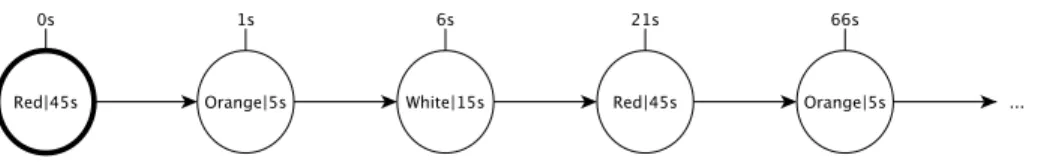
processing of each event of the chronology takes place at discrete points of a timeline. The virtual time of the simulation does not require any synchronization with real time. This allows us to predict future phenomena or study complex process happening in a short time. Unless the system being modeled already follows a discretized schedule (i.e., in the case of basic traffic lights), the process of modeling a phenomenon using a discrete-event simulator can be considered as a discretization process.
In the earlier days of DES, multiple modeling and simulation languages were developed, such as the popular SIMULA [DN66]. Most of these languages lacked of formal soundness [Nan81]. The
ear-liest approaches for formalizing DES added time semantics to well-known static modeling approaches as Timed-Automata [AD94], and Generalized Semi-Markovian Processes (GSMP) [Gly89]. Others for-malisms focused on concurrency problems emerged at the time, i.e. Petri-nets [Pet81], Calculus of Communicating Systems (CCS) [Mil80], and Communicating Sequential Processes (CSP) [Hoa78].
Among the many DES techniques, we are interested in the DEVS formalism [ZPK+76, ZPK00], which
provides a theoretical framework to think about Modeling using a hierarchical, modular approach. This formalism is proven universal for DES modeling, meaning that any model described by other DES formalism has an equivalent model in DEVS. Other characteristic of DEVS is the clear separation between model and simulation: models are described using a formal notation, and simulation algorithms are provided for running any model.
Nowadays, the DEVS term is not only used to designate a specific formalism, but more generally, to designate a family of formalisms derived from the original DEVS. For the sake of clarity, we will call the first developed DEVS formalism Classical-DEVS [ZPK00] from now on.
2.3.1
Classical-DEVS
Classical-DEVS, originally DEVS, is the formalism proposed by Zeigler in the 70s. This formalism has been implemented in multiple languages and platforms. Some implementation examples include CD++[Wai09], DEVS++ [Hwa07], DEVSJava [ZS03], James II [HU07b], pyDEVS [BV02], and Small-DEVS [JK06].
In Classical-DEVS, the modeling hierarchy has two kinds of components: atomic models and coupled models. The atomic models are defined as a tuple: A =hS, X, Y, δint, δext, λ, tai where:
S is the set of states,
X is the set of input ports and values, Y is the set of output ports and values, δint: S→ S is the internal transition function,
Q ={(s, e)|s ∈ S, 0 ≤ e ≤ ta(s)} is the total state set (where e is the time elapsed since last transition), δext: Q× X → S is the external transition function,
λ : S→ Y is the output function, and ta : S→ R+ is the time-advance function.
An atomic model, also known as a basic model, is always in a specific state waiting to complete the lifespan delay returned by the ta function, unless an input of a new external event occurs. If no external event is received during the lifespan delay, the output function λ is called first, and then the state is changed according to the value returned by the δint function. If an external event is received, then the
state is changed according to the value returned by the δext function, but no output is generated.
For instance, a pedestrian traffic light with a call-button for crossing could be modeled as follows: S ={red, white} × R+
X ={button-pressed} Y ={red-light, white-light}
δint(hwhite, .i) = hred, 10i
δint(hred, .i) = hwhite, 5i
δext(hwhite, ti, e, button-pressed) = hwhite, t − ei
δext(hred, .i, e, button-pressed) = hred, 1i
λ(hwhite, ti) = red-light λ(hred, ti) = white-light ta(h., ti) = t
Here, the state has two components, the first for keeping record of which light is on, and the second for keeping track of how long it will take until the next change of light happens. I.e. the statehred, 1i means in a second from now, the light will switch to white.
The only input is the result of pressing the pedestrian call-button; this button is in charge of reschedul-ing the next white light. There is two possible outputs defined, red-light meanreschedul-ing that light is bereschedul-ing switched to red, and white-light meaning it is switched to white.
The internal transition function (δint) switches the state when the waiting time expires, when the
light is switched, a constant is assigned to the time component of the state. When interpreting the internal transition the time component of the state is not considered for deciding the new state. When result is independent from a variable, we mark it with a point. The external transition function (δext)
schedules the switch to white to happen in next second if the light is currently red. In case the button is pressed while the light is white, nothing is rescheduled. Depending the color of current state, the time component would be important. In the case current state is white, we preserve the scheduling of the next switch by subtracting the elapsed time to the time registered in the state. In the case current state being red, we maintain the color and change the time component to one. The output function (λ), executed right before the internal transition function signals the light being registered as new state by the internal transition function. I.e. if current state is red, output function result is white-light, which matches the new state after the internal transition function is executed. The time-advance function (ta), used for signaling how long to wait for next transition is always returning the time value of the current state.
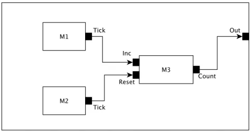
Coupled models define a network structure in which nodes are any Classical-DEVS models (coupled or basic) and oriented links represent the routing of events between outputs and inputs or to/from upper level.
Formally, a Coupled Model is represented by the tuple C = hX, Y, D, M, Cxx, Cyx, Cyy, SELECTi
where:
X is the set of input events, Y is the set of output events,
D is an index for the Classical-DEVS component models of the coupled model, M ={Md|d ∈ D} is a tuple of Classical-DEVS models as previously defined,
Cxx⊆ X × ∪i∈D(Xi) is the set of external input couplings;
Cyx⊆ ∪i∈D(Yi)× ∪i ∈ D(Xi) is the set of internal couplings;
SELECT : 2D\ ∅ → D is the tie-breaker function that sets priority in case of simultaneous events.
Alternatively, in the variant of DEVS with ports (were each model has multiple input and output ports), the coupling relations are defined using EIC, EOC, and IC notation. EIC, EOC, and IC are re-spectively the External Input Coupling, External Output Couplings and Internal Couplings that explicit the connections and port associations respectively from external inputs to internal inputs, from internal outputs to external outputs, and from internal outputs to internal inputs,
In some cases, models producing zero time-advances in their transitions could reach an infinite loop and stale the simulation. For this reason, a legitimacy rule was added to the formalism; the legitimacy rule for DEVS [ZPK00] states models must never produce infinite zero-time-advances in finite segments of its timeline to be considered legitimate.
The formalism also provides abstract algorithms of an abstract simulator for these models, which define the semantics of the simulation. In Algorithms 2.1 and 2.2, we show the algorithms for simulator and coordinator as defined in [ZPK+
76]. The simulator is in charge of simulating atomic models, while the coordinator simulates the coupled models.
Data: parent, A
// simulator variables: parent // parent coordinator tlast // time of last event
tnext // time of next event
A // the simulated atomic model s // the current state of A
When receive init-message(Time t) do tlast:= t
tnext:= tlast+ A.ta(s)
done
When receive *-message(Time t) do if t6= tnext then
error: bad synchronization end
y := A.λ(s)
send y-message(y, t) to parent s := A.δint(s)
tlast:= t
tnext:= tlast+ A.ta(s)
done
When receive x-message( X x, Time t) do if ¬(tlast ≤ t ≤ tnext) then
error: bad synchronization end
s := A.δext(s, t, t− tlast, x)
tlast:= t
tnext:= tlast+ A.ta(s)
done
Algorithm 2.1: Classical-DEVS simulator
Data: parent, N
// coordinator Variables: parent// parent coordinator tlast// time of last event
tnext// time of next event
N // the simulated Coupled model When receive init-message(Time t) do
foreach i∈ D do
send init-message(t) to child i tlast:= max{tlast[i] : i∈ D}
tnext:= min{tnext[i] : i∈ D}
end done
When receive *-message(Time t) do if t6= tnext then
error: bad synchronization end
i′= N.Select(
{i ∈ D : tnext[i] = tnext})
send *-message( t ) to i′
tlast:= max{tlast[i] : i∈ D}
tnext:= min{tnext[i] : i∈ D}
done
When receive x-message(X x, Time t) do if ¬(tlast≤ t ≤ tnext) then
error: bad synchronization end
foreach (x, xi)∈ Cxxdo
send x-message( xi, t ) to child i
tlast:= max{tlast[i] : i∈ D}
tnext:= min{tnext[i] : i∈ D}
end done
When receive y-message(Y yi, Time t) do
foreach (yi, xi)∈ Cyx do
send x-message( xi, t ) to child i
if Cyy 6= ∅ then
send y-message( Cyy(yi), t ) to parent
tlast:= max{tlast[i] : i∈ D}
tnext:= min{tnext[i] : i∈ D}
end end done
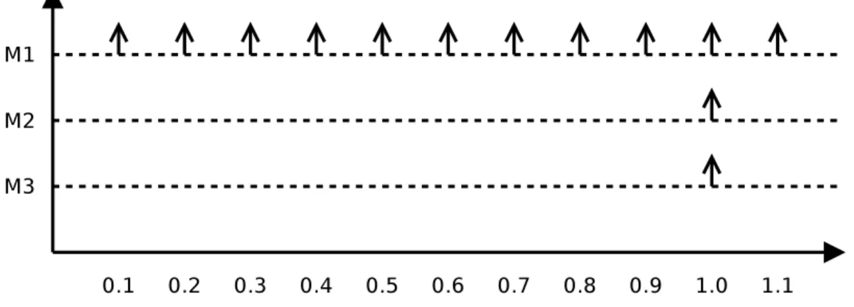
simulation engine. Simultaneous events correspond to the cases in which the discretization that results from the discrete-event modeling produces identical time values. Simultaneous events occur in DEVS in two ways: either a model receives input events from multiple models at the same time, or it receives events from other models at the same time as it is reaching the end of the time-advance delay. In this case, the tie-breaker function named SELECT is used to decide what model is simulated first.
The simulation starts from a main loop (root-coordinator), which drives the whole simulation by repeatedly sending *-messages to the topmost coordinator.
2.3.2
Parallel DEVS (PDEVS)
The Parallel-DEVS (PDEVS) [CZ94, CZK94] goal is to remove problems of serial computation caused by the SELECT function under the occurrence of simultaneous events in Classical-DEVS. To achieve this, atomic models receive bags of messages; all events in the bag are considered simultaneous. The external transition function needs to process all events in the bag at once rather than one at a time as in Classical-DEVS. In addition, a new function is included in atomic models for handling cases where internal transitions and external transitions are simultaneous. This new function is called Confluence function and has to deal with bags of external events.
An atomic model in PDEVS is specified as a tuple M =hX, Y, S, δext, δint, δconf, λ, tai where:
S is the set of sequential states, X is the set of input events, Y is the set of output events,
δextis the external transition function,
δint is the internal transition function,
δconf is the confluent function,
λ is the output function, and ta is the time-advance function.
In this specification, the confluent transition function (δconf(s, e, x)) computes the next state using
the current state s, the elapsed time e and the input events x when the internal and external events occur simultaneously. The rest of the PDEVS specification follows the Classical-DEVS specification.
A coupled model in PDEVS is specified [CZ94] as DN ={X, Y, D, {Mi}, {Ii}, {Zi,j} where:
X is the set of input events, Y is the set of output events,
D is the set of the component names,
Miis the DEVS system of component name i∈ D,
Ii is the influencers of Mi for each i∈ D and
Zi,j defines the Mi-to-Mj output translation for each i, j in Ii, and from/to upper levels.
The whole DN specification follows the Classical-DEVS Coupled specification except for the SELECT function, which is removed.
In Algorithms 2.3, 2.4, and 2.5, we show the abstract algorithms for the PDEVS simulators [CZK94]. This simulator mainly uses three types of messages: internal state transition message (*, xcount, t),
output/input message (@, content, t) and ending message (done, tnext). (*, xcount, t) and (done, tnext)
messages are for state transition synchronization. A (@, content, t) message conveys the content of an output event to its parent coordinator, which then routes the messages to appropriate influences.
The simulation starts from a main loop (root coordinator in Algorithm 2.3), which drives the whole simulation by repeatedly sending (*, 0, t) to the topmost coordinator and waiting for a done message to advance the global simulation clock to tnext.
In Algorithm 2.4, we show the algorithms for PDEVS Coordinators. Here, when an internal message (*, xcount, t) is received, it is forwarded as (*, icount, t) to all components of the coupled model members
of the imminent set (IMM) or receivers (INF).
Note that xcount originally contains the number of influencers of the coupled model, and icount will
save the total number of influencers of a component defined inside a coordinator. semaphorecount is
increased every time a *-message is sent to an inferior PDEVS component. The ending message will only be sent when semaphorecount is 0. Here, any output/input message is forwarded according to the
coupling relations Zi,j to other simulators and coordinators. In addition, when an ending message is
received, tnext(next internal event time) is saved in an event list and the internal variable semaphorecount
is decreased.
// Root-coordinator Variables: t // current time
t := tnext of the topmost coordinator
repeat
send(@, t) to the coordinator of the topmost coupled model wait until (done, tnext) is received
send(*, t) to the coordinator of the topmost coupled model wait until (done, tnext) is received
t := tnext of the coordinator of the topmost coupled model
until t =∞;
exit // simulation complete
Algorithm 2.3: PDEVS root-coordinator
In Algorithm 2.5, we show the algorithms for the PDEVS abstract simulator. Here, when a (*, xcount,
t) message is received, it indicates an event, internal or external, has to be processed.
If the simulation time reaches tnext(time of the next internal event), compute the output function and
send the output events to the parent coordinator. If semaphorecount is 0, only the internal transition
takes place, otherwise, both internal and external functions take place at the same time leading to the confluent function to be executed once semaphorecount is 0. After this, the tnext is calculated and an
ending message is sent to the parent coordinator. Here, any content of an input message (@, content, t) is saved in a vector xb (event bag) and the value of semaphorecount decreased by one. semaphorecount
will be equal to 0 when all input events at the simulation time t have been saved in the event bag xb.
// Coordinator Variables: parent// parent coordinator tlast// time of last event
tnext// time of next event
C// the coordinated coupled model
child set// set of child simulators/coordinators synchronize set bag// messages to be processed When receive @-message(Time t) do
if t = tnext then
tlast:= t
forall the imminent child processors i with minimum tnext do
send(@, t) to child i
cache i in the synchronize set end
wait until (done, t) is received form all imminent processors send (done, t) to the parent
end
raise an error done
When receive y-message(Y y, Time t) from child i do forall the all influences j of child i do
q := C.zi,j(y)
send(q, t) to child j
cache j in the synchronize set end
wait until all (done, t)’s are received from j
if self ∈ Ii then //y needs to be transmitted upwards
y := C.zi,self(y)
send(y,t) to parent end
done
When receive q-message(Event q, Time t) from parent do lock the bag
add event q to the bag unlock the bag
done
When receive *-message(Time t do if tlast ≤ t ≤ tnext then
forall the receivers, j ∈ Iself∧ all q ∈ bag do
q := C.zself,j(q)
send(q, t) to j
cache j in the sinchronize set end
wait until all (done, tnext)’s are received
tlast:= t
tnext:= min{tnext[i] : i∈ D}
clear the syncronize set send(done, t) to parent end
raise an error done
// Simulator Variables: parent// parent coordinator tlast// time of last event
tnext// time of next event
A // the simulated atomic model s // current state of A
bag // messages to be processed When receive @-message(Time t) do
if t = tnext then
y := A.λ(s)
send(y, t) to the parent send(done, t) to the parent end
raise error done
When receive q-message(Event q, Time t) do lock the bag
add event q to the bag unlock the bag
send(done, t) to the parent done
When receive *-message(Time t) do if tlast ≤ t < tnext∧ bag 6= ∅ then
e := t− tlast
s := A.δext(s, e, bag)
empty bag tlast:= t
tnext:= A.ta(s)
end
if t = tnext∧ bag = ∅ then
s := A.δint(s)
tlast:= t
tnext= tlast+ A.ta(s)
end
if t = tnext∧ bag 6= ∅ then
s := A.δconf(s, bag)
empty bag tlast:= t
tnext:= tlast+ A.ta(s)
end
if t > tnext∨ t < tlast then
raise error end
send(done, tnext) to parent
done
as Zeigler’s simulation algorithms are defined for PDEVS [HU06]. In the context of our work, we always refer to Chow’s algorithms presented in Algorithms 2.4, 2.3, 2.5.
2.3.3
Simulating by closure
Several simulators have implemented PDEVS. In particular, in aDEVS [Nut03], Nutaro takes a different approach [MN05] using the closure under coupling property of DEVS models, which states that for every coupled model it exists an equivalent atomic model [ZPK00].
Each coupled model (also referred to as network model in Nutaro proposed architecture) are reduced to an equivalent atomic model called the resultant. The resultant of a coupled model is an atomic model in which the set of states, transition functions and output functions are defined by its interconnected components. Exploiting this closure property, the resultant transformation produces a single atomic model, and hence eliminates the necessity of coordinators.
2.3.4
Other DEVS extensions
Several extensions have been proposed to DEVS. These extensions include, Fuzzy DEVS [ZPK00] pro-viding a fuzzy logic to the state definition, Symbolic DEVS (Sym-DEVS) [ZC92] using symbolic algebra to represent time, Rational Time Advance DEVS (RTA-DEVS) [SW10, Saa12] using interval arithmetic to operate timelines, and others. In this section, we describe those most relevant for our work.
Sym-DEVS [ZC92, ZPK00] was developed in early 90s; it extends the DEVS formalism to define time as linear polynomials in place of real numbers. This formalism can be used to study the fault conditions and other properties when doing model verification. Its abstract simulator examines all possible strict choices of imminent forking execution when needed.
RTA-DEVS [SW10, Saa12] is another proposed extension to DEVS formalism. In RTA-DEVS, time is defined as intervals with rational borders. The goal of this formalism is to allow only the specification of models that can be automatically verified using model checking methods. To achieve this goal, the set of specifiable models is reduced to those that never have irrational time-advances.
Schedule Preserving DEVS (SP-DEVS) [HC04] and Finite & Deterministic DEVS (FD-DEVS) [HZ06] only allow the modeling of a strict subclass of DEVS models. The restriction is applied for researching state reachability.
The FD-DEVS subclass is restricted to those models having a finite set of states and scheduling tran-sitions expressed by rational time-advances. In addition to the restrictions imposed by FD-DEVS, the SP-DEVS subclass is restricted to the models never changing scheduled transition times when receiving exogenous events.
The Real-Time DEVS (RT-DEVS) [HSKP97] was proposed for specifying simulation under real-time constraints, for example for simulation with human in the loop for training. In this formalism, actions are introduced, which have to be completed into time-windows. If an action is not reproduced before
the time-window is expired, it is discarded and the simulation goes on, like if it had never happened. Finally, in Quantized-State Systems (QSS) [KJ01], a method is proposed for simulating approxima-tions of continuous systems using DEVS.
2.3.5
The DEVStone benchmark
DEVStone [GW05, WGGA11] is a synthetic benchmark devoted to automate the evaluation of DEVS-based simulators, and it can be adapted to other DES engines. It generates a suite of models of different sizes, complexities and behaviors similar to diverse applications that exist in the real world.
DEVStone was created to study and compare the efficiency of DEVS simulators, compare different versions of a specific simulation engine, and aid the measurement and improvement of different DEVS-based software. The method proposes a theoretical time computed from the topology generated and the time required to run every transition, each executing Dhrystones [Wei84]. The execution time of the DEVStone is compared to the theoretical expected time to evaluate the overhead introduced by the simulator.
The DEVStone model generator permits one focusing on essential aspects that impact performance namely the size of the model and the workload done in the transition functions. The following parameters are used to generate a model: type (structure and interconnections between the model components), depth (number of levels in the modeling hierarchy), width (number of components in each immediate coupled model), internal transition time (execution time spent by the internal transition functions) and external transition time (execution time taken by external transition functions).
Four types of models (LI, HI, HO and HOMod) with different internal and external structure can be used:
• LI: Models with a low level of interconnections for each coupled model. Each coupled component has only one input and one output port. The input port is connected to each component but only one component produced an output through the output port.
• HI: Models with a high level of input couplings. HI Models have the same number of atomic components with more interconnections: each atomic component (a) connects its output port to the input port of the (a + 1)th component.
• HO and HOmod [WGGA11]: Models with high level of coupling and numerous outputs. HO models have two input and two output ports at each level while HOmod have a second set of (width - 1) models where each one of the atomic components triggers the entire first set of (width - 1) atomic models.
Because the model structure and the time spent in transition functions, which consume CPU clocks by running Dhrystones [Wei84] is known, the model execution time can be easily computed. Detailed computation formulas can be found in [GW05, WGGA11].
by a significant margin for large models. Several other PDEVS simulators (JAMES II, VLE, PyDEVS, and DEVS-Ruby) have been compared to aDEVS using DEVStone as well. The most recent work is by Franceschini et al. [FBT+
14] where aDEVS remains the reference with regard to performance. This has been closely followed by a recent reimplementation of PyPDEVS [VTV14].
The most common use of DEVStone is for comparing different simulators; nevertheless, it can be also used to evaluate proposed improvements to a simulator. An example was the use of DEVStone for evaluating an improvement proposed by Kim et al. in [KKSS00]. To remove performance inefficiency, flattening the model has been proposed by Kim et al.. Using this approach, the model structure is modified so that the new model has no intermediary coupled models. This approach is different from the one used in aDEVS to produce a closure resultant, it rewrites the coupling to obtain a single coupled model. The impact of flattening has also been measured using DEVStone. In [GW05], and results show a clear improvement when using the flattening approach compared to the hierarchical approach.
2.3.6
Simulators with branching
Simulators not implementing DEVS have used execution branch or fork to solve some problems in the past. Most notorious examples are in the group of Logical-Process based simulators. In [PM07] the Moose simulator is presented, this simulator does not have tie-breaking functions as DEVS. When simultaneous events are received the execution is branched to simulate the simultaneous events in all possible permutations. Each branch of simulation may lead to different results.
In [HF97, HF01] branching (or cloning) is proposed as a mechanism to advance interactive simu-lations at points where user input is “undecided”. In [HF02], optimizations to exploit repetition of information between cloned simulations and lazy-cloning ideas are presented in the context of Parallel Logical Processes simulation.
2.4
Measurement Uncertainty
One of many usages of DES is being part of a decision-making process for industrial and research works. Here, data is collected from the real system using measuring instruments and processes. From them, a set of measurement results is obtained and used as input to feed the simulation.
Metrology is the science of measurements and its applications. In this thesis, we adhere to the metrological vocabulary and practices proposed by the Bureau International de Poids et Mesures (BIPM), an international organization whose goal is to produce globally adopted metrological standards. BIPM is responsible for the standardization of the meter, gram, second and other international standardized units, for the provision of procedures and practices for properly measure in industrial and scientific works, and for the publication of other metrology related articles to advance the state of the art in the discipline.
Mea-surement [BIP08] and International Vocabulary of Metrology [BIII08] documents provided by BIPM. Mostly, we only refer to the following terms:
• Measurand [BIII08]: the quantity to be measured.
• True value [BIII08]: a theoretical value of the measurement assuming perfect accuracy, in the practice this value is unknowable.
• Measurement Result [BIII08]: set of quantity values being attributed to a measurand together with any other relevant information, generally expressed as a measurement value and a measurement uncertainty.
• Measurement Uncertainty [BIII08, BIP08]: non-negative parameter characterizing the dispersion of the quantity values being attributed to a measurand, based on the information used.
Metrology [BIII08] states it is not possible to determine true values from measuring magnitudes. For this reason, measurement results are provided with uncertainty quantifications, or error margins. The measurement result with uncertainty quantification is usually represented as an uncertainty interval for an acceptable level of confidence.
2.4.1
Uncertainty on DES
In the area of Parallel DES, uncertainty was used for speeding up simulations. On models not containing uncertainty quantifications, simulator assigns them and uses them for speeding up the simulation. Some authors have chosen to introduce uncertainty intervals for every time point in the model [LF00, LF04a, LF04b]. Any point in the intervals is considered equal for simulation purposes and selecting which one to use for running the events is based on parallelizing the execution of largest possible quantity of events. For this purpose, authors refer to the concepts of Approximate Time and Approximate Time Event Ordering [Fuj99, LF00]. In Approximate Time Event Ordering, the common ordering used is Approxi-mate Time Causal, which is defined for Events being concurrent if any point in their uncertainty intervals overlaps. For concurrent events, a second ordering is used, the causality relation “before than” [Lam78]. These approaches state that there is a relation between the simulation results accuracy and the un-certainty introduced, but they do not provide tools to bound the errors, quantify the results unun-certainty, or express qualitative information about the validity of the obtained result.
The general approach is based on the Approximated Time presented in [Fuj99]. A case study is presented in [LF04a] in the context of interactive simulation; Architectural details for process-oriented distributed simulation are also provided in [LF04b].
In [LF00] an alternative approach is described, where after assigning uncertainty to the values, a precise value is chosen from a pre-sampled set of random numbers for each event. This allows using pre-existing federated simulation tools as HLA without requiring modifications while speeding up sim-ulations. The paper also define how to constraint the uncertainty-look-ahead relation to obtain better speed-ups.
Other authors proposed to introduce uncertainty on spatial properties of the model for obtaining speed-ups [GCQ08, QB04]. Here, models are expected to have positional behavior, for example cell-phones and cell-towers for unwired communication. This approach can be combined to obtain further speed-ups with the Approximated Time approach previously mentioned.
Finally, in [BNO03], an architecture extending the Time Warp algorithm with Temporal Uncertainty is proposed. This architecture exploits uncertainty for avoiding rollbacks when the events to be rolled-back could be moved into their uncertainty interval to make them still useful.