Accurate hypocentre determination in the seismogenic zone of the
subducting Nazca Plate in northern Chile using a combined
on-
/offshore network
S. Husen,
1,* E. Kissling,2 E. Flueh1 and G. Asch3
1 GEOMAR Research Center for Marine Sciences of the Christian Albrechts University, W ischhofstrasse 1–3, D 24148 Kiel, Germany. E-mail: shusen@geomar.de
2 Institute of Geophysics, ET H-Ho¨nggerberg, Zurich, Switzerland 3 GeoForschungsZentrum (GFZ), Department 4, Potsdam, Germany
Accepted 1999 March 31. Received 1999 March 29; in original form 1998 June 18
S U M M A R Y
The coupled plate interface of subduction zones—commonly called the seismogenic zone—has been recognized as the origin of fatal earthquakes. A subset of the after-shock series of the great Antofagasta thrust-type event (1995 July 30; M
w=8.0) has been used to study the extent of the seismogenic zone in northern Chile. To achieve reliable and precise hypocentre locations we applied the concept of the minimum 1-D model, which incorporates iterative simultaneous inversion of velocity and hypocentre parameters. The minimum 1-D model is complemented by station corrections which are influenced by near-surface velocity heterogeneity and by the individual station elevations. By relocating mine blasts, which were not included in the inversion, we obtain absolute location errors of 1 km in epicentre and 2 km in focal depth. A study of the resolution parameters ALE and DSPR documents the importance of offshore stations on location accuracy for offshore events. Based on precisely determined hypo-centres we calculate a depth of 46 km for the lower limit of the seismogenic zone, which is in good agreement with previous studies for this area. For the upper limit we found a depth of 20 km. Our results of an aseismic zone between the upper limit of the seismogenic zone and the surface correlates with a detachment zone proposed by other studies; the results are also in agreement with thermal studies for the Antofagasta forearc region.
Key words: aftershocks, earthquake location, seismic tomography, subduction.
of authors have suggested that temperature may control
I N T R O D U C T I O N
the upper and lower limits of the seismogenic zone (Tichelaar Most of the world’s seismicity occurs along subduction zones, & Ruff 1993; Hyndman & Wang 1995 and references therein). and most of the largest earthquakes are generated along these They proposed a temperature of 250°C to 450 °C as a limit active margins. A closer look reveals that the very largest ones for great earthquake fault slip. A minimum temperature for are events mainly of thrust type located within the coupled initiating earthquakes is defined at 100–150°C (Hyndman & plate interface at a depth of less than 50 km (Ruff 1996). This Wang 1995), when stable sliding clays dehydrate to illite and part of the subduction zone—commonly called the seismogenic chlorite which are more frictionally unstable.
zone—represents a zone where coupling occurs between the To determine the minimum and maximum depths of the downgoing and the overriding plate. At greater depth, the stress coupled plate interface, accurate and reliable hypocentre deter-regime changes from compressional to extensional stress. The minations are needed, recorded either teleseismically or by a underlying plate tectonic mechanisms are still being debated local network. Global studies based on teleseismic data sets and depend, among other things, on the extent of the seismo- from various subduction zones (Tichelaar & Ruff 1993 and genic zone, specifically the minimum and maximum depths Pacheco et al. 1993) reveal a depth range of 35–70 km for (up-dip and down-dip limits) of this zone (Tichelaar & Ruff the transition zone from unstable to stable sliding along the 1993; Pacheco et al. 1993; Ruff & Tichelaar 1996). A number plate interface, which defines the base of the seismogenic zone. The studies failed, however, to determine the minimum depth of the transition zone, because focal depths of shallow
events recorded teleseismically strongly depend on an accurate simultaneously at different stations, all stations were run in continuous mode. The OBH also recorded with a sample knowledge of bathymetry and/or the properties of the uppermost
sedimentary layers (Wiens 1989). On the other hand, local frequency of 100 Hz.
Phase data were stored on CDROM, and routine phase networks provide accurate hypocentre locations (e.g. Maurer
& Kradolfer 1996) if additional ocean-bottom seismometers picking and localization of the events were performed with the -based package (Rietbrock & Scherbaum 1998). are included, since the upper limit of the seismogenic zone is
normally located somewhere between the trench and the Since all stations were operated in continuous mode, intensive preprocessing of the raw data was required. A total number coastline (Byrne et al. 1988).
In this paper we present the results of a study on the of 15 653 events were detected for the three-month period of the CINCA experiment using a software trigger with a LTA aftershock series of the great M
w=8.0 Antofagasta underthrust
event (Delouis et al. 1997). The aftershocks were recorded by to STA ratio of 8 and a coincidence check with at least five stations (Asch et al. 1995). To decrease the number of earth-a combined on- earth-and offshore network which was part of
the interdisciplinary CINCA1 project. Accurate and reliable quakes to a practical size and to select the most useful events, we increased the requested minimum number of stations per hypocentres were achieved by applying the concept of the
minimum 1-D model (Kissling 1988; Kissling et al. 1994). event to 15, thus further reducing the data set to 4426 events. Since we intend to achieve accurate hypocentre locations for This approach incorporates iterative simultaneous inversion
of hypocentres and 1-D seismic P- and S-wave velocity models offshore events, we use a subset of those 1650 events that were recorded during the period of OBH operation. Preliminary and thus accounts for the strong coupling between hypocentres
and seismic velocities. The highly accurate hypocentres are hypocentre locations for this period of 28 days are shown in Fig. 2. During phase picking, the event’s local magnitude ML used to estimate the upper and lower limits of the seismogenic
zone for the Antofagsta area. was determined by averaging the maximum peak-to-peak amplitude on one of the horizontal components for all available observations. For the subset of 1650 events, local magnitudes
The CINCA Seismic Network
range from 0.7 to 5.85 with an average of 2.37. The CINCA Seismic Network was planned and carried out
by the SFB 2672. It was a continuation of the PISCO∞943
A C C U R AT E H Y P O C E N T R E L OC AT I O N S
experiment to the west (Asch et al. 1994). As part of the CINCA project it was planned to monitor the seismicity in
an area around the city of Antofagasta over a three-month The coupled hypocentre velocity problem
period (August–September 1995). The network was originally
The traveltime of a seismic wave is a non-linear function of designed to consist of 22 PDAS recorders with 1 Hz
three-both the hypocentral parameters and seismic velocities sampled component seismometers The situation changed when, 10 days
along the ray paths between stations and hypocentre. This before the experiment started, a magnitude M
w=8.0 earth- dependence on hypocentral parameters and seismic velocities is quake (Delouis et al. 1997) struck the area around the city of
called the coupled hypocentre–velocity model problem (Crosson Antofagasta on 1995 July 30. Owing to the expected aftershock
1976; Kissling 1988; Thurber 1992). It can be linearized and series, the German Task Force for Earthquakes of the GFZ
written in matrix notation as (Kissling et al. 1994) Potsdam decided to install an additional 13 REFTEK
recorders, so that an average of 35 stations were operating t=H+Mm+e=Ad+e , (1) throughout the experiment. The network was maintained by
the GeoForschungsZentrum (GFZ) Potsdam and the Free where t is the vector of traveltime residuals (differences between observed and calculated traveltimes); H is the matrix of University of Berlin (FUB). Nine ocean-bottom hydrophones
(OBHs) complemented the network offshore over a period of partial derivatives of traveltime with respect to hypocentral parameters; h is the vector of hypocentral parameter adjust-28 days. The OBHs were deployed and recovered by GEOMAR
using the research vessel SONNE in two legs of 15 and ments; M is the matrix of partial derivatives of traveltimes with respect to model parameters; m is the vector of velocity 13 days each.
Land stations were placed along the coast within the Coastal parameter adjustments; e is the vector of traveltime errors, including contributions from errors in measuring the observed Cordillera and the Longitudinal Valley (Fig. 1). The Coastal
Cordillera represents the remnants of the former Jurassic traveltimes, errors in the calculated traveltimes due to errors in station coordinates, use of the wrong velocity model and volcanic arc, which has migrated 300 km to the east since its
formation (Scheuber et al. 1994). The OBHs were deployed hypocentral parameters, and errors caused by the linear approximation; A is the matrix of all partial derivatives; offshore on the continental slope between trench and coastline.
In total, the network covers an area of 340 km by 210 km. and d is the vector of hypocentral and model parameter adjustments.
All onshore recording sites were equipped with
three-component seismometers (MARK L4–3D, 1 Hz), and each In standard earthquake localization, the velocity para-meters are kept fixed to a priori values—which are assumed channel was recorded at 100 Hz sample frequency. Because
there is no way to check if a signal has been observed to be correct—and the observed traveltimes are minimized by pertubating hypocentral parameters. Neglecting the coupling between hypocentral and velocity parameters during the
1 Crustal Investigations on- and offshore Nazca plate and Central
location process, however, can introduce systematic errors
Andes.
(Thurber 1992; Eberhart-Phillips & Michael 1993) in the
hypo-2 Collaborative Research Group hypo-267, Deformation processes in the
centre location. Furthermore, error estimates strongly depend
Andes.
Figure 1. Network design of the CINCA experiment with main geomorphological units (MJ: Mejillones Peninsula). The contour interval of topography is 1000 m. The Trench is marked by the –7000 m isoline. The epicentre of the Antofagasta main shock is taken from the NEIC catalogue.
1995b). Precise hypocentre locations and error estimations geology. As a result of the mostly long ray paths and limited azimuthal ray distribution, station corrections in the outer therefore demand the solution of all unknowns in the coupled
inverse problem, namely the hypocentral parameters and the regions of the network contain velocity information about the shallow subsurface and linear effects of the deep structure. The velocity field. In the minimum 1-D model this will be achieved
by simultaneously inverting for hypocentre and velocity para- applicability of the concept of the minimum 1-D model even in areas of significant Moho topography and dipping structures, meters (Kissling 1988). The minimum 1-D velocity model
obtained by this trial-and-error process represents the velocity and its performance for high-precision earthquake location have been tested and documented by relocating shots and model that most closely reflects the a priori information
obtained by other studies, for example refraction studies, and mine blasts (Kissling 1988; Kradolfer 1989; Kissling & Lahr 1991; Solarino et al. 1997). In addition, no significant and that leads to a minimum average of RMS values for all
earthquakes (Kissling et al. 1995b). Each layer velocity of the systematic shift in hypocentre locations is observed after a 3-D inversion when using the minimum 1-D model as the initial minimum 1-D model is the weighted area-wise average over all
rays in the data set within that depth interval. To account for reference model (Kissling 1988; Kissling & Lahr 1991; Graeber 1997). Thus, the minimum 1-D model concept is the most lateral variations in the shallow subsurface, station corrections
are incorporated in the inversion process. For stations with an appropriate for uniform high-precision earthquake localization in the CINCA experiment, outperforming any 2-D or 3-D even azimuthal ray distribution, that is to say in the middle of
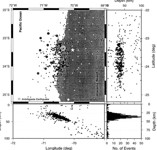
Figure 2. Seismicity over a one-month period as observed by the CINCA network extended offshore with OBHs. Events have been located routinely using a preliminary velocity model. The white star marks the position of the Mantos Blancos Mine, blasts from which will be used for determining location accuracy.
This unusually large thickness of the top layer, however,
Minimum 1-D velocity model for the CINCA experiment
introduces instabilities into the inversion procedure. In Fig. 3, velocity models as obtained by the inversion are repre-Data quality is of great importance for the success, efficiency,
and accuracy of an inversion process. To establish a set of sented by bold lines, and the initial models are plotted with grey lines. Even at intermediate depth, where good resolution events that can be accurately located, we select only those
events out of the presently available set of some 1650 earth- is expected because of adequate ray coverage, no convergence among the final velocity models can be observed. Since quakes (Fig. 2) that have an azimuthal gap of observations
(GAP) of less than 180° and at least 10 P observations. This the first kilometres within the earth crust generally show a strong velocity gradient, an unrealistic thick top layer reduces the data set used for the P-wave inversion to a total
number of 600 events. with a constant velocity as required by may intro-duce a systematic error, which would explain the observed The calculation of a minimum 1-D model is a trial and error
process starting with a wide range of realistic and possible instabilities. In an alternative approach, we neglected the station elevations and were thus able to use a more detailed unrealistic velocities as initial guesses. The use of a wide range
of velocities guarantees that all possible solutions are taken velocity discrimination in the upper layers. The omission of station elevations will, however, result in a systematic ‘error’ into account. The software routine (Kissling et al.
1995a) used for the calculation of the minimum 1-D model for the calculated traveltimes. For well-locatable events such as those in our selected data set, however, these systematic allows for station elevation, which implies that the rays
are traced exactly to the true elevation position during the errors will primarily affect the station corrections (Kissling et al. 1994; Maurer & Kradolfer 1996). Differences in ray paths forward modelling. This is an important constraint for the
CINCA experiment, where we encounter stations at elevations are negligible if focal depths of events are much larger than station elevations and in areas of strong vertical velocity of 2200 m above sea level to 5500 m below sea level yielding
a station topography of nearly 8 km. Since the ray tracer gradient, because rays travel nearly vertically beneath the stations. Station corrections in such a minimum 1-D model, currently implemented in demands that all stations
must be located within the first layer, the velocity models however, include the effects both of station elevations and of local subsurface velocity.
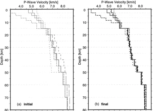
Figure 3. Initial (a) and final ( b) 1-D velocity models after inversion with station elevations. Note the poor convergence of the velocity models due to the large thickness of the top layer.
Fig. 4 shows various velocity models with refined upper Owing to intrinsic ambiguities of the inverse coupled hypocentre–velocity problem, additional boundary conditions layer thickness. Initial models are represented by grey lines
(Fig. 4a), and final velocities by bold lines (Fig. 4b). The new are needed to select a specific velocity model. In the area around Antofagasta, a refraction profile along the Coastal results—without using the station elevations—show a more
consistent behaviour. Below 15 km depth we observe a good Cordillera was interpreted by Wigger et al. (1994). Since most of the selected earthquakes are located beneath the Coastal convergence among the final velocity models (Fig. 4b). The
results for the layers above 10 km depth (Fig. 4b) illustrate Cordillera we may expect the minimum 1-D model velocities to correspond to those velocities obtained by the refraction the problem in resolving absolute velocities within this depth
range as a consequence of the—for this purpose—unfavourable profile, assuming this refraction model to be representative for the region. Both the minimum 1-D model and refraction model hypocentre–depth distribution.
Figure 4. Initial (a) and final ( b) 1-D velocity models after inversion with refined upper layer thickness. Above 10 km depth only the velocity gradient can be resolved, not absolute velocities. Below 15 km depth the models converge to an average velocity model.
start with high velocities near the surface and show a moderate
Minimum 1-D S-velocity model
gradient in the first 10 km. A strong increase in velocity exists
at 15 km depth for the minimum 1-D model (Fig. 6, Table 1). S-wave phases add important additional constraints on hypo-centre locations. Gomberg et al. (1990) demonstrated that In the refraction profile this contrast is located at 15–20 km
and interpreted as the lower boundary of the former Jurassic partial derivatives of S-wave traveltimes are always larger than those of P waves by a factor equivalent to VP/VS and that they arc (Wigger et al. 1994). The lower crust is represented in both
models by high velocities up to 7.4 km s−1. Sub-Moho velocities act as a unique constraint within an epicentral distance of 1.4 focal depths. The use of S waves will in general result in of 8.3 and 8.05 km s−1 are respectively found below 43 km
depth in the refraction profile and 50 km depth in the minimum a more accurate hypocentre location, especially regarding focal depth.
1-D model.
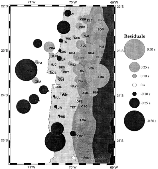
The P-wave station corrections (Fig. 5) show a clear trend On the other hand, a mispicked S arrival time at a station close to the epicentre can result in a stable solution with a from negative values in the west to positive values in the east.
This trend is mainly caused by high velocities within the small RMS, but that actually denotes a significantly mislocated hypocentre even for cases with excellent azimuthal station subducting oceanic plate dipping to the east. Waves from deep
events in the eastern part travelling up-dip along this high- coverage. Since the onset of S phases is often masked or distorted by P-wave coda, mispicking is more likely to occur velocity anomaly on their way to the OBH are faster than
those calculated for the 1-D velocity model, which results in with S phases, and a critical quality control is needed. To reduce the possibility of mispicked S arrival times we rotate negative traveltime residuals. Down-dip ray paths through the
subducting oceanic plate and low near-surface velocities due and integrate the horizontal components before picking. After phase picking, we relocate all events with a consistent-velocity to sediment coverage of the Longitudinal Valley are responsible
for the observed positive station corrections of stations on model and select only those events with a GAP<180° and with at least 10 good P and five good S phases. To check land in the eastern part of the network.
Figure 5. Final P-wave station corrections for the minimum 1-D velocity model. The reference station (COL) is marked by a white star. For further discussion see text.
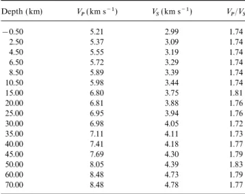
Table 1. P-wave and S-wave velocities and resulting VP/VS ratio of
for data blunders we plot histograms of the residuals sorted
the minimum 1-D velocity model.
by observation weight and eliminate data with exceptional residuals. A final check includes plotting P-arrivals and S–P
Depth ( km) V
P( km s−1) VS( km s−1) VP/VS
arrivals in a Wadati diagram and eliminating phases lying far off the main trend. The final data set for the P- and
S-−0.50 5.21 2.99 1.74
wave inversion consists of 560 events with 12 574 P and 2.50 5.37 3.09 1.74
7429 S phases. 4.50 5.55 3.19 1.74
In general, S phases are included in the location procedure 6.50 5.72 3.29 1.74 by simply assuming a constant VP/VS ratio. By synthetic testing, 8.50 5.89 3.39 1.74
10.50 5.98 3.44 1.74
Maurer & Kradolfer (1996) showed that focal-depth errors
15.00 6.80 3.75 1.81
obtained with a fixed VP/VS ratio are nearly twice as large
20.00 6.81 3.88 1.76
as the errors using P-phases only. The use of an independent
25.00 6.95 3.94 1.76
S-wave velocity yielded the best results. Consequently, we
deter-30.00 6.98 4.05 1.72
mined a minimum 1-D S-wave velocity model by an additional
35.00 7.11 4.11 1.73
series of inversions.
40.00 7.41 4.18 1.77
Four different VP/VS values ranging from 1.6 to 1.9 were 45.00 7.69 4.30 1.79 chosen to construct four initial S-wave velocity models for the 50.00 8.05 4.39 1.83 joint P- and S-wave velocity inversion (Fig. 6). In each case, 60.00 8.48 4.73 1.79 the previously calculated minimum 1-D P-velocity model 70.00 8.48 4.78 1.77
with corresponding station corrections was taken as the initial P-wave velocity model. Equal damping of the P-wave velocities results in unrealistically high P-wave velocities for the shallow
Stability of the minimum 1-D model of the Antofagasta area
layers where no events are located. For this reason, P-wave
velocities for the topmost 15 km were more or less fixed to the To test the stability of the final P- and S-wave minimum 1-D velocity model we performed various tests with randomly and initial values by strong overdamping. Fig. 6 and Table 1 show
the final P- and S-wave velocities and the corresponding VP/VS systematically shifted hypocentres. Shifting the hypocentres randomly in one direction by 10–15 km before introducing ratio for the various initial models. For depths shallower than
15 km, the VP/VS ratio is close to the initial value. VP/VS ratios them into the joint velocity–hypocentral parameter inversion provides a check for possible small bias in the hypocentre diverge below 60 km depth for all models, a phenomenon that
was found to be a result of the low number of events within locations and for the stability of the solution to the coupled problem. If the proposed minimum 1-D velocity model denotes this depth range.
Figure 6. Initial (dashed) and final (solid ) P- and S-wave velocity models. The minimum 1-D P-wave velocity model has been taken for all models as the initial P-wave model. The initial S-wave velocities were calculated using various V
P/VS ratios as noted in the plot. P-wave velocities were fixed for all models to a depth of 15 km because of the poor resolution within these layers. The final VP/VS ratios after the 1-D inversion are displayed on the right. The chosen minimum 1-D P- and S-wave velocity model is marked by the bold line. Velocity values are listed in Table 1.
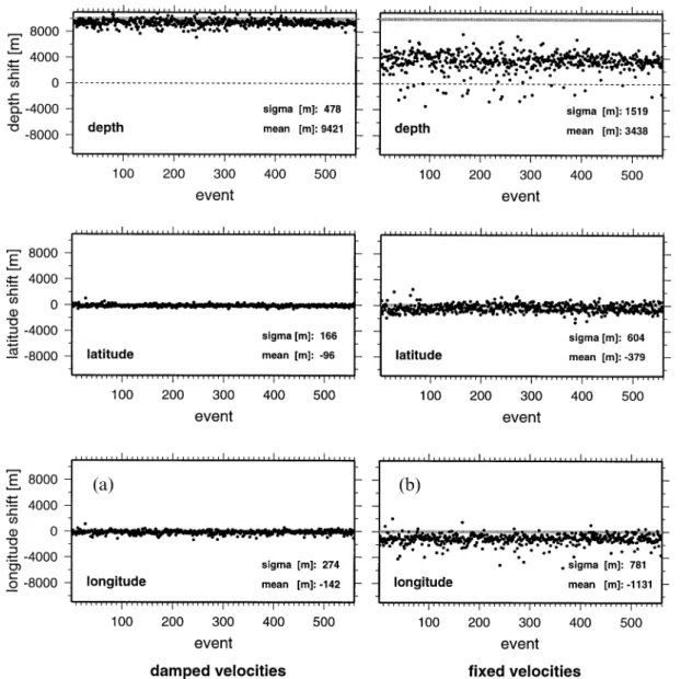
a robust minimum in the solution space, no significant changes The shifting of the hypocentres systematically in one direction, for example focal depth, is a good test for the robustness of in velocity and hypocentre locations are to be expected. Fig. 7
displays the difference in focal depth, latitude, and longitude a minimum 1-D model. After shifting all events to a greater depth by 10 km, two inversions were performed, one with between the original hypocentres (as obtained by independent
P- and S-wave inversion) and the hypocentres that are slightly damped and one with strongly overdamped velocities, the results of which are shown in Figs 8(a) and ( b), respectively. randomly shifted by 10–15 km before being introduced into
the inversion. All events are relocated close to their original Since we solve a coupled hypocentre–velocity problem, the initial bias in the hypocentres may be compensated by adjusting position, demonstrating that the hypocentre locations obtained
by the inversion process are not systematically biased. the velocities, or by relocating the events to their original position, or by a combination of these methods. When reducing the degree of freedom by fixing the velocities during the inversion, the hypocentres are relocated relatively close to their original position (Fig. 8b) except for a shift in depth of 3.4 km. The hypocentres remain in their shifted position (Fig. 8a) when we use regular damping in the inversion. In combination with the previous findings regarding the depth of the hypocentres, the small deviations in latitude and longitude for both test cases (Figs 8a and b) indicate a decoupling of the epicentre problem from the velocity and a strong coupling of the depth/origin-time problem to the velocity for our data set.
Accuracy of hypocentre locations
The relocation of mine blasts or shots provides a good absolute error estimate for hypocentre locations. To provide independent information for such testing, these data were not included in the previous inversion process. The error expected from this approach will be higher than that of earthquakes at greater depth, because for events located close to the surface the waves travel twice through shallow and heterogeneous structures poorly accounted for by the model (Kissling 1988, his Fig. 14). In the CINCA experiment, near-surface velocities are poorly constrained, because most rays travel nearly vertically at shallow depths due to the unfavourable event-depth distribution. Seven blasts in the Mantos Blancos copper mine situated inside the network were relocated using the minimum 1-D model for P- and S-wave velocities with corre-sponding station corrections. The mislocation vectors of the relocated blasts relative to the true mine location are shown in Fig. 9. The diameter of the circle represents the uncertainty of the blasts within the mine. The first relocations (marked by circles in Fig. 9) with the minimum 1-D model result in precise epicentre positions; focal depths, however, show consistently large offsets. This unexpected large deviation in depth could be caused by an inadequate approximation of the local near-surface velocities in the vicinity of the mine. To overcome this problem, we relocate the mine blasts performing a P- and S-wave inversion with all velocities fixed except those of the first two layers, which are regularly damped. The new positions with adjusted near-surface velocities (marked as stars in Fig. 9) show identical results for the epicentres and a more realistic focal depth. Hence, we estimate an absolute error of 1 km in epicentre location and of 2 km in focal depth.
Improvement on hypocentre locations using OBH data
Figure 7. Mislocation of hypocentres randomly shifted by 10 to 15 km before being introduced into the 1-D P+S inversion using the
Apart from the applied velocity model, hypocentre locations
minimum 1-D P+S velocity model. Grey dots denote the systematic
are also sensitive to the azimuthal distribution of stations
shift of the hypocentre locations before introducing them into the
observing the event. Since a significant part of the aftershock
inversion. All hypocentres are relocated to their original position,
series is located offshore, the OBHs are of obvious importance
indicating that no location bias is present. The relative mislocation
in the extension of the seismic network over the seismogenic
error in focal depth is nearly twice that in latitude and longitude, as
Figure 8. (a) Mislocation of hypocentres systematically shifted to greater depth before being introduced into the 1-D P+S inversion using the minimum 1-D P+S velocity model. Damping of the velocities prevents a relocation of the hypocentres to their original positions. (b) As (a), but with fixed velocities. Hypocentres are now relocated close to their original positions. Note the weak influence of the shift in depth on latitude and longitude, indicating the decoupling of epicentre and depth/origin-time determination. Grey dots denote the systematic shift of the hypocentre locations before their introduction into the inversion.
investigate the influence of the OBH data on hypocentre location problem provides an estimate of the interdependence of the resulting hypocentral parameters. For a perfect solution, locations we established a second minimum 1-D model using
only stations on land. An unfavourable distribution of selected the corresponding diagonal element is close to one. Table 3 summarizes the resolution diagonal elements for the selected earthquakes prevented us from resolving the expected strong
variations in the upper crust between the offshore and onshore event and for both locations (with/without OBHs). A strong decrease for the diagonal elements corresponding to longitude areas. Hence, the differences between these two minimum 1-D
velocity models are small. The changes in the hypocentres and focal depth is clearly visible. The first is a response to the lack of stations located to the west of the epicentre when discussed below are therefore mainly due to alterations in the
geometry of the location problem. neglecting the OBHs. The lower resolution in focal depth results from the loss of a station within the focal-depth distance. Differences in hypocentre locations of up to 9 km in focal
depth and 4 km in epicentre are observed when locating the Readings within these distances provide a tighter constraint on the hypocentre location than those with larger offsets offshore events with and without OBHs. To demonstrate that
these mislocations are due to an unfavourable azimuthal (Gomberg et al. 1990). Consequently, the poorer resolution in longitude and focal depth for the location without the OBHs coverage, we computed for each case the resolution matrix for
one event. Fig. 10 shows the azimuthal coverage and Table 2 is expressed in a large difference in focal depth and longitude between the two locations.
lists the hypocentre locations obtained with and without OBH
for this event. Analogous to seismic tomography and other Computing and analysing the resolution matrix for a large set of earthquakes is obviously impractical. RMS values, inversion studies, the resolution matrix for the hypocentre
Figure 10. Azimuth distribution of recorded stations for an offshore event located with and without OBHs. Details of location accuracy can be found in the text and Tables 2 and 3.
Table 2. Statistical parameters for selected events located with and Figure 9. Mislocation in epicentre (top) and depth (bottom) of relocated
without OBHs. Mantos Blancos blasts. The large offset for the events marked by a
circle is due to in inadequate approximation of the near-surface velocities
with OBH without OBH
of the minimum 1-D model. Adjusting the velocities results in a more realistic depth (marked with stars). Using these relocations, the location
latitude 23.5761°S 23.5704°S
error is estimated to 2 km in depth and to 1 km in epicentre.
longitude 70.8156°W 70.7855°W
focal depth 14.64 km 23.14 km
however, are a poor diagnostic tool for judging the quality of
no. of phases (P+S) 34 40
hypocentre solutions. In the test event, we observe a smaller
Pmin 13 km 28 km
RMS value for the location obtained without using OBHs. S
min 28 km 28 km
This is a consequence of the smaller number of stations for GAP 77° 235° this event, which in general results in a lower RMS estimate. RMS 0.24 s 0.17 s Rather than the RMS value or the full resolution matrix, we ALE 1.814 2.166
propose to use the Dirichlet spread function (DSPR) and the DSPR 0.025 0.210
average logarithmic eigenvalue (ALE), which were introduced by Kradolfer (1989). The ALE is based on the eigenvalues of
the hypocentre location problem and qualifies the geometry ALE and DSPR values for all events located with and without OBH data are displayed in Figs 11 and 12, respectively. of an earthquake location problem. For an optimal location
geometry, the ALE is close to zero. The DSPR is based on Nearly identical results are achieved in the onshore area for the two location problems, indicating the weak influence of the L
2 norm of the difference between the resolution matrix
for the problem and an identity matrix (Menke 1984), and OBH data on events located beneath land stations. As expected, large differences exist in the offshore area. As a consequence describes the goodness of resolution or how well the problem
can be solved. For a perfect resolution, the resolution matrix of the unfavourable azimuthal coverage, ALE and DSPR increase rapidly when the OBH data are not included. Without becomes the identity matrix and, consequently, the spread is
zero. In Table 2 the ALE and DSPR values are listed for both the use of OBHs, reliable offshore hypocentre determination is therefore restricted to the region within the land station locations. Both methods give larger values for the hypocentre
location obtained without OBHs, and hence, based on the network. Mislocations in focal depth and epicentre of offshore events without the use of OBHs—or in general for events diagnostic tools (ALE and DSPR), one obtains the correct
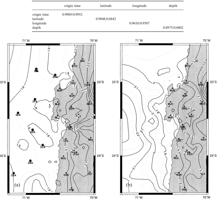
Table 3. Diagonal elements of the resolution matrix located with/without OBH. For further discussion see text.
origin time latitude longitude depth
origin time 0.9989/0.9952
latitude 0.9048/0.6842
longitude 0.9610/0.9507
depth 0.8975/0.6802
Figure 11. (a) Contour lines of ALE values for events located with OBHs. The contour interval is 0.05. ( b) As (a), but now all events are located without OBH data. Higher values offshore indicate the poorer geometry of the location problem because of the neglect of the important OBH phases.
focal depth and 4 km in epicentre, which is more than three areas can be identified: one located at the southern tip of the Mejillones Peninsula and one offshore towards the centre times the estimated mislocation vector.
of the rupture zone. These two locations coincide with the locations of the two main sources, which released 74 per cent
D I S T R I B U T I O N OF T H E A N T OFA G A S TA
of the total seismic moment (Delouis et al. 1997). Besides the
AF T E R SH O C K S
aftershock activity, a small amount of background seismicity is observed.
Fig. 13 shows the final hypocentre locations of all 560
well-locatable events used in the P- and S-wave inversion. A The longitudinal depth section reveals a sharp upper boundary of the Wadati Benioff zone (WBZ), which dips at latitudinal depth section is plotted on the right side of the
central figure, and a longitudinal depth section is plotted along an average angle of 19°–20° to a depth of 50 km (Fig. 13). This dip corresponds to the estimated dip of the fault-plane the bottom. In the lower right corner, the minimum 1-D
models for P- and S-wave velocities are displayed. solution of the main shock (Delouis et al. 1997). Towards the trench, seismicity is low (Fig. 2) and no reliable hypocentres The majority of epicentres are concentrated within the
rupture area of the main shock as determined by Delouis could be determined for these events outside the network. Below 50 km depth and east of 70°W the pattern of seismicity et al. (1997). It seems that within this rupture area two
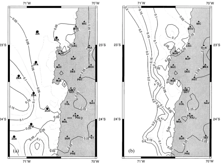
sub-Figure 12. (a) Contour lines of Dirichlet-Spread values for events located with OBHs. The contour interval is 0.025. ( b) As (a), but now all events are located without OBH data. The higher values offshore indicate lower resolution. Reliable hypocentres are now limited to a narrow stretch along the coast.
changes remarkably, as observed by other workers (Comte offsets (Armijo & Thiele 1990; Delouis et al. 1998). Preliminary focal mechanism solutions of five events of the cluster show et al. 1994; Delouis et al. 1996). The sharp upper boundary
disappears and the depth distribution becomes irregular. This two strike-slip and three mainly normal fault solutions. Since this area is within the rupture zone of the Antofagasta main change probably indicates the maximum depth of the rupture
zone and coincides with the transition from a compressional shock and the clustering of the events happens in space and time, it is likely that the observed crustal activity was triggered stress regime to a more tensional one (Comte et al. 1994;
Comte & Suarez 1995; Delouis et al. 1996). by the main shock, but further study is needed to confirm a possible relation to the Atacama Fault System. No events have During our observation period crustal seismicity was at a
very low level, although the area under study shows recent been detected at shallow crustal levels, which may be due to the high noise level generated by the aftershock activity. fault activity, mainly of extensional character (Armijo & Thiele
1990; Delouis et al. 1998). A cluster of six events was detected On the other hand, no shallow seismicity has been reported by other workers (Comte et al. 1994; Delouis et al. 1996), in in the lower crust at a depth of 21 km, clearly separated from
the main activity along the Wadati Benioff zone (Fig. 13). contrast to the fault activity observed at the surface (Armijo & Thiele 1990; Delouis et al. 1998).
Excellent azimuthal coverage leads to an estimated location error of only 2 km in focal depth for these events. They occurred within one day and show a magnitude of up to 4.0
M A X I M U M A N D M I N I M U M D E P T H O F
as determined by the local network. The location of the
epi-T H E C O U P L E D S E I S M O G E N I C Z O N E
centres suggests a possible relation of these events with the
Atacama Fault System, a major zone of deformation that The extent of the seismogenic zone has been studied by analysing either the distribution of focal mechanisms of the stretches nearly parallel to the coastline at an offset of 30–50 km
for about 1100 km (Armijo & Thiele 1990). Deformation normal seismicity (e.g. Comte et al. 1994; Delouis et al. 1996) or the aftershock distribution of a great underthrust event observed along the Atacama Fault System is characterized
by vertical uplift and subsidence related to normal faulting. within the seismogenic zone (Tichelaar & Ruff 1993). Both approaches complement each other and are needed to define Strike-slip components are also observed but with moderate
Figure 13. Accurate hypocentres as determined by an independent P+S inversion using a combined on-/offshore network. Vertical depth sections along latitude and longitude are shown at the bottom and right side, respectively. The minimum 1-D velocity model for P- and S-waves is displayed on the lower right. The area marked by the dashed line denotes the rupture area of the Antofagasta main shock, after Delouis et al. (1997 ).
clearly the extent of the seismogenic zone within a subducting Since our analysis of the seismogenic zone is based on the high-precision location of the aftershock series of a great plate. In general, the determination of the maximum and
mini-mum depths of the seismogenic zone has been based on underthrust event, we are able to give reliable estimates for both the minimum and maximum depths of the seismogenic detailed focal mechanism analysis. Several studies in northern
Chile aimed to define the extent of the coupled plate interface. zone. In order to exclude earthquakes located within the subducting oceanic plate from the study, we select only the Comte et al. (1994) used focal mechanisms of locally recorded
earthquakes and found a maximum depth of shallow-dipping shallowest event within a specified bin width. Fig. 14 displays thrust events of 47 km in the Antofagasta area. Recently,
Delouis et al. (1996) performed a simultaneous determination of orientation and shape of the local stress tensor and of individual focal mechanisms using locally recorded earth-quakes within the Antofagasta region, and found the lower limit of the coupled plate interface at a depth of 50 km. Tichelaar & Ruff (1991) used focal mechanisms from teleseismically recorded aftershocks of magnitudes greater than 6 for the central and northern part of the Chilean subduction zone. Their results of a maximum depth of 46–48 km for northern Chile are poorly constrained because no large earthquake ruptured this area between 1877 and 1995. None of these earlier studies regarding the extent of the seismogenic zone can provide a reliable value for the minimum depth of the coupled plate interface. The use of teleseismic events at shallow depths in subduction zones relies strongly on the knowledge of bathymetry and/or properties of the uppermost sedimentary
layers (Pacheco et al. 1993; Wiens 1989). On the other hand, Figure 14. Depth distribution of events belonging to the aftershock local networks used by Comte et al. (1994) and Delouis et al. series. The data have been binned using only the shallowest events in (1996) failed to determine accurate depths for offshore events each bin. The distribution could be fitted well by a double Gaussian
distribution (see text for more details).
the focal depth distributions of these events. Our data have a chlorite, which are more frictionally unstable (Hyndman & Wang 1995). Although sediment coverage is low in the trench good fit to a double Gaussian distribution with depth, although
the second maximum is not very dominant. Following Pacheco axis (Hinz et al. 1995), our results may suggest that the dehydration of stable clays controls the upper limit of the et al. (1993), we define the maximum and minimum depths
of the seismogenic zone by the 95th and the 5th percentile, seismogenic zone. respectively. This approach accounts for uncertainties in depth
distribution resulting from location errors and from
incom-C O N incom-C L U S I O N S
pleteness due to the restricted observation period. With this
approach we find the maximum depth of the seismogenic zone Applying the concept of the minimum 1-D model results in uniformly precise and reliable hypocentre locations within the at a depth of 46 km, which fits well in the range found by
Tichelaar & Ruff (1991), Comte & Suarez (1995) and Delouis network that monitored aftershocks of the 1995 Antofagasta earthquake. Neglecting the individual station elevation in the et al. (1996), and the minimum depth at 20 km depth.
Numerical modelling of the temperature field of the coupling inversion process yields station corrections that depend both on near-surface heterogeneities beneath the station and on interface supports the concept that a critical temperature may
play a key role in controlling the extent of the seismogenic station elevation. By relocating mine blasts, we calculate a mislocation vector of 1 km for the epicentre and 2 km for zone. A critical temperature of 100–150°C was found at the
upper boundary (Hyndman & Wang 1995) and of 250°C or the focal depth. This mislocation estimate for blasts denotes an upper boundary for deeper events (Kissling 1988). The 400–550°C at the lower boundary, depending on the
distri-bution of shear stress at the coupling interface (Tichelaar & relatively low mislocation values and the results of stability tests with randomly and systematically shifted hypocentres Ruff 1993; Hyndman & Wang 1995). Models of the temperature
field in the forearc region of the Antofagasta area (Springer demonstrate that the minimum 1-D model concept is capable of accurate hypocentre location even in areas of predominantly 1997) show a temperature of 200–250°C for a depth of 46 km,
corresponding to the maximum depth of the seismogenic zone. 2-D structure. Parameters essential for hypocentre accuracy are a suitable distribution of recording stations and the use of S-wave Tichelaar & Ruff (1993) pointed out that the distribution of
shear stress along the coupling interface is an important arrival times. Reliable hypocentres may only be obtained for events with an azimuthal gap of recording stations of less than parameter for the critical temperature at the lower boundary.
Assuming a constant coefficient of friction, they found two 180°, as documented in detail by analysis of the resolution parameters ALE and DSPR introduced by Kradolfer (1989). critical temperatures of 400°C and 550 °C. Assuming constant
stress with depth, however, they found a single critical temper- Hence, without the OBHs, reliable hypocentre determination is restricted to the region within the land-station network. ature of 250°C. To explain the low values of heat flow observed
in the Antofagasta forearc region, Springer (1997) used a con- Precise location of the aftershock series of the large Antofagasta underthrust event (1995 July 30; M
w=8.0) pro-stant shear stress for the thermal modelling, thereby explaining
the low critical temperature found at the lower boundary of vides a detailed image of the seismogenic zone, where the coupling between the subducting Nazca plate and the overlying the seismogenic zone.
Byrne et al. (1988) recognized that in most subduction zones South American plate takes place. This seismogenic zone dips at an angle of about 19°–20°, and we determined a depth of earthquakes do not extend up-dip along the plate interface all
the way to the trench axis or deformation front. They argued 46 km for its lower limit. This agrees well with previously published results inferred from fault plane solutions of locally that the existence of this aseismic zone is caused by stable
slip properties of the unconsolidated and semiconsolidated and teleseismically recorded earthquakes. Since the network incorporated the use of OBHs, we had good control over sediment in that zone. At greater depth the sediment becomes
more consolidated and de-watered and comes into contact events located offshore and were able to locate the upper limit of the seismogenic zone at a depth of 20 km. This value is with harder rocks of the overlying plate. Here the slip behaviour
changes to unstable stick-slip sliding accommodated seismically constrained by two other observations: von Huene et al. (1998) proposed the existence of a detachment zone above as episodic slip in large earthquakes. Sediments are essentially
lacking in the trench axis off northern Chile (Hinz et al. 1995), the seismogenic zone to decouple the compressional tectonic regime along the plate interface and the tensional regime at however, and the subduction zone along northern Chile has
been characterized as erosional type (von Huene & Scholl the surface. Numerical modelling of the temperature field of the Antofagasta forearc region (Springer 1997) suggests that 1991). A detachment zone which decouples the converging
upper and lower plates and which is only effective seawards dehydration of clays to illites and chlorites, which are more frictionally unstable, may control the upper limit of the seismo-of the seismogenic zone (von Huene et al. 1998) may be
responsible for the observed lack of stronger seismic events at genic zone, although sediment coverage is low in the trench axis.
shallow depths. Such a detachment zone is required to explain the existence of a compressional tectonic regime along the plate interface and the extensional tectonic regime observed
A C K N O W L E D G M E N T S
at the surface of the seaward slope of the overlying plate
(von Huene et al. 1998). Events associated with the detachment We wish to thank the SFB 267, the master, crew and scientists of the RV Sonne during legs 2 and 3 of the cruise SO104, and itself are probably too weak to be detected by the network
and are concealed by the high number of aftershocks. everyone who maintained the stations and pre-processed the data in the field. A. Rietbrock helped us with all questions Thermal modelling of the Antofagasta forearc region gives
a temperature of 120–150°C for the upper limit of the seismo- regarding the software. M. Sobiesak and R. Patzig helped us with the picking of first arrivals of the large data genic zone. Within the range of uncertainty, this corresponds
Kissling, E., 1988. Geotomography with local earthquakes, Rev.
F. Graeber. Most of the plots were generated using the Generic
Geophys., 26, 659–698.
Mapping Tool of Wessel & Smith (1995). The CINCA project
Kissling, E. & Lahr, J.C., 1991. Tomographic image of the Pacific Slab
is a co-operative research project by the Bundesanstalt fu¨r
under southern Alaska, Eclogae geol. Helv., 84/2, 297–315.
Geowissenschaften und Rohstoffe Hannover, the SFB 267,
Kissling, E., Ellsworth, W.L., Eberhart-Phillips, D. & Kradolfer, U.,
GEOMAR Kiel, GFZ Potsdam, the Catholic University of
1994. Initial reference models in local earthquake tomography,
the North, Antofagasta, and the University of Chile, Santiago. J. geophys. Res., 99, 19 635–19 646.
The CINCA project is funded by the German Federal Ministry Kissling, E., Kradolfer, U. & Maurer, H., 1995a. V EL EST User’s Guide for Education, Science, Research and Technology (BMBF) – Short Introduction, Institute of geophysics and Swiss seismological
under grant 03G0104. We thank D. Comte, G. Bock, and an service, ETH, Zurich.
Kissling, E., Solarino, S. & Cattaneo, M., 1995b. Improved seismic
anonymous referee for their careful and critical reviews.
velocity reference model from local earthquake data in Northwestern Italy, T erra Nova, 7, 528–534.
Kradolfer, U., 1989. Seismische Tomographie in der Schweiz mittels
RE F E R E N C E S lokaler Erdbeben, Phd thesis, ETH, Zu¨rich.
Maurer, H. & Kradolfer, U., 1996. Hypocentral parameters and Armijo, R. & Thiele, R., 1990. Active faulting in northern Chile, ramp
velocity estimation in the western Swiss alps by simultaneous stacking and lateral decoupling along a subduction plate boundary?,
inversion of P- and S-wave data, Bull. seism. Soc. Am., 86, 32–42. Earth planet. Sci. L ett., 98, 40–61.
Menke, W., 1984. Geophysical Data Analysis: Discrete Inverse T heory, Asch, G., Wylegalla, K., Graeber, F., Haberland, Ch., Rudloff, A.,
Academic Press, San Diego. Giese, P. & Wigger, P., 1994. PISCO 94, Proyecto de Investigacion
Pacheco, J.F., Sykes, L.R. & Scholz, C.H., 1993. Nature of seismic Sismologica de la Cordillera Occidental—Teil 1, Erdbebenregistrierung,
coupling along simple plate boundaries of the subduction type, T erra Nova, 2/94, 14.
J. geophys. Res., 98, 14 133–14 159. Asch, G., Bock, G., Graeber, F., Haberland, Ch., Hellweg, M., Kind, R.,
Rietbrock, A. & Scherbaum, F., 1998. The GIANT analysis system Rudloff, A. & Wylegalla, K., 1995. Passive Seismologie im Rahmen
(graphical interactive aftershock network toolbox), Seism. Res. L ett., von PISCO∞94, Report of the SFB 267 ‘Deformation processes in the
69, 40–45. Andes’, pp. 619–667, Berlin.
Ruff, L., 1996. Large earthquakes in subduction zones: segment Byrne, D.E., Davis, D.M. & Sykes, L.R., 1988. Loci and maximum
interaction and recurrence time, in Subduction: T op to Bottom, size of the thrust earthquakes and the mechanics of the shallow
pp. 91–105, eds Bebout, G.E., Scholl, D.W., Kirby, S.H. & Platt, P., region of subduction zones, T ectonics, 7, 833–857.
Geophysical Monograph 96, AGU. Comte, D. & Suarez, G., 1995. Stress distribution and geometry of the
Ruff, L. & Tichelaar, B., 1996. What controls the seismogenic plate subducting Nazca plate in northern Chile using teleseismically
interface in subduction zones, in Subduction: T op to Bottom, recorded earthquakes, Geophys. J. Int., 122, 419–440.
pp. 105–1013, eds Bebout, G.E., Scholl, D.W., Kirby, S.H. & Platt, P., Comte, D., Pardo, M., Dorbath, L., Dorbath, C., Haessler, H., Rivera, L.,
Geophysical Monograph 96, AGU. Cisterna, A. & Ponce, L., 1994. Determination of seimogenic
Scheuber, E., Bogdanic, T., Jensen, A. & Reutter, K.-J., 1994. Tectonic interplate contact zone and crustal seismicity around Antofagasta,
development of the North Chilean Andes in relation to plate northern Chile using local data, Geophys. J. Int., 116, 553–561. convergence and magmatism since the Jurassic, in T ectonics of the Crosson, R.S., 1976. Crustal structure modeling of earthquake data, 1, Southern Central Andes, pp. 121–139, eds Reutter, K.-J., Scheuber, E.
Simultaneous least squares estimation of hypocenter and velocity & Wigger, P.-J., Springer Verlag, Berlin.
parameters, J. geophys. Res., 81, 3036–3046. Solarino, S., Kissling, E., Cattaneo, M. & Eva, C., 1997. Local Delouis, B., Cisternas, A., Dorbath, L., Rivera, L. & Kausel, E., 1996. earthquake tomography of the southern part of the Ivrea body,
The Andean subduction zone between 22 and 25° S (northern Chile): North-Western Italy, Eclogae geol. Helv., 90, 357–364.
precise geometry and state of stress, T ectonophysics, 259, 81–100. Springer, M., 1997. Die Oberfla¨chenwa¨rmefludichte-Verteilung in den Delouis, B., Monfret, T., Dorbath, L., Pardo, M., Rivera, L., Comte, D., zentralen Anden und daraus abgeleitete Temperaturmodelle der
Haessler, H., Caminade, J.P., Ponce, L., Kausel, E. & Cisternas, A., Lithospha¨re, PhD thesis, FU-Berlin.
1997. The Mw=8.0 Antofagasta (northern Chile) earthquake of Thurber, C.H., 1992. Hypocenter-velocity structure coupling in 30 July 1995: a precursor to the end of the large 1877 gap, Bull. local earthquake tomography, Phys. Earth planet. Inter., 75,
seism. Soc. Am., 87, 427–445. 55–62.
Delouis, B., Philip, H., Dorbath, L. & Cisternas, A., 1998. Recent Tichelaar, B. & Ruff, L., 1991. Seismic coupling along the Chilean crustal deformation in the Antofagasta region (northern Chile) and subduction zone, J. geophys. Res., 96, 11 997–12 022.
the subduction process, Geophys. J. Int., 132, 302–338. Tichelaar, B. & Ruff, L., 1993. Depth of seismic coupling along Eberhart-Phillips, D. & Michael, A.J., 1993. Three-dimensional velocity subduction zones, J. geophys. Res., 98, 2017–2037.
structure, seismicity, and fault structure in the Parkfield region, von Huene, R. & Scholl, D.W., 1991. Observations at convergent central California, J. geophys. Res., 98, 737–758. margins concerning sediment subduction, subduction erosion and Gomberg, J.S., Shedlock, K.M. & Roecker, S.W., 1990. The effect of the growth of continental crust, Rev. Geophys., 29, 279–316.
S-wave arrival times on the accuracy of the hypocenter estimation, von Huene, R., Weinrebe, W. & Heeren, F., 1999. Subduction erosion Bull. seism. Soc. Am., 80, 1605–1628. along the north Chilean margin, J. Geodyn., 27, 345–358. Graeber, F., 1997. Seismische Geschwindigkeiten und Hypozentren in den Wessel, P. & Smith, W.H.F., 1995. New version of the Generic
su¨dlichen zentralen Anden aus der simultanen Inversion von Laufzeit- Mapping Tool released, EOS, T rans. Am. geophys. Un., 76, 329. daten des seismologischen Experiments PISCO’94 in Nordchile, Wiens, D., 1989. Bathymetric effects on body waveforms from shallow Scientific T echnical Report ST R97/17, GeoForschungszentrum, subduction earthquakes and application to seismic processes in the
Potsdam. Kuril Trench, J. geophys. Res., 98, 2955–2972.
Hinz, K. et al., 1995. Crustal investigations off- and onshore Nazca/ Wigger, P.J., Schmitz, M., Araneda, M., Asc, G.H., Baldzuhn, P., Central Andes, CINCA, Sonne Cruise 104, Leg 1, 22.07.–24.08. 1995, Giese, P., Heinsohn, W.-D., Martinez, E., Ricaldi, E., Ro¨wer, P. Bundesanstalt fu¨r Geowissenschaften und Rohstoffe, Hannover, & Viramonte, J., 1994. Variation in the crustal structure of the Archiv–Nr. BGR 113.998, Tagebuch–Nr. 12. 192/95. Southern Central Andes deduced from seismic refraction investi-Hyndman, R.D. & Wang, K., 1995. The rupture zone of Cascadia gation, in T ectonics of the Southern Central Andes, pp. 23–48, great earthquakes from current deformation and thermal regime, eds Reutter, K.-J., Scheuber, E. & Wigger, P.-J., Springer Verlag,
Berlin. J. geophys. Res., 100, 22 133–22 154.