HAL Id: hal-01904323
https://hal.archives-ouvertes.fr/hal-01904323
Submitted on 29 Oct 2018
HAL is a multi-disciplinary open access
archive for the deposit and dissemination of
sci-entific research documents, whether they are
pub-lished or not. The documents may come from
teaching and research institutions in France or
abroad, or from public or private research centers.
L’archive ouverte pluridisciplinaire HAL, est
destinée au dépôt et à la diffusion de documents
scientifiques de niveau recherche, publiés ou non,
émanant des établissements d’enseignement et de
recherche français ou étrangers, des laboratoires
publics ou privés.
Finite size effects on crack front pinning at
heterogeneous planar interfaces: Experimental, finite
elements and perturbation approaches
Sylvain Patinet, Lina Alzate, Etienne Barthel, Davy Dalmas, Damien
Vandembroucq, Veronique Lazarus
To cite this version:
Sylvain Patinet, Lina Alzate, Etienne Barthel, Davy Dalmas, Damien Vandembroucq, et al.. Finite
size effects on crack front pinning at heterogeneous planar interfaces: Experimental, finite elements
and perturbation approaches. Journal of the Mechanics and Physics of Solids, Elsevier, 2013, 61 (2),
pp.311-324. �10.1016/j.jmps.2012.10.012�. �hal-01904323�
Finite size effects on crack front pinning at heterogeneous planar interfaces:
experimental, finite elements and perturbation approaches
S. Patineta, L. Alzateb, E. Barthelb, D. Dalmasb, D. Vandembroucqa, V. Lazarusc
aLaboratoire PMMH, UMR 7636 CNRS/ESPCI/P6/P7, 10 rue Vauquelin, 75231 Paris cedex 05, France
bSurface du verre et interfaces, Unit´e Mixte CNRS / Saint-Gobain UMR 125 (SVI), 39 quai Lucien Lefranc, 93300 Aubervilliers, France cUPMC Univ Paris 6, Univ Paris-Sud, CNRS, UMR 7608, Lab FAST, Bat 502, Campus Univ, F-91405 Orsay, France
Abstract
Understanding the role played by the microstructure of materials on their macroscopic failure properties is an im-portant challenge in solid mechanics. Indeed, when a crack propagates at a heterogeneous brittle interface, the front is trapped by tougher regions and deforms. This pinning induces non-linearities in the crack propagation problem, even within Linear Elastic Fracture Mechanics theory, and modifies the overall failure properties of the material. For example crack front pinning by tougher places could increase the fracture resistance of multilayer structures, with in-teresting technological applications. Analytical perturbation approaches, based on Bueckner-Rice elastic line models, focus on the crack front perturbations, hence allow for a description of these phenomena. Here, they are applied to experiments investigating the propagation of a purely interfacial crack in a simple toughness pattern: a single defect strip surrounded by homogeneous interface. We show that by taking into account the finite size of the body, quanti-tative agreement with experimental and finite elements results is achieved. In particular this method allows to predict the toughness contrast, i.e. the toughness difference between the single defect strip and its homogeneous surrounding medium. This opens the way to a more accurate use of the perturbation method to study more disordered hetero-geneous materials, where the finite elements method is less adequate. From our results, we also propose a simple method to determine the adhesion energy of tough interfaces by measuring the crack front deformation induced by known interface patterns.
Keywords: Interfacial brittle fracture, Toughening, Crack pinning, Finite element method, Perturbation approach
1. Introduction
Predicting the threshold for crack propagation is a key issue in material science: it determines the design quality of structures and their durability for a wide range of systems ranging from bulk materials to thin films. In particular it was shown that one of the most efficient mechanisms to increase effective toughness is crack pinning by material heterogeneities (Bower and Ortiz, 1991). For example the macroscopic effective toughness of a material can be in-creased very significantly by the dispersion of hard particles in the matrix (Mower and Argon, 1995). Another system that takes advantage of crack pinning consists of patterned interfaces presenting heterogeneous toughness landscapes. Their technological interest lies in the development of multi-layer materials with high mechanical stability. A promis-ing method to develop new materials consists in designpromis-ing optimal heterogeneous interfaces with high toughness while maintaining their functional features.
Heterogeneities affect the effective toughness by interfering with crack propagation, deflecting crack fronts and crack surfaces. However, it is difficult to predict the effect of heterogeneities quantitatively and experimental inves-tigation of this toughening mechanism raises several difficulties. For example it is not easy to create well controlled heterogeneity distributions and to observe crack propagation in situ. Also, due to crack deflection, the problem is often three-dimensional and theoretical or numerical developments become quite complex.
In the literature, most of the experimental investigations on crack pinning in heterogeneous materials were statisti-cal approaches and studied post-mortem fracture surfaces (Bouchaud, 1997; Santucci et al., 2007; Ponson et al., 2007; Dalmas et al., 2008; Bonamy, 2009). Experiments with direct visualization of the crack front in situ during propaga-tion are very unfrequent. For example, with an original experimental setup, Schmittbuhl and Måløy (1997) were able
to observe the crack front morphology during propagation along a disordered heterogeneous interface. This setup has been widely used to obtain statistical information on crack front roughness (Delaplace et al., 1999; Santucci et al., 2010) and stochastic dynamics of propagation (Måløy and Schmittbuhl, 2001; Tallakstad et al., 2011). However quan-titative predictions seem out of reach, mainly because of the presence of shear on the crack front during loading and the ill-controlled nature of the heterogeneities. Recently, Chopin et al. (2011) proposed a new experimental approach with better controlled heterogeneities, but the setup also suffers from mode mixity. In the experiments of Mower and Argon (1995), the front is trapped by second-phase particles introduced in a brittle epoxy. The front shape becomes complicated since it can not penetrate in the particles, and these experiments are difficult to model analytically.
Here, we report on a study of crack propagation measured along a well controlled patterned interface in a classical Double Cantilever Beam (DCB) geometry. The crack propagates at the weakest interface in a stack of thin films deposited on glass, allowing direct visualization of the crack front. This weakest interface is not homogeneous how-ever: a defect strip with a different interfacial toughness lies at the center of the sample. Several values of toughness contrast have been investigated and we have monitored the interaction of the interface crack with these defects. The interface cracks are either trapped or attracted by the defect depending on the sign of the toughness contrast between the defect strip and its homogeneous surrounding medium. This setup (Barthel et al., 2005; Dalmas et al., 2009) has several advantages: 1) the crack is loaded in pure tensile mode (mode I); 2) the crack propagation is purely interfacial (without deflexion out of the plane of the interface); 3) the toughness contrast can be tuned to keep the deformations of the crack front small.
In the framework of Linear Elastic Fracture Mechanics, propagation criteria are based on the comparison of the Energy Release Rate (ERR) and adhesion energy (Griffith, 1921) – or equivalently of mode I stress intensity factor (SIF) and toughness (Irwin, 1957). The ERR is derived from an elastic analysis, and depends on loading, elastic response of the solid and geometry of both body and crack. Perturbation methods were initiated by Rice (1985), based on Bueckner (1987) weight-function theory, and specifically used by Gao and Rice (1989) to study the morphology of cracks trapped in heterogeneous interfaces. They provide analytical predictions for the variation of the ERR when the crack front is slightly perturbed and effectively describe the crack front as an elastic line. However, the first order formula proposed by Rice (1985) for a half-plane crack in an infinite media does not take into account any finite size effect. In the case of the present measurements, they may provide erroneous predictions for large enough crack front perturbations (deformation or wavelength) in comparison with sample sizes. However several improvements of this formula have been proposed to take into account the finite size of the crack (Gao and Rice, 1987; Gao, 1988; Leblond et al., 1996; Lazarus and Leblond, 2002; Lazarus, 2011), the finite thickness of the body (Legrand et al., 2011) and even the interaction between two cracks (Pindra et al., 2010).
Our aim here is to assess the use of analytical perturbation theories to model crack propagation in heterogeneous interfaces. To evaluate the merits of these models, we need a reference solution which would provide an exact modeling of the data. In the case of the mildly distorted crack fronts proposed here, Finite Element (FE) simulations can be used to determine the local values of the ERR. In addition, with FE simulations, we can accurately take into account the exact geometry of the sample, including the shape of the crack front which is determined experimentally. The experimental method is presented first with some details concerning the synthesis of the samples and the cleavage tests (section 2). From the measured crack front deformations and loadings, the ERR pattern is then de-termined by numerical and theoretical methods. The ERR along the crack front is quantitatively calculated through detailed three-dimensional FE analysis (section 3). Analytical perturbation methods are presented in section 4 and we show how the local ERR contrast can be inferred. Then FE and analytical methods are applied to the different samples and their results compared in section 5. In particular, it is shown that the ERR contrasts calculated by the two approaches are in good agreement if the finite size of the plate is duly taken into account in the analytical perturbation models (Legrand et al., 2011), in contrast to Rice (1985)’s model, which is conventionally used for this type of ge-ometry although it can apply only to infinite half-spaces. We finally discuss the crack propagation criterion and show how these results can be used to give quantitative estimates of local adhesion energy values for textured interfaces in section 6.
2. Experiments
2.1. Synthesis of samples
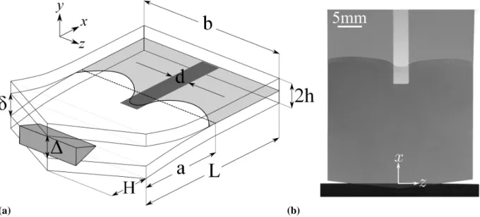
To control and visualize the propagation of a purely interfacial crack along a patterned interface we start from thin film multi-layers deposited by magnetron sputtering (Barthel et al., 2005) on rectangular glass substrates (thickness h = 700 µm, width b, length L). Schematically, a typical sample is glass/silver/top layer (see Fig. 1).
(a)
(b) (c) (d)
Figure 1: (a) Schematics of a patterned multilayer deposited on glass exemplified for the HC-b30 sample. (b), (c) and (d): the multi-layers are reinforced by a glass backing prior to cleavage test for the HC-b30, MC-b40 (MC-b50) and LC-b40 samples respectively (see text for details). The plane of fracture is shown in red.
Patterning of the interface is achieved by inserting a mask close to the sample during deposition of the silver layer. The mask is rectangular (width d) and extends over about half the sample length. The other layers comprising the sample are deposited without mask and are homogeneous. The area covered by the mask induces a zone with different adhesion, i.e. different toughness , which we call the defect strip.
Three types of interfaces are studied, with respectively low toughness contrast (LC), medium contrast (MC) and high contrast (HC). In LC-b40, the defect strip is an organic layer which is directly deposited on glass, inducing lower adhesion. For MC-b40 and MC-b50, the silver layer is deposited on an Si3N4sublayer. The toughness contrast
originates from the difference between Ag/Si3N4and Si3N4/Si3N4adhesion. In HC-b40 the silver layer was deposited
directly on the glass substrate, increasing the toughness contrast due to lower adhesion on glass. The sample nature and dimensions are summarized in Tab. 1, ranked from the lowest to the highest adhesion.
Sample Stack b (mm) L (mm) d (mm) H (mm) Homog. Interf. Defect strip
LC-b40 Gl./Org/Ag/Si3N4 38 64 2.82 3 Glass/Ag Glass/Organic
MC-b40 Gl./Si3N4/Ag/Si3N4 40 65 3.2 3 Si3N4/Ag Si3N4/Si3N4
MC-b50 Gl./Si3N4/Ag/Si3N4 49 82.5 3.87 2.5 Si3N4/Ag Si3N4/Si3N4
HC-b30 Gl./Ag/Si3N4 29.5 36.5 3.2 1.5 Glass/Ag Glass/Si3N4
Table 1: Nature and dimensions of the patterned samples. For each stack the patterned layer is shown in bold. Underlayer thicknesses vary between 10 and 50 nm.
2.2. Cleavage test
To propagate a crack in the multilayer, we use cleavage under ambient conditions: a glass backing of thickness 700 µm is glued on top of the multilayer with an epoxy glue (Barthel et al., 2005; Dalmas et al., 2009), resulting in a glass/multilayer/glass sandwich. This sandwich is amenable to opening in a DCB setup. The test is carried out by progressive opening of the two glass arms by the gradual introduction of a wedge between the two plates (Fig. 2a). The positioning of the wedge is controlled by an electric jack for precise control of the opening of the two glass
plates. With this method, cleavage is displacement controlled and the propagation of the crack is stable: the crack length increases in a controlled way. The propagation of the crack front is performed in a quasi-static manner, i.e. further increment of the opening is applied only after complete arrest of the crack front.
a
2h
(a) (b)
Figure 2: (a) Schematic of cleavage test on a double cantilever beam. The opening of the crack δ is imposed by the wedge in order to control the average length of the crack a. (b) Top view sample photography during the cleavage test HC-b30. Thanks to transparency of the glass, interfacial crack is observed. The deformation of the crack comes from the difference of adhesion energies between the silver interface and the defect strip.
The specimen is semi-transparent and we directly observe the crack front propagation during opening. In order to record the data, two high magnifications cameras are used. The first camera monitors the displacement of the glass arms δ, which is measured at the corners of the crack surfaces (see Fig. 2a). The second camera records the crack front shape a(z) (see Fig. 2b). Its position a(z) is measured from the line parallel to z passing through the external corners of the crack surfaces.
Once the wedge penetrates between the two plates, crack propagation takes place at the weakest interface of the multilayer. In order to identify this interface X-Ray photoelectron spectroscopy is used on both fracture surfaces. In these samples, purely interfacial fractures have always been found. As indicated in Fig. 1, the crack takes place at one of the silver layer interfaces for all the configurations. This observation is consistent with the weak adhesion of silver layers and the perfectly interfacial crack path demonstrated earlier (Barthel et al., 2005). As the crack propagates in a patterned interface, two fracture interfaces can be defined, one involving the silver layer and the other one in the defect strip (see Tab. 1).
The evolution of the crack front morphologies (only for equilibrium positions) during cleavage tests is shown in Fig. 3 in the case of sample HC-b30. In the first regime, the propagation takes place at the homogeneous silver interface. The crack front propagates with the overall curved shape which is characteristic of homogeneous interfaces for finite width samples (Sec. 3.3). This simple curved shape is preserved until the crack comes into contact with the defect strip, where deformation of the crack front begins: it is held back by the defect strip and curves into the outer region. After this transient regime, stationary propagation is recovered: in this third regime, where the crack propagates in the patterned area of the interface, the overall curvature of the crack front is now decorated by an additional modulation: the front lags behind in the high adhesion defect strip.
The crack front positions a(z) and the loadings δ, with the sample geometric dimensions and the elastic constants of the glass (E,ν), serve as input parameters to model the cleavage tests in the next sections by two different ways. We compute the ERR landscape along the crack front first by FE numerical calculations (Sec. 3), second, by theoretical perturbation approaches (Sec. 4) and compare the results (Sec. 5).
-10 0 10 z (mm) 10 15 20 25 30 x (mm) I II III
Figure 3: Evolution of the equilibrium shape of the measured crack front for the HC-b30 sample. The three suc-cessive regimes of propagation are distinguished. I: Stationary propagation along the silver homogeneous interface (wide dashed black lines); II: transient deformation of the front when entering the defect strip (red dotted lines); III: stationary propagation of the deformed front in the defect strip (continuous blue lines).
3. ERR obtained numerically by Finite Elements
FE calculations are performed with the aim to analyze the validity of the analytical perturbation approaches pro-posed in this paper (Sec. 4.2). To directly model the whole experimental pinning cleavage tests and obtain a reference solution of the global and local ERRs, we needed to take into account the whole geometry of the problem, includ-ing specimen geometry and the crack morphology (Sec. 3.1). This is the major part of the present FE calculations (Sec. 3.2). Besides, we also consider the case of an homogeneous interface (Sec. 3.3). Even in this case, due to the finite width of the specimen, the front shapes are not straight and are derived here by FE calculations. They are used as reference unperturbed crack geometry for the perturbation methods.
3.1. Simulation method
To calculate the local ERR distribution, the static elasticity problem is resolved by FE for each equilibrium po-sition of the crack front. The input parameters for the FE calculations are the geometrical dimensions of the sample (L, b, h, H) (Fig. 2), along with the position of the front a(z) and the associated opening δ, which are measured during the gradual opening of the sample.
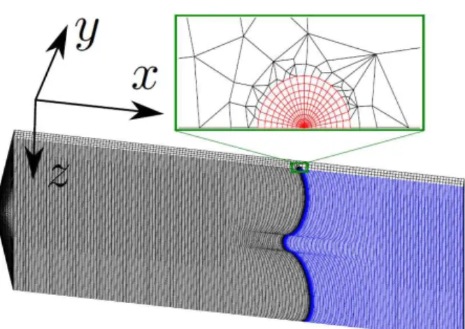
The simulations are performed with the FE code CAST3M developed by the French Commissariat `a l’ ´Energie Atomique (CEA). The values of Young’s modulus E = 71 GPa and Poisson’s ratio ν = 0.22 are those of glass for all the cleavage tests. The multilayer is neglected from a mechanical point of view due to its extremely low thickness compared to the glass plates. The results presented in this work correspond to meshes composed of 144,896 bilinear 8-node parallelepipedic elements and 180,471 nodes. The mesh of the glass plate is inhomogeneous. Its density increases as the displacement gradients, and thus especially in the vicinity of the crack tip. The mesh is refined until the displacement field converges at mechanical equilibrium. The mesh of the experimental crack front shape a(z) = a + δa(z) is obtained by deforming an invariant mesh in the z-direction of a straight crack front around its mean position a (Fig. 4). The mesh around the crack front is constructed to form a kind of regular cylinder around the front which is adapted to the “G-theta” method used to calculated the local ERR at each point of the front. This method developed by Destuynder and Djaoua (1981), allows us to calculate G accurately and quickly (Destuynder et al., 1983).
As output of the simulation, the 3D displacement fields obtained are used to obtain the local ERR G(z) along the front with the “G-theta” method. This method uses the displacement fields obtained by FE resolution of the elasticity problem. Due to the symmetry of the problem with respect to the x − z plane, i.e. the plane in which the crack propagates, only the upper glass plate located above the plane y = 0 is simulated. Symmetry boundary conditions are applied on this boundary. The boundary x = L is clamped. Stress free boundary conditions are applied on the rest of the boundary surfaces. Concerning the loading, a point displacement ∆ in the y-direction is applied on the triangular
Figure 4: Typical mesh of the cleavage test used in the finite element calculations. The unbroken interface is colored in blue. The highest mesh density corresponds to the crack front position. A zoom of the mesh in the vicinity of the crack tip is also reported in red.
tip as in the experiments. The value of ∆ is fixed so that the displacement at the corner δ of the sample shown in Fig. 2a converges toward the displacement measured experimentally. The final error between the experimental and numerical value of δ is less than 1%, i.e. less than the uncertainty of experimental measurement, for all crack configurations studied.
3.2. Evolution of the ERR during the propagation along the heterogeneous interface
The local ERRs are calculated along the crack fronts for all equilibrium positions of the crack obtained experi-mentally. In the following we illustrate our results in the case of the multilayer HC-b30 that exhibits the strongest adhesion contrast among the four types of interfaces presented in Sec. 2.
We plot the following results:
• The ERR landscape G(z) of a crack front trapped by the central defect strip (Fig. 5);
• The average ERR G0=< G(z) > as a function of the average position a of the crack front (Fig. 6a);
• The average fluctuations ∆G1and ∆G2of G(z) with respect to G0for interface areas situated outside and inside
the central defect strip respectively (Fig. 6b).
The evolution of the ERR landscape G(z) when the crack propagates is reported in Fig. 5a. The ERR contrast expected between the defect strip and its surrounding homogeneous medium is well reproduced by the ERR landscape. As reported in Fig. 3, three successive stages can be associated with this ERR landscape: homogeneous propagation (the front has a curved shape characteristic of finite width effect); interaction between the crack front and the central defect strip (the front is progressively deformed); stationary pinning (the deformation stays invariant in the direction of propagation).
A profile of the ERR G(z) obtained for a crack front trapped by the defect strip in the last stationary regime is shown in Fig. 5b. Despite the presence of some fluctuations, the presence of the central defect strip can be clearly identified and characterized by a significant variation of the ERR compared to average ERR G0. In the homogeneous and the
defect zones, the ERR is nearly constant longitudinally to the crack front in the direction z. It is therefore possible to attribute a characteristic ERR value for the two types of interfaces, homogeneous and defect strip, encountered by the crack. We note G1and G2 their respective average value from which we extract the corresponding mean variations
from ∆G1 = G1−G0and ∆G2 = G2−G0. The signs of ∆G1and ∆G2are by definition opposed. The notations G0,
G1, G2, ∆G1and ∆G2are reported on Fig. 5b.
Thanks to the FE calculations we compute the global ERR G0 by calculating the average ERR along the front
(a) -15 -10 -5 0 5 10 158 12 16 20 24 28 32 0 1 2 3 4 5 6 7 G(J/m2) I II III z(mm) x(mm) (b) -10 0 10 z (mm) 0 1 2 3 4 5 6 G (J/m 2 ) G0 G2 G1 ∆G 2 ∆G1
Figure 5: Local Energy Release Rate (ERR) computed by Finite Element (FE) for the cleavage test HC-b30. (a) Evolution of the ERR landscape. The three successive stages of propagation are distinguished as in Fig. 3. The ERR contrast expected between the defect strip and its surrounding homogeneous medium is well reproduced by the ERR landscape. (b) Local ERR along a crack front during regime III of Fig. 3. G0denotes the average along the front while
∆G1 and ∆G2denote the average variations of the energy release rate compared to G0outside and inside the defect
strip respectively. (a) 10 15 20 25 30 a (mm) 0.4 0.6 0.8 1 1.2 G0 (J/m 2 )
Regime I Regime II Regime III
(b) -5 0 5 10 a-a0 (mm) -0.5 0 1 2 3 4 ∆ G i (J/m 2 )
∆
G
2∆
G
1Figure 6: Energy Release Rate (ERR) calculated by finite element method (symbols) for the cleavage test HC-b30. In order to distinguish the three successive regimes of propagation the color code is same as in Fig. 3: black circles for the propagation along the homogeneous part of the interface, red squares for the transient regime and blue diamonds for the propagation in the patterned part of the interface. The error bars are deduced from statistical dispersions. (a) Mean ERR G0 evolution with the mean crack front position a. The continuous straight line corresponds to the
theoretical value deduced from the linear regression of Fig. 7 computed through Eq. 1. (b) ERR contrasts ∆Gi as a
function of the distance between the average crack front position and the beginning of the defect strip position a − a0.
The contrasts are calculated outside (∆G1) and inside (∆G2) the defect strip.
the average position of the crack in its direction of propagation a. These regimes correspond again to the morphology variations reported in Fig. 3. The average ERR G0is almost constant at the beginning and at the end of cleavage
test. Between these two ERR values a transient regime is observed. These three regimes correspond chronologically to the propagation of the crack front in a homogeneous medium, its interaction with the strip edges and finally to its stationary pinning by the defect strip. Changes in G0 reflect the change in the effective toughness of the interface
due to the presence of the defect strip during the crack propagation. The increase in G0 can be associated with a
The determination of local ERR values allows us to refine our understanding of the interaction between the crack front and the central defect strip. In Fig. 6b, we represent the variations ∆G1and ∆G2 as a function of the distance
between the average position of the crack a and the beginning of the masked zone a0in the crack propagation direction
x. The three regimes described above, from the change in G0, are considerably emphasized. We observe that the
variations ∆Gi are equal to zero for a − a0 < 0, i.e. before the interaction of the crack with the defect. During the
penetration of the strip by the crack front, in the vicinity of a − a0 = 0, ∆Givary dramatically. The ∆Gifinally reach
constant values for a − a0 >0 when the crack front is stationary trapped by the defect. Note that, in absolute value,
the variation ∆G1is about one order of magnitude lower than ∆G2. The width of the homogeneous zone is indeed an
order of magnitude greater than that the defect strip one. The signs of variations ∆Giare consistent with the observed
variations in G0. A defect strip whose adhesion is larger (smaller) than the homogeneous medium produces a variation
∆G2>0 (∆G2 <0) and ∆G1<0 (∆G1>0).
3.3. Simulation of the overall crack front curvature for an homogeneous interface
Even for a homogeneous pattern-free interface, for a sample of finite width b, the crack fronts are not exactly straight but adopt a curved shape (see wide dashed black lines in Fig. 3). This shape is due to the anticlastic defor-mation of the bent plates. To our knowledge, there is no simple analytical formula for modeling this contribution to the crack front shape. Therefore we have calculated the crack shape in an equivalent homogeneous medium cor-responding to the experimental geometry and loading. Using the FE method we have calculated crack shapes such that G(z) = G0along the front where G0is the average ERR computed previously by FE. The crack front shape is
determined from a mere steepest descent iterative algorithm. The equilibrium shape is reached when the difference between the local ERR G(z) and G0is less than 1% at any point of the front. These background curved shapes will
then be subtracted from the experimental fronts before analysis of the deformed crack fronts in the heterogeneous samples with the perturbation formulas (Sec. 5).
4. Analytical approaches
The idea here is to decompose the calculation of the local ERR along the deformed crack front as the sum of its global average value and its local increase along the perturbed configuration. Analytical methods allowing us to estimate the mean value (beam model) and the local relative values (perturbation methods) are presented in sections 4.1 and 4.2 respectively. Our goal is here to be able to determine the ERR landscape analytically in order to compare theoretical predictions with previous FE numerical calculations in sections 5 and 6.
4.1. Determination of the average ERR
The first step of our theoretical study is to determine the global ERR, i.e. the mean ERR G0. A standard data
analysis is to calculate G0by a simple beam bending model at fixed displacement (Fig. 2b). According to Kanninen
(1973), the ERR in a state of plane stress reads:
G0=
3Eh3δ2
16(a + 0.64h)4. (1)
Note that the geometry of the problem meets the assumptions leading to Eq. 1, i.e. a ≫ h and L − a > 2h, for all the cleavage tests studied in this work. We need to adapt the beam model to pass from a three-dimensional elastic problem to a beam model in one dimension. Kanninen’s model is therefore employed using the average crack front position a calculated along the width of the plate in the z direction. This average position is obtained directly from experimental crack front positions a(z).
In practice, we plot the evolution of δ2 as a function of (a + 0.64h)4. In Fig. 7, the case of sample HC-b30 is reported as an example. In this kind of graph, G0 is simply proportional to the slope of the curve. We can clearly
identified the three different regimes described in Sec. 3.2.
We extract the nearly constant value of G0 in regime III, i.e. where the the pinning is stationary, by a linear
regression procedure. In the case of sample HC-b30, we obtain G0 = 0.95 ± 0.14 J/m2 as reported in Fig. 7. This
quantity will be used to determine adhesion properties in Sec. 6. The comparison with FE numerical calculations in Fig. 6a shows a good agreement.
0 4 8 12 16(a+0.64h)4 (mm4) 0 4 8 12 3Eh 3 δ 2 (N.mm 3 )
Regime I Regime II Regime III
x106
x10
6
G0= 0.95 J/m2
Figure 7: Typical data plot according to Kanninen’s model for the cleavage test HC-b30. The slope corresponds to the mean Energy Release Rate (ERR) G0. The three successive regimes of propagation are distinguished as in Fig. 3.
I: stationary propagation along the silver homogeneous interface (black circles); II: transient deformation of the front when entering the defect strip (red squares); III: stationary propagation of the deformed front in the defect strip (blue diamonds). The straight line is a linear regression of the data in the regime III.
For all the experiments, the variations of G0 due to the interaction between the crack and the defect are well
reproduced by Eq. 1 as a function of the average position of the crack front. G0is only slightly underestimated with
respect to FE calculations. The maximum relative error between the beam model predictions and the FE numerical calculations remains below 10% for all samples. This result validates the use of Kanninen’s model to evaluate G0in
our system.
4.2. Perturbation method
We now present the perturbation approaches to model the cleavage test. Our goal is to evaluate the local ERRs from the knowledge of the crack front morphology a(z), this time using a lightweight analytical method. We first discuss the formulas giving the first order variation of the local ERR due to a perturbation of the crack front position. We then customize them to our experiments: we assume that the ERR landscape is stepwise to reduce the determination of the local ERR to a single parameter, namely the ERR contrast. The usefulness of those formulas appears when applied to the experiments, since they allow to reduce the errors linked to the local noise of measures in the crack front position a(z).
4.2.1. Variation of the local ERR due to small crack front perturbations
Two different cases are considered: 1) when the wavelength λ of the crack front perturbation is small compared to the plate thickness, that is when the medium can be supposed to be infinite and 2) when λ is large, that is when a thin plate model can be used.
• Rice (1985)’s formula for a half-plane crack in an infinite medium: In his pioneer work Rice (1985) has
calculated the theoretical expression of the ERR first-order variation δG(z) along a planar crack front due to a small perturbation of the front position δa(z). This expression is valid in principle for a semi-infinite crack in an infinite body. From the perspective of a DCB geometry (see Fig. 2a), such a geometric mapping is acceptable if the characteristic perturbation length λ of the crack front meets the conditions: λ ≪ h and λ ≪ a. The first condition implies that the plate must be very thick with respect to the perturbation wavelength. Provided that these assumptions are met and that the load is invariant along the crack front in the z direction, cδG(k) is given in Fourier space by:
c δG(k) G0 = F∞(k, a) bδa(k) with F∞(k, a) = (−|k| + 1 G0 dG da), (2)
where λ = 2π/|k| is the wavelength of the front perturbation and G0 the ERR of the straight crack front of average
position a. Note that to first order G0 corresponds to the average ERR as introduced in the previous sections. The
derivative dG/da is calculated in our work from the simple Euler-Bernoulli beam model (Tada et al., 1985) consistent with the plate model presented subsequently. In this case, the variation 1/G0.(dG/da) with the crack length a is merely
given by −4/a.
•Legrand et al. (2011)’s formula for a half-plane crack in a thin plate
Rice’s method has been extended by Legrand et al. (2011) adapting it to the case of a semi-infinite planar crack located in the mid-plane of a thin plate. This system satisfies the conditions: λ ≫ h and h ≪ a. Under these assumptions, the perturbation of the crack can be treated with the Love-Kirchhoff theory for thin plates, which greatly reduces the complexity of the problem. Note that in this case, the first condition implies that the plate must be very thin with respect to the perturbation wavelength. The first order variation of the ERR in Fourier space writes as follows:
c δG(k)
G0
= FPlate(ka) bδa(k) with Fplate(ka) =
2 a
2ka cosh(2ka) − sinh(2ka) 2ka − sinh(2ka)
!
. (3)
4.2.2. Application to a stepwise ERR landscape
The cleavage experiments can be modeled by assigning characteristic ERRs to the homogeneous area (G1) and
defect strip (G2). This assumption seems very reasonable from FE numerical results of Sec. 3.2. In the presence of a
defect of known width d, the ERR landscape is modeled by:
G(z) = G0+ Π1(z)∆G1+ Π2(z)∆G2 with
(
Π1= 0, Π2= 1 if |z| < d/2
Π1= 1, Π2= 0 if |z| > d/2
, (4)
where Πiare rectangular functions. The variation of the normalized ERR is:
δG(z) G0 =∆G1 G0 Π1(z) + ∆G2 G0 Π2(z). (5)
The average G0 provides a relation linking the ERR of the defect strip and the surrounding homogeneous medium.
Denoting G1the ERR in the homogeneous zone and G2the ERR in the defect strip, we assume that G0is an average
along the front line, which we simply write as:
G0=
G1(b − d) + G2d
b . (6)
We can write Eq. 5 in Fourier space to deduce the front shape δa(z) from Eqs. 2 or 3. Using Eq. 6 to express ∆G2
as a function of ∆G1, we obtain: b δa(k) = 1 F(k, a) ∆G2 G0 h −d/(b − d)cΠ1(k) + cΠ2(k) i , (7)
where F(k, a) is one of the elastic kernels from Eqs. 2 or 3. Eq. 7 establishes a relationship which relates the shape of the crack front with the ERR contrasts between the defect strip and the homogeneous medium in the present geometry.
5. Determination of ERR contrasts
In the previous sections, we have presented experimental front morphologies in homogeneous and patterned inter-faces, along with thorough FE modeling to access both global ERR and ERR distribution over the sample. We now analyze the same data with the analytical formulas derived from the perturbation method.
5.1. Corrections of experimental crack front positions
In order to apply the perturbation approaches to calculate the local ERR, it is first necessary to correct the experi-mental front shapes a(z)Exp = a + δa(z)Expfrom extrinsic effects that were not taken into account in the perturbation
method. This task is equivalent to determining the unperturbed crack front geometry and its variation with crack length δa(z) in the absence of defect strip. Indeed, the perturbation approaches described in Sec. 4.2 apply only to a solid which is infinite in the lateral (z) direction, i.e. an infinite straight crack front. In the experiments, the finite width of the sample induces a curvature of the front due to the anticlastic effect as presented in Sec. 3.3. In order to take into account this additional finite size effect, we take as unperturbed reference crack front, for a given global G0
level, the curved front a(z)Anti= a + δa(z)Anticalculated by the FE simulations method presented in Sec. 3.3.
-15 -10 -5 0 5 10 15 z (mm) -2 -1.5 -1 -0.5 0 0.5 δ aAnti (mm) a=12.48 mm a=18.44 mm a=28.72 mm
Figure 8: Variation of the crack front position calculated by the finite element method for an equivalent homogeneous medium whose curvature comes from anticlastic coupling. The obtained shapes are exemplified for the HC-b30 cleavage test for different mean crack front positions. Note that the scale of the axes are different. The front is almost straight.
Examples of curved fronts obtained by this method for the HC-b30 cleavage test are shown in Fig. 8. These shapes are characteristic of curved crack fronts in homogeneous specimens of finite width (Jumel and Shanahan, 2008). Note that, due to the changes of the ratio a/b, and thus the stress state with the advance of the crack, the curvature of the crack depends on the average crack length as expected. The loading on the triangular tip of the plates also reinforces the crack front curvature variation. This curvature variation shown in Fig. 8 emphasizes that the influence of the width of samples is not constant as assumed in Dalmas et al. (2009). It clearly depends on the the mean crack length a. The solutions obtained will serve us as the reference unperturbed solutions in the perturbation approaches presented below.
A second correction comes from a slight rotation around the x-axis of the wedge between the plates during loading which induces an imperfect symmetry with respect to the plane z = 0 at the center of the sample. This lack of symmetry is reflected by a slight linear bias in z of the crack position. For instance, the crack front shape, corrected from the anticlastic effect, in a homogeneous medium is a linear function of z instead of being completely flat with
δa(z) = 0 for all points along the front. We choose to correct this load-related effect by subtracting a linear fit δa(z)Lin
to the experimental position. This procedure partially restores the symmetry of the problem with respect to the plane z=0 at the center of the specimen as assumed in the model described in the previous theoretical section. Note that it does not affect the ERR contrast calculation, but merely allows a better fit of the elastic line model on experimental data.
The variation of the position of the crack front around its average position a corrected from both anticlastic and rotation effects writes:
δa(z) = δa(z)Exp−δa(z)Anti−δa(z)Lin. (8)
An example of a corrected crack front morphology in regime III for the HC-b30 sample is shown in Fig. 9. The impact of the defect strip on the front morphology is clearly visible. Consistent with the FE analysis of Fig. 5 and 6,
-15 -10 -5 0 5 10 15 z (mm) -2 -1.5 -1 -0.5 0 0.5 1 δ a (mm)
Thin plate model Semi-infinite model
Figure 9: Variation of the experimental crack front positions (symbols) corrected through Eq. 8 for the cleavage test HC-b30. The dashed and solid curves correspond to the fitted semi-infinite (Eq. 2) and thin plate (Eq. 3) models, respectively. Note that the vertical axis is expanded approximatively ten times compared to the horizontal axis.
an increase in ERR corresponds to the anchoring of the crack. Note that the ordinate axis of Fig. 9 is approximatively expanded ten times in comparison with the axis of abscissa. This observation reflects the fact that the perturbations of the crack front position are small compared to the width of the specimen. The morphologies of experimental crack fronts therefore justify a priori a theoretical treatment based on a first-order perturbative approach presented in Sec. 4.2.
5.2. Quantitative analysis of crack front deformations with perturbation methods
In order to reproduce the shape of the experimental crack front with Eq. 7, we have chosen to work in the direct space by adjusting the single free parameter ∆G2/G0. Indeed, the presence of experimental noise on the crack front
position makes the determination of the ERR contrast difficult from a direct use of Eq. 7 in Fourier space. The normalized ERR contrast is determined by minimizing the mean square error between the experimental front shape and the front morphology predicted after a numerical transformation into real space of Eq. 7. This adjustment procedure has fewer degrees of freedom than in the work of Dalmas et al. (2009) where the width of the defect strip was taken as a free parameter.
The morphologies of the fronts obtained from the best fit of the different elastic kernels are plotted in Fig. 9. Both perturbative approaches satisfactorily reproduce the crack front shapes except near the edges of the specimen due to free surface effects. Fig. 9 shows only a slight better agreement with the experimental results for the thin plate model. In order to get quantitative interpretation, the average mean square error over all the crack configurations for the four samples has been computed for both models. We found that the error on the experimental crack front positions is lower in average for the thin plate model than for the semi-infinite model. It seems difficult however to find a significant difference between the semi-infinite and thin plate formulas on the basis of the front morphology. In the next section we will see that quasi-equivalent front shapes in fact involve very different ERR contrasts allowing us to judge of the applicability of the models.
5.3. Comparison between perturbation methods and FE results
The fitting procedure presented above gives us the opportunity to access local ERR contrasts, i.e. to the difference of ERR between the defect strip and its homogeneous environment. From this adjustment we can calculate the normalized contrasts ∆G2/G0 directly through Eq. 7. ∆G1/G0 is then deduced from ∆G2/G0 through Eq. 6. This
last step completes the determination of the ERR landscape by the perturbation method, knowing the geometry of the system, especially the crack front morphology and the defect strip width.
As expected from the theoretical work of Legrand et al. (2011), the absolute values of ERR contrasts predicted by the semi-infinite model are found to be lower than those predicted by the thin plate model. The ratio between the
latter and the former is about 2.5. To discriminate between the two elastic line models, we compare their respective predictions with the numerical FE calculations.
-0.5 0 1 2 3 4
∆Gi/G0 from finite element calculations
-0.5 0 1 2 3 4 ∆ G i /G 0
from perturbation approaches
LC-b40 MC-b50 MC-b40 HC-b30
Figure 10: Comparison of normalized Energy Release Rate (ERR) contrasts ∆Gi/G0calculated by the finite element
method with those obtained from the semi-infinite (red open symbols) and the thin plate (black solid symbols) the-oretical approaches. The blue dotted lines correspond to the perfect equivalence between these two quantities. The error bars are deduced from statistical dispersions.
Comparisons between the ERR contrasts deduced from theoretical approaches with the FE results are shown in Fig. 10 where the results obtained for all crack fronts of the four samples LC-b40, MC-b40, MC-b50, and HC-b30. Despite some discrepancies, Fig. 10 shows a much better description of the ERR contrasts when the plate model is used. The average relative error on ∆Gi/G0for all the data of Fig. 10 in comparison with the FE results decreases
from 61% when Rice’s model is applied directly as for a semi-infinite medium to 16% when the finite thickness of the plate is taken into account.
Despite a correct description of the front shapes of the pinned cracks, Rice’s model as applied directly to the present DCB tests systematically underestimates the ERR normalized contrasts. This result comes from the fact that the perturbation wavelengths of the crack front are much larger than the specimen thicknesses. This is often encountered in the literature when thin plate geometries is used to study interfacial crack propagation. Therefore, in such geometries, it is necessary to model the cracks by taking into account the finite thickness of the plate, as shown by Legrand et al. (2011). Using this model, we find quantitative agreement, i.e. within the error bars, with the three dimensional FE calculations.
In the more general case, Legrand et al. (2011) have also developed a model that connects both regimes (semi-infinite and thin plate) as a function of the wavelength of the perturbations relative to the thickness of the specimen. This more general kernel is not relevant here since the width of the defect is much larger than the plate thickness h, so that we always stand in the vicinity of the thin plate limit.
6. Crack front propagation and material properties
6.1. Propagation criterion
Thanks to our experimental procedure, the interpretation of the previous results in terms of material properties, i.e. adhesion, is fairly straightforward. Indeed, due to the quasi-static propagation of the crack, a propagation criterion has to be fulfilled at any point of the observed front. For a given load, the crack front stops at locations where the propagation driving force is no longer sufficient. It is common for brittle fracture to assume that the crack front advance is ruled by the Griffith criterion. In this framework, the equilibrium morphology of the crack front a(z) = a + δa(z) for a given opening δ obeys:
Sample Stack Finite element (J.m−2) Rice model (J.m−2) Plate model (J.m−2) LC-b40 Gl./Org/Ag/Si3N4 0.35 ± 0.04 0.46 ± 0.19 0.32 ± 0.13
MC-b40 Gl./Si3N4/Ag/Si3N4 1.57 ± 0.11 1.13 ± 0.09 1.52 ± 0.14
MC-b50 Gl./Si3N4/Ag/Si3N4 1.86 ± 0.12 1.16 ± 0.12 1.75 ± 0.18
HC-b30 Gl./Ag/Si3N4 4.63 ± 0.31 2.23 ± 0.36 4.09 ± 0.64
Table 2: Average adhesion energy of the different defect strip interfaces G2c = G0+ ∆G2computed by FE analysis,
perturbation theory using Rice (semi-infinite geometry) and Legrand (plate geometry) formulas respectively.
where Gc(z) is the local adhesion energy. Therefore, we can deduce the fracture energies of both the surrounding
homogeneous medium and the defect strip interfaces denoted G1c and G2c respectively. In a very similar way, the
adhesion energy has been measured for homogeneous interfaces by Barthel et al. (2005).
While the data of the crack front geometry and the loading geometry can give a direct access to the ERR G(z), the same is not systematically true for the adhesion energy Gc(z). It would be the case if the arrest condition for a
crack front Eq. 9 was an equality and not only a simple inequality. Thus, the fracture energy can only be deduced from the ERR for stationary crack propagation regimes, i.e. where the materials properties are invariant in the crack propagation direction (Roux et al., 2003). In our system, it is the case for the regimes I and III described previously. Between these two stationary regimes a transient regime (II) is observed where the inequality of Eq. 9 remains and the determination of Gc(z) is not possible.
In the first regime (stage I of Fig. 3), the crack propagates in a completely homogeneous zone and G1 = G1c
along the front. When the crack begins to interact with the obstacle (stage II of Fig. 3), G2 ≤G2cin the defect strip
and G2 increases with the applied load involving a significant change in ∆Gi. Once the defect is penetrated by the
crack G2 = G2cin strip and, for each increment of the opening, the crack advances with ∆Ginearly constant. In this
last stationary regime of crack propagation (stage III in Fig. 3) the toughness contrast is invariant in the direction of propagation, and we have equality between the local values of adhesion energy and ERR all along the front. The present methods can then be used to measure interfacial toughness in the defect strip.
Note that it is also possible to simulate the quasi-static propagation of a crack for a given toughness landscape. The adhesion energy of the defect strip and its surrounding homogeneous medium could be obtained by adjusting their values in order to reproduce the shape of the crack front observed experimentally. This procedure is however computationally demanding as it implies to describe the propagation of the crack which involves the calculation of a large number of configurations. In this study, the aim was not to perform propagation simulations of the crack, but to validate the analytical perturbation approach, hence it was enough to take advantage of our experimental setup which offers a direct observation of the crack front equilibrium shape and to perform direct simulations of the elastic problem for each equilibrium configuration.
6.2. Determination of the defect strip adhesion
In this last section we leverage the originality of this work by focusing on the determination of the defect strip adhesion G2cin the framework of crack pinning in heterogeneous interfaces. The measurement of G2cis carried out
in the regime III where the crack front pinning is invariant in the direction of propagation.
In this regime, we compute the fracture energy G2cas the sum of global ERR plus the average ERR fluctuation in
the defect strip G0+ ∆G2. Since G2cfluctuates due to experimental noise we choose to compute its average G2cover
all the crack front configurations belonging to the last stationary pinning regime (blue diamond symbols in Fig. 6). In the case of FE numerical calculations, G2cis simply computed from the mean local ERRs G(z) in the defect strip
as presented in Sec. 3.2. In the case of analytical approaches, G0 is computed with Eq. 1 (Sec. 4.1) while ∆G2 are
determined through the fit of the experimental crack front positions by the two perturbation approaches (Sec. 5.2). We finally computed G2cby averaging G0+ ∆G2.
The results are summarized in Tab. 2. As expected following the conclusions about ERR contrasts of the previous section, the semi-infinite model predictions deviate significantly from the FE results summarized in Tab. 2. In turn, we observe a very satisfactory agreement between the values obtained from perturbative approaches using the plate model and the values calculated by FE. The agreement is even quantitative, i.e. inside the error bars, for the samples LC-b40, MC-b40 and MC-b50. Moreover, nearly identical adhesion energies are found for the MC-b40 and MC-b50
samples due to the identical nature of their cracked interfaces as reported in Tab. 1. The adhesion energy for the defect strip of sample HC-b30 is slightly out of the margins of error calculated. This interface presents however the largest adhesion contrast of the four samples studied. One interpretation could therefore reside in the fact that in the latter case we touched the limits of first-order perturbative approaches.
As a result, our approaches based on the patterning of a weak interface can be considered as a new method to determine the adhesion energy of heterogeneous interfaces for transparent materials by measuring the crack front deformation that it induces.
7. Summary and perspectives
We have shown how the results of cleavage test experiments can be thoroughly analyzed by FEM. The ERR has been computed for all the measured crack front and a consistent picture of the crack propagation in the heterogeneous interface has been reconstructed. This analysis of the data is particularly illuminating when considering the increasing deformation of the crack front as it hits the edge of the high toughness area as it progresses forward. Due to the increasing curvature of the crack front, the local energy release rate rises until it reaches the toughness of the pinning area which then starts to rupture.
This relation between front curvature and local energy release rate is at the core of the perturbation method pro-posed by Rice. Fitting the front with a perturbation kernel is a much lighter way of analyzing the data. Here we have demonstrated that plate thickness is a first order parameter in modelling crack front morphology by perturbation methods when the wavelengths of the perturbation are comparable to the plate thickness. In our experimental configu-ration, the semi-infinite kernel (Rice) gives results which are only qualitatively correct, while the agreement is clearly improved when the finite plate thickness kernel is used.
Our study, combining experiments, numerical simulations and theoretical analysis shows that it is possible to describe quantitatively the local adhesion contrasts only from the observed crack front morphologies taking into account the whole problem geometry. As a result, it can serve as a method to characterize the local toughness of transparent materials.
To improve the description of the depinning threshold for crack propagation in heterogeneous brittle materials two directions of investigation can be naturally considered from this work. The first one is to develop an approach capable of handling the anticlastic effect analytically (Jumel and Shanahan, 2008). Under this condition, our approach could be more effective and avoid any numerical simulations. A second perspective is related to the size of the perturbation induced by the heterogeneity of the material. Elastic line models presented in this paper are indeed limited by a first order perturbative approach. If it seems that it can account for adhesion contrasts up to 4 J/m2, we expect a loss of
validity as the toughness contrast increases. Approaches including higher orders in perturbation (Rice, 1989; Bower and Ortiz, 1991; Lazarus, 2003; Favier et al., 2006; Leblond et al., 2012) could be a solution and should allow to treat much higher adhesion contrasts.
Acknowledgements
The support of the ANR Programme SYSCOMM (ANR-09-SYSC-006) is gratefully acknowledged.
References
Barthel, E., Kerjan, O., Nael, P., Nadaud, N., 2005. Asymmetric silver to oxide adhesion in multilayers deposited on glass by sputtering. Thin Solid Films 473, 272–277.
Bonamy, D., 2009. Intermittency and roughening in the failure of brittle heterogeneous materials. Journal of Physics D: Applied Physics 42, 214014.
Bouchaud, E., 1997. Scaling properties of cracks. Journal of Physics: Condensed Matter 9, 4319–4344.
Bower, A.F., Ortiz, M., 1991. A three-dimensional analysis of crack trapping and bridging by tough particles. Journal of the Mechanics and Physics of Solids 39, 815–858.
Bueckner, H.F., 1987. Weight functions and fundamental fields for the penny-shaped and the half-plane crack in three-space. International Journal of Solids and Structures 23, 57–93.
Chopin, J., Prevost, A., Boudaoud, A., Adda-Bedia, M., 2011. Crack front dynamics across a single heterogeneity. Preprint .
Dalmas, D., Barthel, E., Vandembroucq, D., 2009. Crack front pinning by design in planar heterogeneous interfaces. Journal of the Mechanics and Physics of Solids 57.
Dalmas, D., Lelarge, A., Vandembroucq, D., 2008. Crack propagation through phase-separated glasses: Effect of the characteristic size of disorder. Phys. Rev. Lett. 101, 255501.
Delaplace, A., Schmittbuhl, J., Måløy, K.J., 1999. High resolution description of a crack front in a heterogeneous plexiglas block. Physical Review E 60, 1337.
Destuynder, P., Djaoua, M., 1981. Sur une interpr´etation math´ematique de l’int´egrale de rice en th´eorie de la rupture fragile. Mathematical Methods in the Applied Sciences 3, 7087.
Destuynder, P., Djaoua, M., Lescure, S., 1983. Quelques remarques sur la m´ecanique de la rupture ´elastique. Journal de M´ecanique Th´eorique et Appliqu´ee 2.
Favier, E., Lazarus, V., Leblond, J.B., 2006. Coplanar propagation paths of 3D cracks in infinite bodies loaded in shear. International Journal of Solids and Structures 43, 2091–2109.
Gao, H.J., 1988. Nearly circular shear mode cracks. International Journal of Solids and Structures 24, 177–193. Gao, H.J., Rice, J.R., 1987. Nearly circular connections of elastic half spaces. Journal of Applied Mechanics 54, 627.
Gao, H.J., Rice, J.R., 1989. A First-Order perturbation analysis of crack trapping by arrays of obstacles. Journal of Applied Mechanics 56, 828–836.
Griffith, A.A., 1921. The phenomena of rupture and flow in solids. Philosophical Transactions of the Royal Society of London A 221, 163198. Irwin, G., 1957. Analysis of stresses and strains near the end of a crack traversing a plate. Journal of Applied Mechanics 24, 361364. Jumel, J., Shanahan, M.E.R., 2008. Crack front curvature in the wedge test. The Journal of Adhesion 84, 788–804.
Kanninen, M.F., 1973. An augmented double cantilever beam model for studying crack propagation and arrest. International Journal of Fracture 9, 83–92.
Lazarus, V., 2003. Brittle fracture and fatigue propagation paths of 3d plane cracks under uniform remote tensile loading. International Journal of Fracture 122, 23–46. 10.1023/B:FRAC.0000005373.73286.5d.
Lazarus, V., 2011. Perturbation approaches of a planar crack in linear elastic fracture mechanics: A review. Journal of the Mechanics and Physics of Solids 59, 121–144.
Lazarus, V., Leblond, J., 2002. In-plane perturbation of the tunnel-crack under shear loading I: bifurcation and stability of the straight configuration of the front. International Journal of Solids and Structures 39, 4421–4436.
Leblond, J.B., Mouchrif, S.E., Perrin, G., 1996. The tensile tunnel-crack with a slightly wavy front. International journal of solids and structures 33.
Leblond, J.B., Patinet, S., Frelat, J., Lazarus, V., 2012. Second-order coplanar perturbation of a semi-infinite crack in an infinite body. Engineering Fracture Mechanics 90, 129 – 142.
Legrand, L., Patinet, S., Leblond, J., Frelat, J., Lazarus, V., Vandembroucq, D., 2011. Coplanar perturbation of a crack lying on the mid-plane of a plate. International Journal of Fracture 170, 67–82.
Måløy, K.J., Schmittbuhl, J., 2001. Dynamical event during slow crack propagation. Physical Review Letters 87.
Mower, T.M., Argon, A.S., 1995. Experimental investigations of crack trapping in brittle heterogeneous solids. Mechanics of Materials 19, 343–364.
Pindra, N., Lazarus, V., Leblond, J.B., 2010. In-plane perturbation of a system of two coplanar slit-cracks-I: case of arbitrarily spaced crack fronts. International Journal of Solids and Structures .
Ponson, L., Auradou, H., Pessel, M., Lazarus, V., Hulin, J.P., 2007. Failure mechanisms and surface roughness statistics of fractured fontainebleau sandstone. Physical Review E 76.
Rice, J.R., 1985. First-Order variation in elastic fields due to variation in location of a planar crack front. Journal of Applied Mechanics 52, 571–579.
Rice, J.R., 1989. Weight function theory for three-dimensional elastic crack analysis. In: Wei,R.P., Gangloff, R.P.(Eds.), Fracture Mechan-ics:Perspectives and Directions (Twentieth Symposium). American Society for Testing and Materials STP1020, Philadelphia, USA , 29. Roux, S., Vandembroucq, D., Hild, F., 2003. Effective toughness of heterogeneous brittle materials. European Journal of Mechanics - A/Solids 22,
743–749.
Santucci, S., Grob, M., Toussaint, R., Schmittbuhl, J., Hansen, A., Måløy, K.J., 2010. Fracture roughness scaling: A case study on planar cracks. EPL (Europhysics Letters) 92, 44001.
Santucci, S., Måløy, K.J., Delaplace, A., Mathiesen, J., Hansen, A., Haavig Bakke, J.O., Schmittbuhl, J., Vanel, L., Ray, P., 2007. Statistics of fracture surfaces. Phys. Rev. E 75, 016104.
Schmittbuhl, J., Måløy, K.J., 1997. Direct observation of a self-affine crack propagation. Physical review letters 78.
Tada, H., Paris, P.C., Irwin, G.R., 1985. The stress analysis of cracks handbook. The American Society of Mechanical Engineers, New York. 3 edition.
Tallakstad, K.T., Toussaint, R., Santucci, S., Schmittbuhl, J., Måløy, K.J., 2011. Local dynamics of a randomly pinned crack front during creep and forced propagation: An experimental study. Physical Review E 83, 046108.