HAL Id: hal-00296480
https://hal.archives-ouvertes.fr/hal-00296480
Submitted on 7 Mar 2008
HAL is a multi-disciplinary open access
archive for the deposit and dissemination of
sci-entific research documents, whether they are
pub-lished or not. The documents may come from
teaching and research institutions in France or
abroad, or from public or private research centers.
L’archive ouverte pluridisciplinaire HAL, est
destinée au dépôt et à la diffusion de documents
scientifiques de niveau recherche, publiés ou non,
émanant des établissements d’enseignement et de
recherche français ou étrangers, des laboratoires
publics ou privés.
analysis of changes in the specific absorption of
elemental carbon
J. C. Doran, J. D. Fast, J. C. Barnard, A. Laskin, Y. Desyaterik, M. K. Gilles
To cite this version:
J. C. Doran, J. D. Fast, J. C. Barnard, A. Laskin, Y. Desyaterik, et al.. Applications of lagrangian
dis-persion modeling to the analysis of changes in the specific absorption of elemental carbon. Atmospheric
Chemistry and Physics, European Geosciences Union, 2008, 8 (5), pp.1377-1389. �hal-00296480�
www.atmos-chem-phys.net/8/1377/2008/ © Author(s) 2008. This work is distributed under the Creative Commons Attribution 3.0 License.
Chemistry
and Physics
Applications of lagrangian dispersion modeling to the analysis of
changes in the specific absorption of elemental carbon
J. C. Doran1, J. D. Fast1, J. C. Barnard1, A. Laskin1, Y. Desyaterik1, and M. K. Gilles2
1Pacific Northwest National Laboratory, P.O. Box 999, Richland, Washington, 99354, USA 2Lawrence Berkeley National Laboratory, Berkeley, CA, USA
Received: 25 September 2007 – Published in Atmos. Chem. Phys. Discuss.: 19 October 2007 Revised: 17 January 2008 – Accepted: 12 February 2008 – Published: 7 March 2008
Abstract. We use a Lagrangian dispersion model driven by
a mesoscale model with four-dimensional data assimilation to simulate the dispersion of elemental carbon (EC) over a region encompassing Mexico City and its surroundings. The region was the study domain for the 2006 MAX-MEX ex-periment, which was a component of the MILAGRO cam-paign. The results are used to identify periods when biomass burning was likely to have had a significant impact on the concentrations of elemental carbon at two sites, T1 and T2, downwind of the city, and when emissions from the Mexico City Metropolitan Area (MCMA) were likely to have been more important. They are also used to estimate the median ages of EC affecting the specific absorption of light, αABS, at
870 nm as well as to identify periods when the urban plume from the MCMA was likely to have been advected over T1 and T2. Median EC ages at T1 and T2 are substantially larger during the day than at night. Values of αABS at T1,
the nearer of the two sites to Mexico City, were smaller at night and increased rapidly after mid-morning, peaking in the mid-afternoon. The behavior is attributed to the coating of aerosols with substances such as sulfate or organic carbon during daylight hours, but such coating appears to be limited or absent at night. Evidence for this is provided by scan-ning electron microscopy images of aerosols collected at the sampling sites. During daylight hours the values of αABSdid
not increase with aerosol age for median ages in the range of 1–4 h. There is some evidence for absorption increasing as aerosols were advected from T1 to T2 but the statistical significance of that result is not strong.
Correspondence to: J. D. Fast (jerome.fast@pnl.gov)
1 Introduction
It is generally acknowledged that as soot particles age, their mixing state evolves from an external to an internal one through processes such as heterocoagulation or condensation (e.g., Jacobson and Seinfeld, 2004), and the specific absorp-tion αABS (absorption per unit mass) will increase (Fuller
et al., 1999; Bond et al., 2006.) It is important to specify appropriate values of αABS for use in global climate
mod-els, but there is still considerable variation in the values that have been proposed. Bond and Bergstom (2006) concluded that αABS for freshly emitted soot particles has a value of
7.5±1.2 m2g−1 at 550 nm, but direct measurements in the field of the rates and effects of aging and coating have been difficult to achieve.
One approach has been to make comparisons of optical properties of soot at a single site at two different times of day, e.g., in the early morning when fresh emissions from traffic are likely to dominate the aerosol mix, and later in the afternoon when a mixture of fresh and more aged particles is likely to be present. The sources and ages of the various components of the mixture may vary widely, however, and efforts to explicitly characterize the ages of the mixture are not usually made. Several investigations of this type have been done in the Mexico City region, which is the location of interest for this study. Johnson et al. (2005) showed that soot can undergo significant coating and evolve into an inter-nally mixed state in only a few hours. In contrast, Mallet et al. (2004) concluded that single scattering albedo measure-ments in an industrial region of France were more consistent with externally mixed aerosols rather than internally mixed ones. Baumgardner et al. (2000) measured time series of size distribution, scattering and absorption coefficients, and bulk chemical composition of aerosols at a mountain location near Mexico City and related the variations to the meteorological conditions. Baumgardner et al. (2007) measured variations in αABS and in the coating of light absorbing carbon (LAC)
32
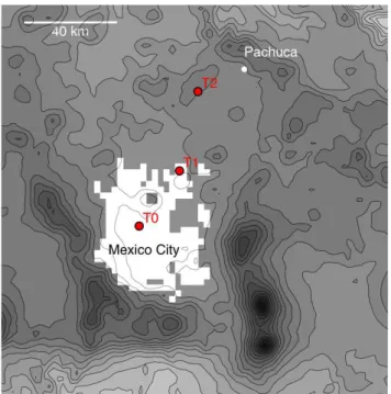
Fig. 1. Map of the study area, including the locations of the
sam-pling sites T0, T1, and T2 and the extent of the Mexico City Metropolitan Area (MCMA). Topography contour intervals are 200 m.
at an urban location in Mexico City. They found that αABS
changed relatively little during the day, reaching its mini-mum values when the LAC mass reached its peak around 08:00 LST.
Another approach to the study of aging effects on αABS
has been to measure soot properties at several sites that are likely to be characterized by particles with different ages, but actual ages are not normally estimated (e.g., Burtscher et al., 1993). Still another approach involves Lagrangian sampling in which an air parcel containing soot is followed from its source to some downwind location, monitoring the mixing state and optical properties of the soot en route. This may be straightforward for point sources (e.g., biomass burning) but can be problematic for more dispersed sources such as a large urban area or when additional sources contribute to the contents of the air parcel en route. Moteki et al. (2007) found that black carbon became internally coated on a time scale of 12 h in an urban plume downwind of Nagoya, Japan.
Riemer et al. (2004) used meteorological, chemical, and aerosol modeling to simulate the aging of diesel soot and study its evolution from an external to an internal mixture for summer conditions in southwestern Germany. They found that the time scale for the aging process was as short as a few hours during the day and was considerably longer at night, but no estimates of the effect on αABSwere discussed.
Com-parisons of aerosol residence times in the atmosphere using this scheme with times from other aging schemes in an at-mospheric general circulation model are described by Croft et al. (2005).
A complementary approach to these methods, which we describe in this paper, is to make use of a mesoscale model incorporating four-dimensional data assimilation to help in-terpret results from field measurements of αABS. In March of
2006 we made measurements of αABS at two sites, labeled
T1 and T2 and separated by approximately 35 km, down-wind of Mexico City. If the time scale for the coating of soot is only a few hours, we would expect that this sepa-ration would be sufficient to result in a significant change in αABS between T1 and T2; if the time scale is on the
or-der of 12 h or more, the changes would be negligible. The T1-T2 measurements were part of the MAX-Mex (Megac-ity Aerosol Experiment in Mexico C(Megac-ity; http://www.asp.bnl. gov/MAX-Mex.html) component of the MILAGRO (Megac-ity Initiative: Local and Global Research Observations; http: //www.eol.ucar.edu/projects/milagro/) field campaign. MI-LAGRO was designed to follow the downwind transport of the urban plume emanating from Mexico City and its surroundings and to study the transformation of gases and aerosols over scales ranging from 10 s of km to 1000 km and more. The MAX-Mex campaign focused on aerosols on lo-cal to regional slo-cales. A description of the T1-T2 campaign and some preliminary results have been given in Doran et al. (2007) and Doran (2007), so only a brief summary of it is provided below.
Figure 1 shows a map of the study area, including the loca-tions of the T1 and T2 sampling sites, the location of a third sampling site in an industrial area with heavily trafficked roads closer to the city center, T0, and the extent of the Mex-ico City Metropolitan Area (MCMA). Sunset Laboratory Or-ganic and Elemental Carbon (OCEC) analyzers (Birch and Cary, 1996) were deployed at T1 and T2, as were photoa-coustic absorption spectrometers (PASs) operating at a wave-length of 870 nm (Arnott et al., 1999, 2003); the data from these instruments were combined to determine the specific absorption αABSat hourly intervals at each site. Radar wind
profilers provided wind information at T0, T1, and T2, and radiosondes that measured temperature and humidity were released at T1 and T2. A lidar at T1 was used to help esti-mate mixed layer depths from aerosol backscatter data.
In an earlier study, Doran et al. (2007) tentatively identi-fied ”transport periods” using the wind profiler data at T1 to select times when computed trajectories of air parcels pass-ing over T1 were likely to have originated in the MCMA and subsequently passed near T2 within four hours of leaving T1. The median value of αABSat T2 was slightly higher than at
T1 for those periods, but a Mann-Whitney test (Mann and Whitney, 1947) showed that the difference was only signifi-cant at the 15% level. During the course of the analysis for that study, however, it was realized that sources of EC other than those in the MCMA alone were likely to be important, especially at T2. This conclusion was based on field obser-vations and on preliminary numerical modeling that simu-lated trajectories from both anthropogenic and biomass burn-ing sources. Thus, in characterizburn-ing the changes in αABS, a
division of data into those collected during transport peri-ods using the criteria above and those collected during other times is likely to have been an over-simplification.
Accordingly, for this paper we have extended our analysis to include a number of new features. We used a mesoscale model incorporating data assimilation to determine wind fields for several weeks, including a 12-day period (15–27 March) when the PAS and OCEC data recovery at T1 and T2 was most successful. We used emissions inventories for the MCMA region, non-MCMA anthropogenic sources, and biomass burning and a Lagrangian particle dispersion model to estimate the amount of black carbon injected into the at-mosphere and the amount contributed by each source type at the T1 and T2 sites. Results from such a model can be used in several ways, depending on the available data. For example, we identified periods when contributions from the MCMA were important and other periods when biomass burning was a major source. The diel variations of αABSmay then be
de-termined during periods when one or the other of these two components dominates. The ages of the aerosols contribut-ing to the measured absorption at a site can be calculated so that variations of αABS with the age of the aerosol can be
estimated. Finally, the model can be used to identify peri-ods when the MCMA plume is likely to have passed over the T1 and T2 sites. The differences between measured values of αABS at the two sites under these conditions can then be
calculated from the data. Model details are provided in the following sections, followed by our results and a discussion. We use the terms soot, black carbon, and elemental carbon interchangeably in this paper. This is done for convenience during the discussions to follow but we are aware that these terms are not actually equivalent (Andreae and Gelencs´er, 2006). In particular, the data we use in this paper are ele-mental carbon concentrations, measured by a thermal-optical method, and absorption at 870 nm, measured with PASs, of light absorbing carbon. At this wavelength the contribu-tion from organics and dust should be very small (Jacobson, 1999; Sokolik and Toon, 1999; Sato et al., 2003; Kirchstetter et al., 2004). The data from these two instruments were com-bined to provide values of αABS. Note that many previous
measurements of αABShave been reported for a wavelength
of 550 nm. Thus, when comparing our values with previous ones it will be necessary to extrapolate from our measure-ments to values expected at the shorter wavelength.
2 Modeling
The Weather Research and Forecasting (WRF) model (Ska-marock et al., 2005) was used to simulate the local, regional, and synoptic meteorological conditions during the MILA-GRO field campaign. A 24-day simulation period that started at 06:00 UTC on 6 March was chosen to include three days of “spin-up” prior to the beginning of surface measurements, which were obtained at the T1 and T2 sites beginning on 9
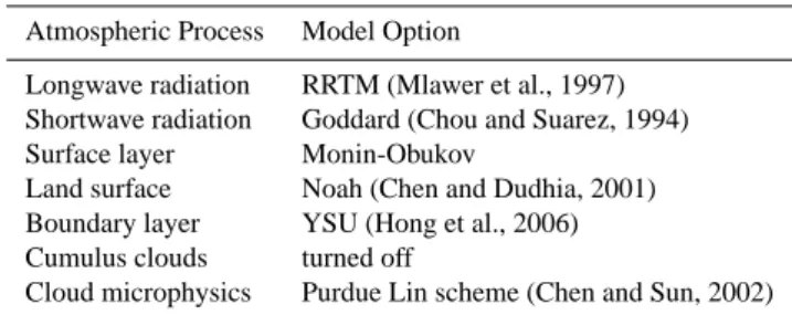
Table 1. Parameterizations employed by WRF in this study.
Atmospheric Process Model Option
Longwave radiation RRTM (Mlawer et al., 1997) Shortwave radiation Goddard (Chou and Suarez, 1994) Surface layer Monin-Obukov
Land surface Noah (Chen and Dudhia, 2001) Boundary layer YSU (Hong et al., 2006) Cumulus clouds turned off
Cloud microphysics Purdue Lin scheme (Chen and Sun, 2002)
March. Two domains were employed: an outer domain en-compassing most of Mexico and the surrounding ocean with a grid spacing of 12 km, and a 205 km×157 km inner do-main encompassing central Mexico with a grid spacing of 3 km. The initial and boundary conditions for WRF were based on the National Center for Environmental Prediction’s Global Forecast System analyses available every six hours. Table 1 lists the specific parameterizations used by WRF in this study.
Four-dimensional data assimilation (4DDA) that em-ployed an observational nudging technique (Liu et al., 2006; Stauffer and Seaman, 1994) was used to constrain the me-teorology during the simulation period. Wind speed and direction data were obtained to heights of approximately 4000 m from radar wind profilers at T0, T1, T2, and Veracruz (∼315 km east of Mexico City). Wind speed, direction, tem-perature, and humidity values were extracted from the 00:00, 06:00, 12:00, and 18:00 UTC soundings at Mexico City, Aca-pulco (∼300 km south of Mexico City) and Veracruz. The spatial influence of the measurements was limited to a hori-zontal distance of 30 km near the surface so that the complex circulations resulting from terrain forcing were not overly smoothed. Because most of the measurements were located between Mexico City and T2, the meteorological conditions were constrained only over a small portion of the modeling domain.
Figure 2 show an example of the measured wind fields at two heights at the T1 site, along with the model values with and without data assimilation. Winds from a south-westerly direction may transport material from the MCMA over T1 and T2, and the figure shows that these conditions are often found at ∼2100 m but less consistently at ∼400 m AGL (above ground level). The wind directions closer to the surface are more variable than higher up, reflecting the strong influence of localized thermal and topographic forc-ing. Throughout the simulation period the model does a gen-erally good job of reproducing the observations even without data assimilation, but there are some improvements when as-similation is carried out, as expected. At the higher eleva-tions the agreement between measured and modeled speeds is somewhat better than at the lower ones. We call attention
33
Fig. 2. Measured (dots) and modeled (lines) wind speeds and
direc-tions at T1. Model values are shown without (red) and with (blue) data assimilation.
to the period of 18–21 March when winds from the south southwest prevailed throughout the lowest 2 km or more. This time period appeared to be particularly favorable for transport of the MCMA plume over T1 and T2 (e.g., Fig. 9 in this paper and trajectories shown in Doran et al. (2007)), and the modeled winds agree especially well with the data. The comparisons between measured and modeled winds at T2 (not shown) gave similar good agreement.
The transport and turbulent mixing of tracers was simu-lated using the FLEXPART Lagrangian particle dispersion model (Stohl, 2005). FLEXPART was originally designed to use meteorological fields produced by global models, but we adapted it to use meteorological fields produced by WRF and to have turbulent mixing consistent with mesoscale applica-tions.
In this study, meteorological fields at 30-min intervals were used to drive FLEXPART. Passive tracer particles were released to mimic the spatially and temporally varying emis-sion rates of black carbon. Three types of sources were defined: 1) anthropogenic black carbon released within the Mexico Valley (MCMA sources), 2) anthropogenic black carbon released outside of the Mexico Valley, and 3) black carbon released from biomass burning sources.
An-34
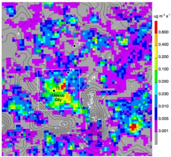
Fig. 3. Map of anthropogenic black carbon emission rates used
for simulations. White dots correspond to biomass burning sources from MODIS during March and the white box outlines the MCMA source region. Black contour intervals are 200 m.
thropogenic emission rates were estimated using the 1999 National Emission Inventory (NEI; http://www.epa.gov/ttn/ chief/net/1999inventory.html). In the NEI inventory, emis-sion ratios of BC/PM2.5 averaged over urban and
subur-ban areas of Phoenix, Houston, and Dallas are given as 0.127, 0.222, and 0.124, respectively, with the high value for Houston perhaps related to the petrochemical facilities concentrated there. The NEI inventory contains emission rates of PM2.5 over Mexico (http://www.epa.gov/ttn/chief/
net/mexico.html) that are not speciated, but an investigation for Mexico City (Miguel Zavala, private communication) has suggested a value of 0.18 for BC/PM2.5 in that region. We
settled on a value for the black carbon released of 0.15 of the total PM2.5mass, which is an intermediate value among
the various estimates we had available. Biomass burning emission rates were derived from MODIS fire count data and vegetation type as described by Wiedinmyer et al. (2006). Biomass burning emission rates varied diurnally with the lowest values around sunrise and peak values during the late afternoon. Figure 3 shows a map of the study area with the anthropogenic emission rates of black carbon for the MCMA and non-MCMA area as well as the locations of biomass burning sites from the MODIS data.
The median ages (from the time of release) of the tracer particles in boxes 5 km on a side at T1 and T2 were com-puted, as were the fractions of the particles in each box originating from each type of source. The output from the model was then used to identify and select periods for anal-ysis, based on factors such as median particle age, fraction of the EC arising from MCMA sources, and transport of the
Fig. 4. (a) Contour plot of particle concentrations at 900 m AGL at 15:30 LST on 20 March, and flight paths of G-1 aircraft over T1 and T2
during the afternoon. (b) Measured CO mixing ratios on the G-1 (blue dots), simulated tracer particle concentrations at the G-1 locations interpolated to the times the G-1 crossed those locations (red dots), and range of simulated particle concentrations at each location during the G-1 flights (gray shading).
MCMA plume between T1 and T2. Subsequent tests with boxes 10 km on a side gave results similar to those with 5 km sides.
3 Model evaluation
3.1 Comparison of tracer particle concentrations with air-craft observations
DOE’s Gulfstream-1 (G-1) aircraft flew a number of mis-sions over the T1 and T2 sites during the course of the exper-iment, and the data from some of those flights can be used to help assess the performance of the model. The top panel of Fig. 4 shows the tracks of one of those flights on the af-ternoon of 20 March overlaid on a contour map of simulated particle concentrations at an elevation of 900 m AGL. Flight tracks at three heights over T1 and T2 are stacked on top of each other in the figure. The bottom panel shows the ob-served CO concentrations (blue dots) that we used as a sur-rogate for black carbon (Baumgardner et al., 2002), which was not measured on the G-1. Results for the three sampling heights over T1 and T2 are shown, with nominal altitudes
of 2070, 1460, and 860 m AGL over T1 and 600, 1210, and 1830 m AGL over T2. The red dots are the model values at the G-1 locations interpolated to the times the G-1 crossed those locations, and the gray shading denotes the range of simulated values at each location during the whole G-1 sam-pling time period. Although all of the details are not repli-cated, the model does a reasonably good job of simulating the position and width of the anthropogenic plume northeast of Mexico City.
3.2 Comparison of tracer particle concentrations with sur-face EC measurements
Figure 5 shows time series of the EC concentrations mea-sured at the T1 site. It also shows the total number of tracer particles in boxes 5 km on a side centered at T1. A lowess filter (Cleveland, 1979) with a ∼6-h smoothing window is drawn through each of the series to highlight the more reg-ular variations of the series, especially the diel variations of EC. The simulated tracer particle counts show temporal vari-ations that are similar to those found for the EC values. The model generally captures the timing of the diel fluctuations
36
Fig. 5. Time series of the EC concentrations measured at the T1
site, and the total number of tracer particles in boxes 5 km on a side centered at T1. The line is a lowess filter through the data. Nighttime periods are indicated by the shaded areas.
but it has more difficulty with the magnitudes of the signal. The largest discrepancies occur on 25 and 26 March with two major peaks in the particle counts; although they correspond to peaks in the EC concentrations, the latter are consider-ably less prominent. We speculate that the observed EC may have been reduced by precipitation scavenging during rainy episodes in the last several days of this period, an effect that is not captured in the numerical simulations.
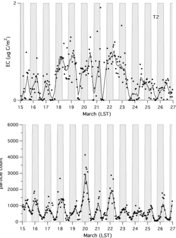
Figure 6 shows the corresponding behavior of EC and tracer particles at T2. The EC variations do not have the same regularity in diel trends as those found at T1, nor do the vari-ations in the particle counts show the same degree of fidelity to the EC variations as was found for T1. The EC concen-trations for 18–23 March are generally higher than for the rest of the period, reflecting the prevalence of favorable wind conditions that bring the MCMA plume and material from biomass burning over T2 during much of that time, and there are major peaks in the tracer particle counts on 18, 20, and 22 March. The particle peaks drop off too quickly, however, so that the broad maximum in the EC concentration time series is not well captured by the particle simulations.
37
Fig. 6. As in Fig. 5 except for the T2 site.
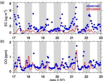
There are a number of factors that may contribute to the poorer performance of the model in simulating EC concen-trations at T2. First, the simulated dispersion over the mod-eling domain is necessarily imperfect. Errors in the sim-ulated wind speeds or directions, the depth of the bound-ary layer, or the representations of the turbulent mixing can all lead to errors in the dispersion patterns. As noted ear-lier, the agreement between measured and modeled speeds is better at higher elevations than closer to the surface, which may account for the better agreement with the G-1 obser-vations shown in Fig. 4. Moreover, the emission invento-ries for MCMA and non-MCMA anthropogenic sources and the biomass burning sources have their own uncertainties, so that the strength, location, and timing of important sources may not be adequately represented. A comparison of the time series of observed values of CO and EC with simu-lated values obtained from the WRF-Chem model (Fast et al., 2006) for T1 is shown in Fig. 7. The model does a rea-sonable job of capturing the temporal variations of the CO and EC but the magnitude of the simulated EC is typically too small. This suggests that there are likely more uncer-tainties in EC emission rates than CO emission rates from anthropogenic and biomass burning sources, because both quantities are equally affected by the predicted meteorology.
38
Fig. 7. Time series of observed (blue dots) and simulated (red lines)
EC and CO concentrations at T1 for the period 17–23 March.
39
Fig. 8. Variation of EC concentrations with CO concentration at T1
for conditions when the MCMA fraction is greater than or equal to 0.55 (black dots) or less than 0.55 (red dots).
In addition, EC concentrations at T2 are generally smaller than at T1 and biomass burning is a more important source of EC (cf. Fig. 9), so that even small errors in the biomass burning inventory can result in considerable uncertainty in calculated EC concentrations at T2. As a result, more care must be taken when analyzing the T2 data compared to that needed for the T1 data.
3.3 Comparisons of EC and CO measurements
In his review of this work, Baumgardner suggested that an examination of the slope of the EC-CO relationship might be able to distinguish occasions when the majority of the EC
40
Fig. 9. Computed median ages of collections of simulated tracer
particles and the computed fractions of the particles at each site that are attributable to MCMA (red lines) and to biomass burning (green lines) sources at T1 (upper two panels) and T2 (lower two panels). The filled areas in the plots of median ages indicate the 25th to 75the percentile range of values. The filled areas in the bottom panel correspond to times identified as transport periods with the MCMA fraction ≥0.4 and the median particle age ≤6 h.
was coming from Mexico City from those when the EC val-ues were heavily influenced by biomass burning. Figure 8 shows such a comparison of measured CO and EC. In the figure the black points correspond to periods when the frac-tion of tracer particles at T1 attributable to MCMA sources was 0.55 or larger, while the red points were obtained when this fraction was less than 0.55. The value of 0.55 was cho-sen because it is the median value of the MCMA fraction for the complete analyzed time series. We are unable to discern any clear separation of the two sets of points in the figure, and we suggest the following reason for the observed scatter. In the emissions inventories available to us, the CO-EC re-lationship varies among different sectors of the city, and the CO-EC relationship for various biomass sources also varies. Thus, while a good CO-EC correlation might be obtained closer to local sources within the city, a downwind site like T1 is influenced by a variety of sources with differing CO-EC slopes. Thus, a clear separation of MCMA-dominated
41
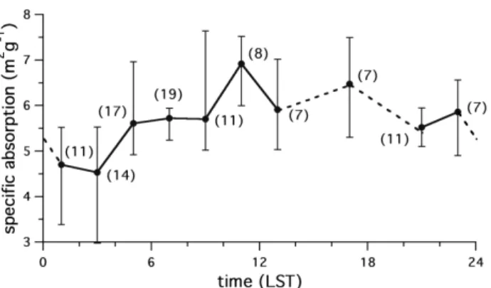
Fig. 10. Variation of median specific absorption (at 870 nm) at T1
with time when MCMA fraction ≥0.5 and median age <12 h. Num-bers in parentheses are the number of samples in each 2-h time bin used to compute the median values. Dashed lines indicate missing values and vertical lines indicate 25th and 75th percentile values.
and biomass burning-dominated periods is less likely to be evident in the CO-EC slopes.
4 Results and discussion
4.1 Particle ages
Figure 9 shows time series of the computed median ages of tracer particles at T1 and T2. Here, age means the time from the emission of the tracer particle until its arrival at one of the two sites. Also shown in the figure are the computed fractions of the particles at each site that are attributable to MCMA and to biomass burning sources. Given the ability of the tracer simulations to mimic the EC concentrations, we can expect the ages and the MCMA and biomass fractions to be reasonably accurate at T1 but subject to more uncer-tainty at T2. Despite this unceruncer-tainty, it is clear that the me-dian ages of the tracer particles at T1 are usually smaller than those at T2, reflecting the proximity of the MCMA to T1 and the dominant role that the MCMA emissions have at the T1 site. For the 15–27 March period at T1, the median ages were small at night ( ∼1–3 h) and increased during the early after-noon (∼11 h). T2 showed similar trends but the median ages ranged between approximately 3 and 14 h.
4.2 Biomass burning
From Fig. 9 it appears that biomass burning occasionally contributed a significant portion of the elemental carbon measured at T1 even thought the primary source of EC was typically the MCMA. At T2 the biomass contribution is more likely to have been the primary one for much of the period. The details of the biomass calculations should also be used with some care, however. In addition to the difficulties as-sociated with simulating the dispersion of EC over the do-main described above, the estimation of black carbon
emis-sions from biomass burning is also uncertain. Wiedinmyer et al. (2006) discuss some of the limitations of the emissions inventory used for this study, and Yokelson et al. (2007) note that MODIS fire count data may substantially underestimate the number of fires in the Mexico City area during the MI-LAGRO campaign. Reid et al. (2005) reviewed sources of uncertainty for biomass burning and summarized the large range of emission factors that have been reported in the lit-erature. That problem is exacerbated by investigators’ use of different procedures for determining OC and EC fractions in samples analyzed by thermal methods, such as those used in this study. In this context Reid et al. conclude that “results must be treated as semi-quantitative, and the best an investi-gator can currently hope for is consistency”. Thus, while the information provided in Fig. 9 provides a sense of the impor-tance of the contributions from biomass burning, we must also expect some uncertainty in estimates of its effect on ei-ther the amount or age of the elemental carbon, especially at T2.
4.3 Variations of αABSat T1
We have calculated values of αABSfor times when the
frac-tion of tracer particles attributable to MCMA sources was equal to or larger than the median MCMA fraction of 0.55, and the median age was 12 h or less at T1. We choose these values to exclude periods when biomass burning may have been the dominant contributor to the observed EC at this site and to focus on more recent rather than aged emissions. Fig-ure 10 shows the variation with hour of the day of the median values of αABSat T1 computed for the period 15–27 March.
Because the distributions of specific absorption and age are skewed and can have some large outliers, we prefer to use median values rather than mean values as a more robust indi-cator of behavior. If fewer than six values were available for a given two-hour block, the median is not displayed. The small sample sizes during the afternoon are attributable in large measure to the limitation we imposed on the median ages of the particles. At night and during the early morning hours, local sources contribute strongly to particle concentrations at T1. In late morning or afternoon, the deepening boundary layer can entrain particles from layers aloft that may origi-nate from more distant or older sources, and the median ages of the particles at T1 increase rapidly. When we eliminate periods strongly affected by these older particles, the sample size is substantially reduced. Although the sample sizes for the remaining cases are not large, some trends do stand out. Values of αABS increase slowly after reaching a minimum
in the early morning hours, and then grow further after sun-rise as the day progresses. The values then decrease quickly in the early evening and somewhat more slowly thereafter. There is considerable variation during the diel cycle, with the maximum median value of αABSabout 50% higher than
the minimum. The range of values and the timing of the min-ima and maxmin-ima differ from those reported by Baumgardner
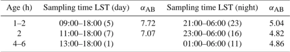
Table 2. Median values of αABS at T1 at 870 nm, in m2g−1, as a function of median tracer particle age, for periods when the MCMA
fraction of the modeled tracer particle concentrations were ≥0.5. Numbers in parentheses following the sampling times are the number of sample hours in that category.
Age (h) Sampling time LST (day) αAB Sampling time LST (night) αAB
1–2 09:00–18:00 (5) 7.72 21:00–06:00 (23) 5.04
2 11:00–18:00 (7) 7.07 23:00–06:00 (16) 4.82
4–6 13:00–18:00 (1) 01:00–06:00 (11) 4.86
et al. (2007), who found that αABS increased only slightly
during the day, with a minimum occurring at approximately 08:00 LST. Our differences in the temporal behavior of αABS
may be related to the relative locations of their and our sam-pling sites. For example, Baumgardner has pointed out in a review of this work that their site was quite close (within 300 m) of a significant source of EC, leaving little time for aerosol growth through diffusion or condensation.
For comparisons with previous measurements we extrap-olated our values of specific absorption from 870 nm to 550 nm using a λ−1 dependence, which increases our val-ues by a factor of 1.58. For all cases our values aver-age about 9.0 m2g−1during the mid-morning hours (08:00– 11:00 LST) at T1. This compares reasonably well with the values of 7.4 to 8.1 m2g−1derived by Barnard et al. (2007) from column measurements with a rotating shadowband ra-diometer in Mexico City in 2003. In contrast, the mea-surements of Baumgardner et al. (2007) gave values of 4.5– 5.0 m2g−1, while a value of 7.0 m2g−1was reported earlier
by Baumgardner et al. (2002). These values are all consis-tent with suggestions by Fuller et al. (1999) that αABS is
not likely to exceed 10 m2g−1except under restrictive con-ditions not met in the MCMA. Specific reasons for the dif-ferences among the various measurements are not known but are probably attributable, at least in part, to the different lo-cations for the measurements. Another possibility is that different measurement techniques contributed to the differ-ences, although Slowik et al. (2007) report good agreement between measurements of black carbon content using a PAS and a Single Particle Soot Photometer, the instrument used by Baumgardner et al. (2007). A number of instrument com-parison studies have been conducted in the past (e.g., Sheri-dan et al., 2005) but have not typically included comparisons between in situ and column measurements of the type de-scribed here. Additional side-by-side comparisons of the var-ious techniques in the field would be useful in the future.
We used the mesoscale model results to estimate ages for the aerosols responsible for the absorption at T1 during both daytime and nighttime. We binned the median ages into bins of 1–2 h, 2–4 h, and 4–6 h, and calculated the median ab-sorption for each bin. We selected the time periods during which measurements were made to ensure that aerosols with ages corresponding to each bin were either always in
sun-light or always in the dark. For example, for aerosols with median ages of 1–2 h, the sampling times for daylight con-ditions were 09:00 to 18:00 LST. If sampling times earlier than 09:00 LST had been used, a 2-h old aerosol would have spent part of its life prior to sunrise. For aerosols in the 2– 4 h bin the beginning sampling time was delayed further until 11:00 LST. The results are shown in Table 2.
The rate of coating of soot and the enhancement of αAB
may be expected to depend on solar radiation and the con-centration of condensable species, and these will both vary with time and location during the daylight hours; at night, coagulation may be the more important process (Riemer at al., 2004). Thus, a simple relationship between soot age and a particular value of αABshould not be expected. From our
data we found that the specific absorption values decreased as the median ages of the particles increased from 1–2 h to 2–4 h, and they did so during both the day and night. There was a negligible subsequent increase in αABS for the 4–6 h
bin at night, but only one case in that age category was found for the day. Because of the small sample sizes and the small differences, none of the daytime or nighttime differences in Table 2 are statistically significant at the 5% level; the dif-ferences between daytime and nighttime values for the cor-responding age bins are significant at the 5% level.
Our results do suggest that soot aging and coating proceed quite rapidly during the day and that any increases in ab-sorption after the first hour or so of the aerosol’s lifetime are small. Conversely, at night photochemical processing is ab-sent, the aging and coating proceed more slowly, and values of αABSare less affected by coating. This is broadly
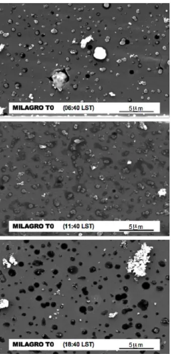
consis-tent with the observations of Johnson et al. (2005) and the modeling work of Riemer et al. (2004) described earlier. Ad-ditional support for this suggestion is provided by electron microscopy analysis of particles collected at the T0, T1 and T2 sites during the 2006 campaign. As an example, Fig. 11 shows a series of scanning electron microscope (SEM) im-ages of particles collected at T0 on 22 March. As indicated by the micrographs, particles in early morning samples are seen as “dry” grey spots with little or no coating. In con-trast, particles collected during the late morning or afternoon hours show clear evidence of organic coating. This coating – apparent in the images as the darker substance surround-ing the grey particles – is likely photo-chemically formed
Fig. 11. SEM images of particles collected at the T0 sampling site
at three times on 22 March. The darker areas around the particles indicate coating of particles by organic material during the daytime.
secondary organic material that condensed on already exist-ing traffic emissions particles (D. Worsnop, private commu-nication). Such behavior was found on numerous days during the MILAGRO campaign at all three sampling sites.
The measured OC/EC ratios at T1 also support this inter-pretation, showing a broad peak in the afternoon and much smaller values at night (Fig. 12). A minimum in the OC/EC ratio occurs in the 06:00–08:00 LST interval. This behavior is consistent with the finding of Baumgardner et al. (2007)
43
Fig. 12. Variation of median OC/EC ratio with time when MCMA
fraction ≥0.55 and median age <12 h at T1. Dashed lines indicate missing values and vertical lines indicate 25th and 75th percentile values.
that the thinnest coating of non-light absorbing material was observed at the time of maximum concentrations of light ab-sorbing carbon around 08:00 LST.
Our observations regarding the variation of αABSwith age
should be treated with some caution. The numbers of sam-ples in each category in the table are not large, especially during daylight hours, and the range of median particle ages that we could analyze was limited. The model results are also subject to uncertainty, as described earlier, and the data themselves have their own sources of potential error (e.g., Watson et al., 2005). Nonetheless we felt it would be inter-esting and potentially useful to present the features shown in Table 2. Our selection of conditions to analyze based on a threshold MCMA fraction of tracer particles ≥0.55 is also somewhat arbitrary. A value of 0.55 for the MCMA frac-tion still allows a considerable influence from other sources such as biomass burning. We have looked at higher thresh-olds but the number of cases available for analysis decreases and the statistical significance also decreases. We also re-laxed the criterion for MCMA fraction to allow more influ-ence from non-MCMA sources. The principal differinflu-ence we found was that as the percentage of the tracer particles at-tributed to biomass burning increased, the median ages of the tracer particles also increased, as was expected. In prin-ciple we could use model results to sort out the relative ef-fects of particle age and MCMA or biomass burning fraction on αABS, but in practice our number of samples becomes too
small to allow unambiguous results to be obtained. 4.4 Change of αABSbetween T1 and T2
One of the objectives of the T1-T2 campaign was to exam-ine changes in αABS as the Mexico City urban plume was
advected first over T1 and then over T2. The expectation was that if aerosols aged and became coated en route from T1 to T2, then those processes would result in measurable
differences in αABS between the two sites. Initial analyses
(Doran et al., 2007; Doran, 2007) provided some evidence suggesting such changes had been observed but the statis-tical significance of the differences was not strong. More-over, possible influences of biomass burning were recog-nized as a complicating factor that needed to be considered in greater detail, and for this paper we hoped that the results of our mesoscale modeling could provide additional insight. In light of the uncertainties in the modeling and measure-ments described earlier, we chose to restrict comparisons of the specific absorption of elemental carbon at the T1 and T2 sites to transport periods when the urban plume from the MCMA region was likely to have been a major contributor to the EC concentrations at both T1 and T2. These periods would be characterized in Fig. 9 by relatively high fractions of the tracer particles from MCMA sources and by relatively small values of the median ages of the ensemble of particles at each site. We also needed to strike a balance between the highly restrictive conditions for which the simulated biomass burning contributions are likely to have been very small (e.g., less than 20% of the tracer particles at a site) and having enough measurements of specific absorption to allow for rea-sonable size samples for comparison. In practice we settled on two criteria for identifying transport periods: 1) the com-puted MCMA fraction of the tracer particles at T2 was 0.4 or higher, and 2) the simulated median transport time at T2 was 6 h or less. These periods are indicated by the filled-in por-tions of the MCMA curve in the bottom panel of Fig. 9. Most of these cases are found around the period 18–21 March, and a comparison with the data presented in Fig. 2 shows that this period corresponded to a time interval during which both near-surface winds and winds aloft blew from the south southwest. We have also used a 10 km×10 km box surround-ing T2 to calculate the MCMA fraction and median particle ages, and we found that the periods identified as favorable for T1-T2 comparisons are virtually the same as those found using the 5 km×5 km box.
The criteria used above to select “transport periods” are considerably more restrictive than the preliminary criteria used in our previous study (Doran et al., 2007), which were based on estimates of trajectories from the T1 profiler without regard to possible influences from biomass burn-ing sources. In addition, for this study we further limited our analysis to times when specific absorption measurements were available at both T1 and T2 and the computed age of the particles at T2 was greater than that at T1. As a result the sample population has been reduced by more than a fac-tor of two from our earlier analysis (to 23 cases), primarily because of the exclusion of periods with large contributions from biomass burning.
During these more restricted transport periods the me-dian specific absorption of EC at 870 nm at T1 and T2 was 5.72 and 5.97 m2g−1, respectively, but a Mann-Whitney test shows that the difference in the median values of αABS at
T1 and T2 was significant only around the 20% level. If we
relax the 6-h restriction for the median age of the particles at T2 to 12 h, there is no significant difference in the median specific absorption at the two sites even at the 50% level. It is interesting to note that for all other times that do not include transport cases, the median values of αABSdecrease between
T1 and T2, from 5.61 to 5.41 m2g−1, but this difference is again not significantly different from zero at the 50% level.
An examination of individual cases shows that the differ-ences in the calculated median ages of the tracer particles between T1 and T2 for transport conditions ranged approxi-mately from 1 to 4 h. Given the results from T1 shown ear-lier on the variation of αABS with age, it is unclear why the
specific absorption would increase during the relatively brief travel times between T1 and T2.
4.5 Future studies
At this point it is difficult to judge the importance of the small differences in αABS between T1 and T2 without a
measure-ment campaign of longer duration and perhaps a selection of locations with greater separation to provide additional data. For example, conditions favorable for transport between T1 and T2 also occurred on 9–11 March, before the full suite of instruments was operational at the two sites. Future cam-paigns lasting for two months or more would increase the number of cases with conditions favorable for analysis. The use of a mesoscale model with data assimilation to help an-alyze the results, as described here, would clearly be a valu-able component of any such study.
Further evidence of the relative impacts of anthropogenic and biomass burning on particulates observed downwind from Mexico City should come from several aerosol mass spectrometers (AMS) that were deployed at ground sites (T0, T1, and mobile platforms) and on aircraft (G-1 and C-130). Recently developed analysis methods for AMS organic spectra can separate organic mass into hydrocarbon-like (re-ferred to as HOA) and oxygenated components (re(re-ferred to as OOA). Zhang et al. (2005) and Volkamer et al. (2006) show that HOA and OOA correspond to primary and secondary organics, respectively. This analysis technique has been ex-tended to include a category resulting from biomass burning (referred to as BBOA). The time variations of HOA, OOA, and BBOA at the surface sites and on the aircraft should allow identification of anthropogenic and biomass contribu-tions to aerosols at T1 and T2 as well as information on how much coating of the aerosols occurred from secondary pro-cesses. The data on HOA, OOA, and BBOA components of the organic particulates are not yet available for this paper, but coupling that information with our analyses in the future would clearly be worthwhile.
5 Summary and conclusions
We have used the WRF model, along with 4DDA, to sim-ulate the local, regional, and synoptic meteorological condi-tions during the MILAGRO field campaign. The meteorolog-ical fields were used to drive a Lagrangian dispersion model, with tracer particles released at rates based on emission in-ventories for black carbon from anthropogenic sources and biomass burning. The results were used to identify periods when relatively fresh emissions from the MCMA were the primary contributors of EC at T1. They were then used to help examine the changes of the specific absorption, αABS,
with time of day and with time after release. Coating of EC, with a consequent increase in αABS, appears to be limited
during night. In contrast, coating proceeds rapidly during the day, with peak values of αABS occurring in mid-afternoon.
This interpretation is supported by SEM images of aerosols collected at the sampling sites and by measured OC/EC ra-tios at the T1 site.
Although αABS increases during the day, strong evidence
for increases of αABS with particle age for median aerosol
ages up to 6 h was not found. There was a small increase in
αABSbetween the T1 and T2 sites on days with conditions fa-vorable for transporting the MCMA plume over the two sites, but the statistical significance of this result was marginal. For non-transport conditions the median values of αABSat the T1
and T2 sites were essentially the same. Additional measure-ments taken over more extended time periods, perhaps with more widely separated sampling sites, would be valuable. Acknowledgements. This research was supported by the Office of
Science (BER), U.S. Department of Energy, under the auspices of the Atmospheric Science Program, under Contract DE-AC05-76RL01830 at the Pacific Northwest National Laboratory. Pacific Northwest National Laboratory is operated for the U.S. DOE by Battelle Memorial Institute. We thank P. Arnott and G. Paredes-Miranda of the Desert Research Institute for their PAS data, L. Kleinman of Brookhaven National Laboratory for the CO data from the G-1, and G. Huey of Georgia Institute of Technology for the CO data at T1. Finally, we thank D. Baumgardner for suggesting a possible source of the different values of αABSin his
and our studies. Edited by: L. Molina
References
Andreae, M. O. and Gelencs´er, A.: Black carbon or brown carbon? The nature of light-absorbing aerosols, Atmos. Chem. Phys., 6, 3131–3148, 2006,
http://www.atmos-chem-phys.net/6/3131/2006/.
Arnott, W. P., Moosm¨uller, H., Rogers, C. F., Jin, T., and Bruch, R.: Photoacoustic Spectrometer for Measuring Light Absorption by Aerosols: Instrument Description, Atmos. Environ., 33, 2845– 2852, 1999.
Arnott, W. P., Moosm¨uller, H., Sheridan, P. J., Ogren, J. A., Raspert, R., Slaton, W. V., Hand, J. L., Kreidenweis, S. M.,
and Collett Jr., J. L.: Photoacoustic and filter-based ambient aerosol light absorption measurements: instrument comparisons and the role of relative humidity, J. Geophys. Res., 108, 4034, doi:10.1029/2002JD002165, 2003.
Barnard, J. C., Kassianov, E. I., Ackerman, T. P., Johnson, K., Zu-beri, B., Molina, L. T., and Molina, M. J.: Estimation of a “radia-tively correct” black carbon specific absorption during the Mex-ico City Metropolitan Area (MCMA) 2003 field campaign, At-mos. Chem. Phys., 7, 1645–1655, 2007,
http://www.atmos-chem-phys.net/7/1645/2007/.
Baumgardner, D., Raga, G. B., Kok, G., Ogren, J., Rosas, I., B´aez, A., and Novakov, T.: On the evolution of aerosol properties at a mountain site above Mexico City, J. Geophys. Res., 105, 22 243– 22 253, 2000.
Baumgardner, D., Raga, G., Peralta, O., Rosas, I., Castro, T., Kuhlbusch, T., John, A., and Petzold, A.: Diagnos-ing black carbon trends in large urban areas usDiagnos-ing carbon monoxide measurements, J. Geophys. Res., 107(D21), 8342, 10.1029/2001JD000626, 2002.
Baumgardner, D., Kok, G. L., and Raga, G. B.: On the diurnal variability of particle properties related to light absorbing carbon in Mexico City, Atmos. Chem. Phys., 7, 2517–226, 2007, http://www.atmos-chem-phys.net/7/2517/2007/.
Birch, M. E. and Cary, R. A.: Elemental carbon-based method for monitoring occupational exposures to particulate diesel exhaust, Aerosol Sci. Technol., 25, 221–241, 1996.
Bond, T. C. and Bergstrom, R. W.: Light absorption by carbona-ceous particles: an investigative review, Aerosol Sci. Technol., 40, 27–67, doi:10.1080/02786820500421521, 2006.
Bond, T. C., Habib, G., and Bergstrom, R. W.: Limitations in the enhancement of visible light absorption due to mixing state, J. Geophys. Res., 111, D20211, doi:10.1029/2006JD007315, 2006. Burtscher, H., Leonard, A., Steiner, D., Baltensperger, U., and We-ber, A.: Aging of combustion particles in the atmosphere – re-sults from a field study in Z¨urich, Water, Air, Soil Poll., 68, 137– 147,1993.
Chen, F. and Dudhia, J.: Coupling an advanced
land-surface/hydrology model with the Penn State / NCAR MM5 modeling system. Part I: Model description and implementation, Mon. Weather Rev., 129, 569–585, 2001.
Chen S.-H. and W.-Y. Sun: A one-dimensional time dependent cloud model, J. Meteor. Soc Japan, 80, 99–118, 2002.
Chou, M.-D. and Suarez, M. J.: An efficient thermal infrared ra-diation parameterization for use in general circulation models, NASA Tech. Memo. 104606, 3, 85 pp., 1994.
Cleveland, W. S.: Robust locally weighted regression and smooth-ing scatterplots, J. Amer. Statist. Assoc., 74, 829–836, 1979. Croft, B., Lohmann, U., and von Salzen, K: Direct Aerosol Forcing:
Calculation from Observables and Sensitivities to Inputs, Atmos. Chem. Phys., 5, 1931–1949, 2005,
http://www.atmos-chem-phys.net/5/1931/2005/.
Doran, J. C., Barnard, J. C., Arnott, W. P., Cary, R., Coulter, R. L., Fast, J. D., Kassianov, E. I., Kleinman, L. I., Laulainen, N. S., Martin, T. J., Paredes-Miranda, G. L., Pekour, M. S., Shaw, W. J., Smith, D. F., Springston, S. R., and Yu, X. Y.: The T1-T2 Study: Evolution of Aerosol Properties Downwind of Mexico City, Atmos. Chem. Phys., 7, 1585–1598, 2007,
http://www.atmos-chem-phys.net/7/1585/2007/.
aerosol properties downwind of Mexico City” published in At-mos. Chem. Phys., 7, 1585–1598, 2007, AtAt-mos. Chem. Phys., 7, 2197–2198, 2007,
http://www.atmos-chem-phys.net/7/2197/2007/.
Fast, J. D, Gustafson Jr., W. I., Easter, R. C., Zaveri, R. A., Barnard, J. C., Chapman, E. G., and Grell, G. A.: Evolution of ozone, particulates, and aerosol direct forcing in an urban area using a new fully-coupled meteorology, chemistry, and aerosol model, J. Geophys. Res., 111, doi:10.1029/2005JD006721, 2006. Fuller, K. A., Malm, W. C., and Kreidenweis, S. M.: Effects of
mix-ing on extinction by carbonaceous particles, J. Geophys., Res., 104, 15 941–15 954, 1999.
Hong, S.-Y., Noh, Y., and Dudhia, J.: A new vertical diffusion pack-age with an explicit treatment of entrainment processes, Mon. Weather Rev., 134, 2318–2341, 2006.
Jacobson, M. Z.: Isolating nitrated and aromatic aerosols and ni-trated aromatic gases as sources of ultraviolet light absorption, J. Geophys. Res.-A, 104(D3), 3527–3542, 1999.
Jacobson, M. Z. and Seinfeld, J. H.: Evolution of nanoparticle size and mixing state near the point of emission, Atmos. Environ., 38, 1839–1850, 2004.
Johnson, K. S., Zuberi, B., Molina, L. T., Molina, M. J., Iedema, M. J., Cowin, J. P., Gaspar, D. J., Wang, C., and Laskin, A.: Processing of soot in an urban environment: case study from the Mexico City Metropolitan Area, Atmos. Chem. Phys., 5, 3033– 3043, 2005,
http://www.atmos-chem-phys.net/5/3033/2005/.
Kirchstetter, T. W., Novakov, T., and Hobbs, P. V.: Evidence that the spectral dependence of light absorption by aerosols is af-fected by organic carbon, J. Geophys. Res.-A, 109, D21208, doi:10.1029/2004JD004999, 2004.
Liu, Y., Bourgeois, A., Warner, T., Swerdlin, S., and Hacker, J.: Implementation of observation-nudging based on FDDA into WRF for supporting AFEC test operations, 6th WRF Confer-ence, NCAR, Boulder, CO, 10.7, 2006.
Mallet, M., Roger, J. C., Despiau, J. P., and Dubovik, O.: A study of the mixing state of black carbon in urban zone, J. Geophys. Res., 109, D04202, doi:10.1029/2003JD003940, 2004.
Mann, H. B. and Whitney, D. R.: On a test of whether one of two random variables is stochastically larger than the other, Ann. Math. Stat., 18, 50–60, 1947.
Mlawer, E. J., Taubman, S. J., Brown, P. D., Iacono, M. J., and Clough, S. A.: Radiative transfer for inhomogeneous atmo-sphere: RRTM, a validated correlated-k model for the longwave, J. Geophys. Res., 102, 16 663–16 682, 1997.
Moteki, N., Kondo, Y., Miyazaki, Y., Takegawa, N., Komazaki, Y., Kurata, G., Shirai, T., Blake, D. R., Miyakawa, T., and Koike, M.: Evolution of mixing state of black carbon particles: Aircraft measurements over the western Pacific in March 2004, Geophys. Res. Lett., 34, L11803, doi:10.1029/2006GL028943, 2007. Reid, J. S., Koppmann, R., Eck, T. F., and Eleuterio, D. P.: A review
of biomass burning emissions part II: intensive physical proper-ties of biomass burning particles, Atmos. Chem. Phys., 5, 799– 825, 2005,
http://www.atmos-chem-phys.net/5/799/2005/.
Riemer, N., Vogel, H., and Vogel, B.: Soot aging time scales in polluted regions during day and night, Atmos. Chem. Phys., 4, 1885–1893, 2004,
http://www.atmos-chem-phys.net/4/1885/2004/.
Sato, M., Hansen, J., Koch, D., Lacis, A., Ruedy, R., Dubovik, O., Holben, B., Chin, M., and Novakov, T.: Global atmospheric black carbon inferred from AERONET, Proc. Natl. Acad. Sci., 100, 6319–6324, 2003.
Sheridan, P. J., Arnott, W. P., Ogren, J. A., Anderson, B. E., Atkin-son, D. B., Covert, D. S., Moosmuller, H., Petzold, A., Schmid, B., Strawa, A. W., Varma, R., and Virkkula, A.: The Reno aerosol optics study: An evaluation of aerosol absorption mea-surement methods, Aerosol Sci. Technol., 39, 1–16, 2005. Skamarock, W. C., Klemp, J. B., Dudhia, J., Gill, D. O., Barker, D.
M., Wang, W., and Powers, J. G.: A description of the advanced research WRF version 2. NCAR Technical Note, NCAR/TN-486+STR, 88 pp., 2005.
Slowik, J. G., Cross, E. S., Han, J.-H., Davidovits, P., Onasch, T. B., Jayne, J. T., Williams, L. R., Canagaratna, M. R., Worsnop, D. R., Chakrabarty, R. K., Moosm¨uller, H., Arnott, W. P., Schwarz, J. P., Gao, R.-S., Fahey, D. W., Kok, G. L., and Petzold, A.: An Inter-Comparison of Instruments Measuring Black Carbon Content of Soot Particles, Aerosol Sci. Technol., 41, 3, 295–314, 2007.
Sokolik, I. N. and Toon, O. B.: Incorporation of mineralogical com-position of aerosols into models of radiative properties of min-eral aerosol from the UV to IR wavelengths, J. Geophys. Res.-A, 104(D8), 9423–9444, 1999.
Stauffer, D. R. and Seaman, N.: Multiscale four-dimensional data assimilation, J. Appl. Meteor., 33, 415–434, 1994.
Stohl, A., Forster, C., Frank, A., Seibert, P., and Wotawa, G.: Tech-nical note: The Lagrangian particle dispersion model FLEX-PART version 6.2, Atmos. Chem. Phys., 5, 2461–2474, 2005, http://www.atmos-chem-phys.net/5/2461/2005/.
Volkamer, R., Jimenez, J. L., San Martini, F., Dzepina, K., Zhang, Q., Salcedo, D., Molina, L. T., Worsnop, D. R., and Molina, M. J.: Secondary organic aerosol formation from anthropogenic air pollution: Rapid and higher than expected, Geophys. Res. Lett., 33, L17811, doi:10.1029/2006GL026899, 2006.
Watson, J. G., Chow, J. C., Antony Chen, L.-W.: Summary of or-ganic and elemental carbon/black carbon analysis methods and intercomparisons, Aerosol Air Qual. Res., 5, 65–102, 2005. Wiedinmyer, C., Quayle, B., Geron, C., Beloe, A., McKenzie, D.,
Zhang, X., O’Neill, S., and Wynne, K. K.: Estimating emissions from fires in North America for air quality modeling, Atmos. Environ., 40, 3419–3432 2006.
Yokelson, R. J., Urbanski, S. P., Atlas, E. L., Toohey, D. W., Al-varado, E. C., Crounse, J. D., Wennberg, P. O., Fisher, M. E., Wold, C. E., Campos, T. L., Adachi, K., Buseck, P. R., and Hao, W. M.: Emissions from forest fires near Mexico City, Atmos. Chem. Phys., 7, 5569–5584, 2007,
http://www.atmos-chem-phys.net/7/5569/2007/.
Zhang, Q., Worsnop, D. R., Canagaratna, M. R., and Jimenez, J. L.: Hydrocarbon-like and oxygenated organic aerosols in Pittsburgh: Insights into sources and processes of organic aerosols, Atmos. Chem. Phys., 5, 3289–3311, 2005,