S1
Supporting Information
Particle Size Distributions for Cellulose Nanocrystals Measured by
Transmission Electron Microscopy: An Interlaboratory Comparison
Juris Meija,1 Michael Bushell,1 Martin Couillard,1 Stephanie Beck,2 John Bonevich,3 Kai Cui,4 Johan Foster,5 John Will,5 Douglas Fox,6 Whirang Cho,6 Markus Heidelmann,7 Byong Chon Park,8 Yun Chang Park,9 Lingling Ren,10 Li Xu,10 Aleksandr B. Stefaniak,11 Alycia K. Knepp,11
Ralf Theissmann,12 Horst Purwin,12 Ziqiu Wang,13 Natalia de Val,13 Linda J. Johnston1
1 National Research Council Canada, Ottawa, ON K1A 0R6 Canada 2 FPInnovations, Pointe-Claire, QC H9R 3J9 Canada
3 Materials Science and Engineering Division, National Institute of Standards and Technology, Gaithersburg, MD 20899 USA
4 National Research Council Canada, Nanotechnology Research Centre, Edmonton, AB T6G 2M9, Canada 5 Department of Materials Science and Engineering, Virginia Tech, Blacksburg, VA 24061 USA; Chemical and Biological Engineering, The University of British Columbia, Vancouver, BC V6T 1Z3 Canada 6 Department of Chemistry, American University, Washington DC 20016 USA
7 Interdisciplinary Center for Analytics on the Nanoscale, University of Duisburg-Essen, 47057 Duisburg, Germany
8 Center for Nanocharacterization, Korea Research Institute of Standards and Science, Daejeon 34113, Republic of Korea
9 Division of Measurement & Analysis, National Nanofab Center, Daejeon 34141, Republic of Korea 10 National Institute of Metrology, Chaoyang District, Beijing, China, 100029
11 National Institute for Occupational Safety and Health, Morgantown, WV 26505 USA 12 KRONOS INTERNATIONAL Inc., Peschstrasse 5, 51373 Leverkusen, Germany
13 Electron Microscopy Laboratory, National Cancer Institute, Center for Cancer Research, Leidos Biomedical Research, Frederick National Laboratory, Frederick, MD 21702 USA
Table of Contents
Experimental Section page S2 Figure S1, Table S1 page S3 Figure S2, Figure S3 page S4
Figure S4 page S5
Table S2, Figure S5 page S6 Figures S6, S7, S8, S9 pages S7-S10
Figure S7 page S8
Figure S8 page S9
S2
Experimental
Sample preparation. An NRC certified reference material, CNCD-1, was dispersed to give a
suspension with 2 % CNC mass fraction that was sonicated (5 kJ/g), diluted to 0.025 % with deionized water (18.2 MΩ·cm), and vortex-mixed for 5 s. A carbon-coated copper grid was plasma-exposed using a shielded holder on a Fischione plasma cleaner (Nanoclean 1070, 25 %/ 75 % O2-Ar plasma for 2 min at ≈40 W). The amount of CNC suspension, incubation, and wash
time and conditions and staining procedure were optimized to minimize agglomerated CNCs while ensuring a reasonable number of individual CNCs in the field of view. For the optimized procedure, 10 µL of the 0.025 % CNC suspension was deposited, left for 4 min and wicked with a piece of filter paper. The sample was washed by adding one drop of deionized water to the grid and wicking with filter paper. Finally, the sample was stained by depositing 10 µL of a filtered (0.22 µm PVDF) 2 % by mass uranyl acetate solution on the grid for 4 min. The grid was then immersed in deionized water, removed and allowed to completely dry in air for 1 h to 2 h. Despite optimization, samples typically showed significant heterogeneity in both stain and CNC density, both between samples and across different regions of the same sample.
Image analysis protocol. A custom ImageJ macro was used for the ILC. The macro allows for
automatic sequential opening of a set of images and manual measurement of appropriate length and width cross sections and saves the data and annotated images with the line profiles for analyzed CNCs. All individual CNCs in each image were to be analyzed using the following guidelines. The length is measured as the longest distance from one end of the CNC to the other and the width is measured perpendicular to the long axis at the widest part of the CNC. Note that some of the individual particles have an irregular shape, but should still be included in the analysis, unless one can clearly detect the presence of two separate particles. The following particles should not be analyzed: (1) agglomerated CNCs; (2) CNCs that are obstructed by a scale bar, imaging artifact or sample contamination; (3) CNCs that lack adequate contrast for
identification of the edges; and (4) CNCs that touch the edge of the image. Adjacent (touching) CNCs may be analyzed if the contrast is sufficient to distinguish the individual particles. Participants were requested to return the original image files and the corresponding files with analyzed particles numbered, and to complete an Excel template with length, width and aspect ratio data, image acquisition and analysis parameters and histograms of the data.
S3
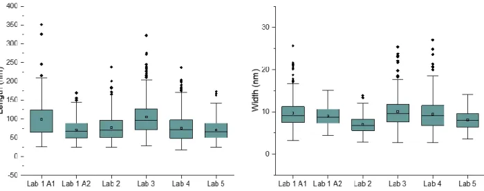
Figure S1. Plots illustrating variability in data received from the image analysis tests. The
bottom and top of the colored boxes represent the 25th and 75th percentiles; the mean and median
are shown as an open square and solid line, respectively; the vertical bars are 1.5 times the interquartile range, with data points that fall outside this range shown as filled diamonds.
Table S1. Summary of results from tests of the image analysis protocol.
Lab1 n
Length, nm Width, nm
Mean (SE)2 Std dev median Mean (SE) Std dev median
Lab 1, analyst 1 (A1) 284 98.6 (2.8) 47.2 89.3 9.8 (0.20) 3.4 9.1 Lab 1, analyst 2 (A2) 128 71.0 (2.6) 29.1 66.9 9.4 (0.22) 5.0 8.7 Lab 2 244 77.1 (2.3) 35.8 70.7 7.0 (0.14) 2.1 6.8 Lab 3 370 105.2 (2.5) 47.4 95.9 10.0 (0.18) 3.4 9.6 Lab 4 442 76.3 (1.8) 37.0 72.3 9.5 (0.18) 3.8 9.2 Lab 5 216 70.7 (1.9) 28.1 66.1 8.1 (0.16) 2.3 8.0
1 Of the 15 possible pairs of laboratories only 2 pairs for each of length and width are not
significantly different, based on the Kolmogorov-Smirnov test: Length, lab 2/lab 4 and lab 2/lab 5; Width, lab 1 A2/lab 3 and lab1 A2/lab 1 A1.
S4
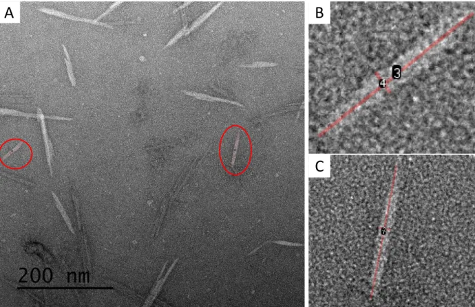
Figure S2. TEM image (A) with expanded views (B, C) showing the size analysis for 2
particles.
Figure S3. TEM image (A) and expanded views of four individual CNCs that are suitable for size
analysis.
A
B
S5
Figure S4. TEM images showing particles that should not be analyzed: (A) aggregated CNCs,
(B) two CNCs, (C) aggregated CNCs, (D) irregular feature that may indicate aggregation, (E) two CNCs arranged end to end, (F) scale bar interference.
A B C
S6
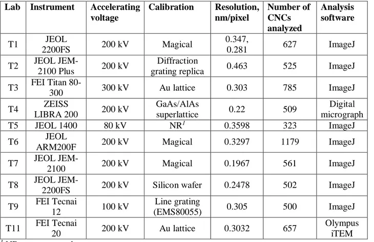
Table S2. Summary of TEM instruments, calibration, operating conditions, and analysis
software as reported by each participating laboratory.
Lab Instrument Accelerating
voltage Calibration Resolution, nm/pixel Number of CNCs analyzed Analysis software T1 JEOL 2200FS 200 kV Magical 0.347, 0.281 627 ImageJ T2 JEOL JEM-2100 Plus 200 kV Diffraction
grating replica 0.463 525 ImageJ T3 FEI Titan 80-300 300 kV Au lattice 0.303 785 ImageJ T4 ZEISS LIBRA 200 200 kV GaAs/AlAs superlattice 0.22 509 Digital micrograph T5 JEOL 1400 80 kV NR1 0.3598 323 ImageJ T6 JEOL
ARM200F 200 kV Magical 0.3297 1179 ImageJ T7 JEOL
JEM-2100 200 kV Magical 0.1967 561 ImageJ T8 JEOL
JEM-2200FS 200 kV Silicon wafer 0.2478 502 ImageJ T9 FEI Tecnai 12 100 kV Line grating (EMS80055) 0.305 500 ImageJ T11 FEI Tecnai 20 200 kV Au lattice 0.3032 657 Olympus iTEM 1 NR = not reported
Figure S5. Box plots of length and width data from each participating laboratory. The colored
boxes show the 25 %, 50 % (median), and 75 % quantiles and the mean is shown as an open square. The vertical bars are 1.5 times the interquartile range, with points that fall outside this range shown as filled diamonds.
S7
Figure S6. Histograms of TEM length data from each laboratory with the skew normal fits
shown as orange lines.
S8
Figure S7. Histograms of TEM width data from each laboratory with the skew normal fits
shown as orange lines.
S9
Figure S8. Histograms of TEM aspect ratio data from each laboratory with the skew normal fits shown as
orange lines.
S10
Figure S9. Plots of cumulative mean as a function of number of analyzed CNCs for length and
width data sets for representative laboratories. The pixel size is 0.46 nm for T2, ~ 0.3 nm for T3 and T6 and ~0.2 nm for T7 (see Table S1). Note that the y-axis covers 15 nm and 1.2 for length and width, respectively, but the plot origin is shifted to fit the data set.