HAL Id: hal-00296075
https://hal.archives-ouvertes.fr/hal-00296075
Submitted on 14 Nov 2006
HAL is a multi-disciplinary open access
archive for the deposit and dissemination of
sci-entific research documents, whether they are
pub-lished or not. The documents may come from
teaching and research institutions in France or
abroad, or from public or private research centers.
L’archive ouverte pluridisciplinaire HAL, est
destinée au dépôt et à la diffusion de documents
scientifiques de niveau recherche, publiés ou non,
émanant des établissements d’enseignement et de
recherche français ou étrangers, des laboratoires
publics ou privés.
atmosphere
K. Kourtidis, I. Kioutsioukis, D. F. Mcginnis, S. Rapsomanikis
To cite this version:
K. Kourtidis, I. Kioutsioukis, D. F. Mcginnis, S. Rapsomanikis. Effects of methane outgassing on the
Black Sea atmosphere. Atmospheric Chemistry and Physics, European Geosciences Union, 2006, 6
(12), pp.5173-5182. �hal-00296075�
Atmos. Chem. Phys., 6, 5173–5182, 2006 www.atmos-chem-phys.net/6/5173/2006/ © Author(s) 2006. This work is licensed under a Creative Commons License.
Atmospheric
Chemistry
and Physics
Effects of methane outgassing on the Black Sea atmosphere
K. Kourtidis1, I. Kioutsioukis1, D. F. McGinnis2, and S. Rapsomanikis1
1Laboratory of Atmospheric Pollution and Pollution Control Engineering of Atmospheric Pollutants, Dept. of Environmental
Engineering, Democritus University of Thrace, P.O. Box 447, 67100 Xanthi, Greece
2Surface Waters – Research and Management, Swiss Federal Institute of Aquatic Science and Technology, Eawag, 6047
Kastanienbaum, Switzerland
Received: 7 February 2006 – Published in Atmos. Chem. Phys. Discuss.: 9 May 2006 Revised: 25 September 2006 – Accepted: 6 November 2006 – Published: 14 November 2006
Abstract. Methane in air and seawater was measured in
the Eastern Black Sea during the 10–18 December 1999
BIGBLACK project cruise. The measurements allowed
for the calculation of supersaturation ratios and methane
fluxes across the air-sea interface. CH4 mixing ratios in
air were generally in the 1.8–2.0 ppmv range, while sur-face (4 m depth) seawater concentrations varied from 4 to 93 ppmv. Above active seep areas, the water was supersat-urated to around 500% with respect to the overlying atmo-sphere. Accordingly, flux densities varied greatly and were
up to 3300 umol m−2day−1. In the Sevastopol harbour,
su-persaturations up to around 3000%, similar to those at the Danube Delta, were observed, while in the Istanbul harbour supersaturations could not be determined because the very high values of water concentrations led to detector satura-tion. Simple modelling shows that the observed fluxes do not have any substantial impact on the methane content of the Black Sea atmosphere, as they would only raise its con-centrations by less than 50 ppt. On the other hand, calcula-tions performed as part of the CRIMEA project show that mud volcano eruptions could episodically raise the methane concentrations well above their regional background for sev-eral tens of kilometres downwind. These calculations, which also apply to mud volcano eruptions elsewhere on the globe, indicate that the spatial extend and the magnitude of the at-mospheric perturbation is such that its observation might lie within the capabilities of existing satellite instrumentation such as SCIAMACHY on ENVISAT.
Correspondence to:K. Kourtidis
(kourtidi@env.duth.gr)
1 Introduction
Methane is an important greenhouse gas and a precursor of tropospheric ozone (e.g. IPCC, 2001; Lelieveld et al., 1993, 1998). It is produced in a variety of thermogenic and bi-ological methanogenic processes, some of which occur on geologic time scales, while others on much shorter ones. As a result of these processes, large variations of the atmo-spheric methane abundance might be expected, especially if large reservoirs become unstable. Such reservoirs include methane hydrates (e.g. Kvenvolden, 1993). Another impor-tant pathway for degassing buried sediments appears to be episodic mud volcano eruptions (e.g. Dimitrov, 2002; Kopf, 2002) and continuous seepage over wide areas as well as over localised gas vents (e.g. Etiope and Klusman, 2002). Under-water seepages have been investigated by many authors in various parts of the world (e.g. Judd et al., 1997; Hornafius et al., 1999; Clark et al., 2000; Klusman et al., 2000), and have been found to result in elevated methane concentrations in the surface waters overlying these seeps (e.g. Cynar and Yayanos, 1992; Ward, 1992).
The Black Sea has received attention as a target of in-vestigations on methane because of the large amounts of methane trapped in the anaerobic sediments and the hydrates present underneath these sediments. Under normal condi-tions, methane is vented from the sediments to the overly-ing water through seeps; some of this methane reaches the water-air interfaced unoxidised and subsequently escapes to the atmosphere, although most of it is consumed from bacte-rial activity within the water column (e.g. Durisch-Kaiser et al., 2005).
Some investigations of the methane flux from the Black Sea to the atmosphere have already been
car-ried out (Amouroux et al., 2002; Schmale et al.,
2005), yielding flux densities generally between 0.19–
0.77 nmol m−2s−1 (16–66 umol m−2day−1), while above
active seeps these might increase to 0.96–2.32 nmol m−2s−1
(83–200 umol m−2day−1) and above river plumes they
might increase even further, up to 5.44 nmol m−2s−1
(470 umol m−2day−1).
To derive these fluxes, Amouroux et al. (2002) and Schmale et al. (2005) used the Liss and Merlivat (1986) and the Wanninkhof (1992) parameterisations of the dependency of the transfer velocity k on wind speed u, hereafter referred to as LM86 and W92, respectively. Both parameterisations are quadratic or near-quadratic; W92, for example,
parame-terises k as a function of u as k=0.31u210(Sc/660)−0.5, where
Scis the Schmidt number of CO2in seawater, 660 is the Sc
for CO2in seawater at 20◦C and u10is the wind speed
cor-rected to 10 m height under neutral conditions.
Recent work, based to a large extent on measurements per-formed during the GasEx-1998 field experiments (McGillis et al., 2004), has resulted in other, cubic parameterisations, which yield better fits to the data (e.g. Hare et al., 2004 and references therein). Wanninkhof and McGillis (1999), using recent laboratory and field studies, proposed a cubic relationship between air-sea gas exchange and wind speed,
k660=0.028u310, or k=0.0283u310(Sc/660)−0.5), which,
com-pared with previous calculations using the W92 parameter-isation, resulted in a significant increase of the calculated
oceanic global annual CO2 uptake. Fairall et al. (2000)
reviewed the theoretical basis of various parameterisation schemes for bulk-to-bulk gas transfer. Since then, McGillis
et al. (2001) used eddy accumulation for CO2 to
deter-mine k and showed that k can be described in their study
as k660=3.3+0.026u310, where k660 is the k normalised to
Sc of 660 cm h−1 (which equals the Sc for CO2 in
seawa-ter at 20◦C). Other recent work used measurements of dual
tracers during the Southern Ocean Iron Fertilisation Exper-iment SOFex (Wanninkhof et al., 2004) addressing the dis-crepancies between observational and model-based estimates
of CO2 uptake in the Southern Ocean (see also Feely et
al., 2004). Work on the same experiment also considered the effect of wind speed products (Olsen et al., 2005) and addressed the effects of sea-state dependent wave breaking (Woolf, 2005).
In the present study, we applied the LM86, the W92 and additionally, the more recent parameterisation of McGillis et al. (2001), (hereafter referred to as MG01) to cruise data, so as to determine the flux of methane from the Black Sea to the atmosphere.
2 Experiment and methods
The BIGBLACK cruise took place in the waters of the
West-ern Black Sea, in the longitude range 29–32◦E and the
lati-tude range 42–45.5◦N, onboard the Russian R/V “Professor
Vodianitskiy”.
Methane in air and seawater was measured with an auto-mated Shimadzu GC/FID equipped with a Weiss equilibra-tor (Weiss, 1981). Details on the experimental setup can be
found in Bange (1994) and Bange et al. (1994), while more details on the function of the equilibrator, as well as a mathe-matical treatment of the equilibrating processes can be found in Butler et al. (1988, 1989). Briefly, the analysis was
per-formed isothermally on a mol sieve 5 ˚A column at 50◦C, with
an injector temperature of 60◦C and a detector temperature
of 280◦C. A 10-port valve with two sample loops was used
to inject the sample, which was dried before entering the an-alytical system by means of a 30-cm glass tube filled with Sicapent drying agent. Sampling alternated between ambient
air and equilibrated air. Two CH4 standards from
Messer-Griesheim (of 1.57 and 1.96 ppmv methane) were used to calibrate the system during the cruise. Eight duplicate read-ings from alternate analyses of the two standards gave a re-sponse ratio of 1.244±0.012 (1σ ), practically identical to the nominal manufacturer’s concentration ratio of 1.248. Hence,
the first standard, of 1.96 ppmv CH4, was used extensively
throughout the cruise (two to five calibrations daily), while
the second one, of 1.57 ppmv CH4 was used only during
the 17 December, 1999. The reproducibility of the measure-ments, as determined from multiple standard injections dur-ing the course of each day, was around 1%.
The inlet for air analyses was around 50 m long, while the inlet from the equilibrated air was around 4 m long. Multiple runs under operating conditions with the 1.96 ppmv methane standard connected to both inlets showed no significant dif-ferences that might have risen from inlet wall losses between the two inlets (i.e. the differences were within the 1% repro-ducibility limits).
The duplicate readings from two different sample loops provided us with the confidence that the precision to see sig-nificant local increases in atmospheric concentrations due to high methane fluxes was more than adequate. Methane supersaturations and fluxes were calculated from measure-ments using the methodology described in detail in Bange (1994) and Bange et al. (1994, 1996), which is based on the approach of Liss and Merlivat, 1986 (LM86), for the trans-fer velocity calculation. As noted in the Introduction, fluxes were also calculated with the W92 and the MG01 parameter-isations.
We note here that LM86, W92 and MG01 normalise their
parameterisations with respect to the Scof CO2in seawater at
20◦C. Schmidt numbers for methane and CO2are rather
sim-ilar, their difference being –1.7% to 2.6% in the temperature
range 0◦C to 20◦C. Hence LM86, W92 and MG01
parame-terisations can be used for methane without modification and without introducing a significant error, since the uncertainty
in Scranges from 3% to 10%, mainly due to uncertainties in
the diffusion coefficient. We note also here that while LM86
note 600 as the Scof CO2at 20◦C, W92 and MG01 note 660
as the Sc of CO2 at 20◦C. However, k being a function of
either (Sc/600)−0.5or (Sc/660)−0.5(Watson et al., 1991, and
references therein), the error from this convention is less than 5%.
K. Kourtidis et al.: Effects of methane outgassing on the Black Sea atmosphere 5175
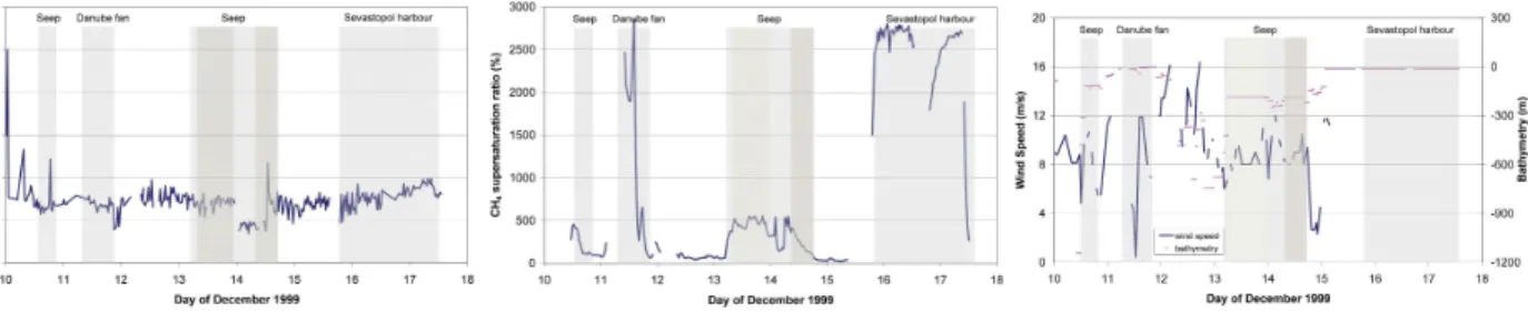
Fig. 1.Methane mixing ratios in air (left) and supersaturation ratios (middle) during the BIGBLACK cruise. Wind speed measurements and bathymetry time series are also plotted (right). Shaded areas denote ship’s location, while areas with darker shading indicate measurements where the vessel was anchored directly above active seeps. Areas denoted “Seep” are areas with active seeps.
Water temperature and salinity at 4 m (the depth where the water pump inlet was located) were measured with CTD
sondes during the cruise. The deviations (1σ ) of these
two parameters during the cruise were small (temperature: 10.68±0.29, salinity 17.6±0.34), hence their mean values were used in all calculations. Two pressure-equilibrating tubing lines in the equilibrator ensured sampling under at-mospheric pressure, hence no pressure correction had to be applied.
We also established that the equilibration time of the sea-water equilibrator (around 15 min) might have caused, in the case of rapidly fluctuating concentrations, a smoothing of the measured seawater concentrations while sampling en route. This does not affect the measurements performed at the sta-tions visited during the cruise (active seep areas and Sev-astopol harbour). Furthermore, the system performed with-out any problems for the duration of the cruise and we were able to calculate supersaturation ratios and fluxes of methane from the cruise area to the atmosphere.
Wind measurements were made with the ship anemome-ter, at 10.78 m height ASL, on a ship mast of 4.75 m height, hence eliminating the need for corrections of the wind speed
u to u10. These data were provided by the ship operator,
and consist of measurements of wind speed and direction provided twice an hour. No details on the averaging times were provided. The data were corrected for ship’s move-ment, based on concurrent data on ship’s velocity and head-ing. Clearly, no such correction was applied for the times the ship was anchored.
The model used for calculating the dispersion of the methane plume from mud volcano eruptions is the 3-D air-shed model ISC-AERMOD from Lakes Environmental Inc. (The et al., 2002), modified to accommodate a larger grid (original grid 50 km×50 km). The model calculated the con-centrations at 100×100 grid point receptors. It is a steady-state Gaussian plume dispersion model, based on U.S. Envi-ronmental Protection Agency’s ISCST3 model (EPA, 1995). It calculates ground-level and aloft inert ambient pollutant concentrations and deposition fluxes, for continuous and/or accidental releases (per hour). The model can handle
mul-tiple sources including point, volume, area, open pit as well as line source types. Source emission rates can be treated as constant or may be varied by month, season, hour-of-day, or other optional periods of variation. These variable emission rate factors may be specified for a single source or for a group of sources. In addition, the underlying ISCST3 model includes several options for addressing complicated problems like site-specific wind profile exponents, vertical potential temperature gradients, time-dependent exponential decay of emissions, plume rise calculated as a function of downwind distance, etc.
Required inputs are the wind velocity (see below for the wind velocity used for the three simulated atmospheric stability classes) and direction (various), relative humidity (60%), temperature (288 K), pressure (1024 mb) and atmo-spheric stability class (D-neutral, F-stable and A-unstable). The mixing height was set to 1000 m.
3 Results and discussion
The determined concentrations of methane in air and sea-water, the calculated super-saturation ratios, as well as wind speed measurements and bathymetry time series are pre-sented in Figs. 1 and 2. The ship left the harbour of Istan-bul on the 9 December 1999. Very high values of methane in air equilibrated with seawater lead to the saturation of the FID detector of the analytical system, hence inhibiting quan-titative determination of the very high methane seawater su-persaturations while in the harbour. Further, upon departure of the ship, the propeller caused sediment to enter the sys-tem; hence the measurements were resumed, after extensive cleaning, on the 10 December. On the 10 December, the ship sampled in open waters, over an active seep area, and over shelf waters. On the 11, the Danube fan area was sampled. On the 13 and the 14, a large part of the time was spent per-forming stations above active seep areas. The ship arrived outside the port of Sevastopol in the night of the 15 and re-mained anchored there before entering the port of Sevastopol early in the morning of the 16, where measurements contin-ued until the afternoon of the 17.
Fig. 2.Methane mixing ratios in water (in ppmv) during the BIG-BLACK cruise plotted as a function of date (above) and as a func-tion of posifunc-tion (below). The 1:250 000 resolufunc-tion coastline is from NOAA’s National Geophysical Data Centre. Shaded areas are as in Fig. 1. The arrows in the bottom figure denote the date (day of De-cember, 00:00 h). Bathymetry contours are also shown (bottom, in metres).
The wind velocity during the cruise varied mostly between
6 and 10 m s−1, while on occasions it fell below 6 m s−1or
rose above 10 m s−1(Fig. 1, right). The depth varied between
10 m and 1100 m (Fig. 1, right), while the mixed layer depth, as determined from CTD measurements during the cruise, was generally between 20 and 50 m.
Above the two active seep areas where the ship sam-pled on the 10 and almost the entire 13 and 14 December, methane concentrations in seawater were 8–20 ppmv, result-ing in super-saturation ratios 100–550%. In the Danube fan area, where the ship sampled on the 11 December, methane concentrations in seawater were up to 90 ppmv, resulting in super-saturation ratios of up to nearly 3000%, many times higher than in the active seep areas. These high concentra-tions are the result of the nutrient discharge from the Danube river, the nutrients coming from agricultural fertiliser appli-cations within the river basin and settlement effluent along the river course.
Fig. 3.Flux densities calculated after LM86, W92 and MG01 using the measured wind speed (lines). Dots are calculations after MG01 using the climatic wind speed value of 8 m/s. Shaded areas are as in Fig. 1.
In the port of Sevastopol, where the ship sampled from the end of the 15 until the 17 December, methane concentrations in seawater were up to 92 ppmv, resulting in super-saturation ratios of up to nearly 3000%, also many times higher than in the active seep areas. The high concentrations in the ports of Sevastopol and Istanbul are indicative of high nutrient and organic load in the sediments, probably because of urban sewage effluent. Measurements were also obtained during stations directly above active seeps (Figs. 1 and 2). The mea-surements during the stations were made on two occasions, the 13 December from 08:00 to 20:05 and the 14 December from 08:10 to 17:30, while the vessel was anchored at a depth
of around 180 m. While during the first station the CH4
con-centration in water did not vary much (15–21 ppmv), during the second one there were variations of a factor of two (7– 15 ppmv). While it appears that in the former case the plume of dissolved methane was more uniform, in the latter one this was not the case. Heterogeneity in the near-field dissolved methane plume has been observed earlier (Clark et al., 2000), although at distances larger than the ones in our case, and hence on the second station measurements might have been influenced either by changing currents or the ship’s drifting around the anchor, or both.
Flux densities (Fig. 3), as already mentioned, were cal-culated using the methodology described in detail in Bange (1994) and Bange et al. (1994), using the parameterisations of the dependency of the transfer velocity on wind speed of LM86, W92 and MG01 (see Introduction), and the mea-sured wind speed. Flux densities were also calculated using the latest parameterisation, MG01, and the climatic value of
wind speed for December, 8 m s−1(Sorokin, 2002; NEMOC,
2006). Lacking wind speed measurements during the ship’s stay in the port of Sevastopol, flux densities with actual wind speeds were not calculated, but they should probably be higher than above active seeps, as the flux calculations
K. Kourtidis et al.: Effects of methane outgassing on the Black Sea atmosphere 5177 Quite high flux densities were also calculated for the Danube
fan area. Generally, flux densities are higher than the ones obtained in our group’s cruise in the same area during July 1995 (Amouroux et al., 2002) and also higher than the val-ues reported by Schmale et al. (2005), obtained during May-June 2003. In open and shelf waters, Amouroux et al. (2002)
measured flux densities of 50–53 umol m−2day−1, Schmale
et al. (2005) measured 49 umol m−2day−1(calculated with
W92), while the measurements reported here range between
22–260 umol m−2day−1(calculated also with W92) for open
and shelf waters. A part of the difference might be explained by lower wind speeds during the Amouroux et al. (2002)
study, the climatic value for July being 5 m s−1as compared
with 8 m s−1for December (Sorokin, 2002; NEMOC, 2006),
and the exceptionally low wind speeds during the Schmale
et al. (2005) measurements (1.16 m s−1). Fluxes during the
present study above active seep areas during the 10, the 13
and the 14 December were up to 480 umol m−2day−1 and
measurements at the Danube fan on the 11 December were
up to 3150 umol m−2day−1(W92). At the high wind speeds
of the 11 and the 12 December (up to 16 m s−1), differences
are observed between the cubic (LM86) and the quadratic parameterisations (MG01 and W92), the latter increasing the calculated wind densities by approximately a factor of two (Fig. 3), while at low wind speeds substantial differences (up to a factor of two) result also between MG01 and W92, the former being higher. Flux calculations with MG01 were
per-formed also for the climatic value of wind speed, 8 m s−1
and are also presented in Fig. 3. Generally, since the mean wind during the campaign was near the climatic value, the differences in the flux calculations are not very big when the climatic wind speed value is used, except for the cases where the wind deviated significantly from the climatic value.
We used a simple method to estimate the effects of the
above fluxes on the atmospheric concentrations of CH4:
We assume a box located above the sea, with its ceiling at 1000 m, which appears a reasonable assumption for the height of the mixing atmospheric layer. The box is ventilated by the horizontal wind, for which we use the values that were measured during the BIGBLACK cruise onboard R/V “Pro-fessor Vodianitskiy” (as measured with the LM86
parameter-isation, climatic value of 8 m s−1with the MG01
parameter-isation). If we assume that methane is vented into the box with the flux densities of Fig. 3 (LM86 and MG01), and the contents of the box are vented completely out of the box in the time required for the mean wind speed to cross the box from one side to the other, with a series of simple calculations we derive that the measured flux densities would result in an increase in the atmospheric mixing ratio of methane by the amounts given in Fig. 4, which do not exceed a few tens parts per trillion per volume (pptv). Clearly, under normal condi-tions the air-sea exchange of methane from the Black Sea has a negligible impact on the regional atmospheric background of methane, being many times smaller than the observed vari-ability of atmospheric methane (Fig. 1a).
Fig. 4. Calculated increases (in parts per trillion per volume) in the atmospheric methane concentration due to the measured fluxes (using the LM86 parameterisation with measured wind speeds and the MG01 parameterisation with the climatic wind speed value). Shaded areas are as in Fig. 1. See also text.
3.1 Eruption scenarios
We note here that even the most intensive Black Sea bubble seep that was studied within the BIGBLACK and CRIMEA projects does not transfer methane into the atmosphere through bubble transport, which would be a more efficient means than dissolved methane for transferring methane to the atmosphere. Only at depths shallower than 90 m can some of the methane survive in the bubbles to reach the atmosphere, but this is probably very minor (McGinnis et al., 2006). At greater depths, all methane is dissolved from the bubbles long before they reach the surface. The same holds true for mud volcanoes at about 2080 m depth that were monitored during the CRIMEA project. During simultaneous eruptions from three mud volcanoes, the bubbles could be observed on the echo sounder rising 1300 m in the water column (Greinert et al., 2006; McGinnis et al., 2006). Therefore, in order for a significant methane input into the atmosphere to occur, a much more massive outgassing is needed. This seems rather unlikely for the shallower seep areas (100–600 m) given the diffuse nature of the seeping process. However, it does not seem impossible for a significant mud volcano eruption to generate a much larger methane bubble flux, with bigger bubbles and possibly even creating a bubble plume, which could eventually make it up to the atmosphere. We now examine the case of episodic outbursts due to mud volcano eruptions. We assume underwater eruptions, where a por-tion of the emitted methane rises all the way from the sea floor to the sea surface, passes the pycnocline and then is re-leased to the atmosphere. We assume the release to the atmo-sphere occurs from a square area source 100 m×100 m. Sev-eral authors report self-ignition of the expelled gas from mud volcanoes (Aliyev et al., 2002; Bagirov et al., 1996a, b; Je-vanshir, 2002; Kugler, 1939), even for underwater eruptions (Sokolov, 1969). However, whether self-ignition is common
(a) 0 5 10 15 20 25 30 35 40 0 10 20 30 40 50
Distance from Source (km)
C H4 Pe rtu rb a ti o n (PPM ) StabilityA StabilityD (b) 0 100 200 300 400 500 600 0 10 20 30 40 50
Distance from Source (km)
C H4 Pe rtu rb a ti o n (PPM ) StabilityF (c) 0 50,000 100,000 150,000 200,000 250,000 300,000 0 10 20 30 40 50
Distance from Source (km)
C H4 Pe rtu rb a ti o n (PPM ) StabilityA StabilityD (d) 0 200,000 400,000 600,000 800,000 1,000,000 1,200,000 0 10 20 30 40 50
Distance from Source (km)
C H4 Pe rtu rb a ti o n (PPM ) StabilityF
Fig. 5. Calculated increases in the atmospheric background of methane for two cases of unignited eruptions under different atmo-spheric conditions. (a) and (b): An underwater eruption of 22.5 million m3 methane at shallow depths, with 0.09% of the emit-ted methane reaching the surface, is assumed (see text). The wind speed used in the calculations was 3 m s−1, 8 m s−1and 12 m s−1, for stability classes A and D (a) and F (b), respectively. (c) and (d): An underwater eruption of 323 million m3methane at 2 km depth, with 30% of the emitted methane reaching the surface, half of it in gaseous form within the bubbles, is assumed (see text). The wind speed used in the calculations was 3 m s−1, 8 m s−1and 12 m s−1, for stability classes A and D (c) and F (d), respectively.
in underwater eruptions and under which circumstances it might occur in nature, are, to our knowledge, not well docu-mented, hence no simulations for ignited emission were per-formed. Two eruption scenarios are examined. In both cases, we assume the eruptions last for 4 h, and underwater emis-sion rates are taken from Guliev (1992). Guliev (1992), p. 7, quoted extensively in the western peer-reviewed literature (e.g. in Kopf, 2002) and Guliyiev and Feizullayev (1994), also quoted extensively (e.g. in Dimitrov, 2002), state that for four prominent mud volcano eruptions in Azerbaijan be-tween 1902–1961 (on land), the amount of gas expelled
dur-ing the first few hours ranged from 22.5–495 million m3. We
note here that Guliev (1992) has performed the only exten-sive study on quantitative eruptive methane emissions from mud volcanoes; apart from this study, only sporadic data are published. However, these infrequent data (summarized in Dimitrov, 2002) yield estimates of methane expelled during
the eruptive phase that range from 210 million m3to 40
bil-lion m3CH4over 1–2 days. Hence for the simulations
pre-sented here two cases were modelled, one eruption near the lower end of Guliev’s (1992) estimates, and one near the up-per end.
The first case presents a set of simulations for different atmospheric conditions for a small underwater eruption of
22.5 million m3methane, occurring at shallow depths, where
an estimated 0.09% of the methane reaches the atmosphere. The second case presents a set of simulations for different at-mospheric conditions for a large underwater eruption of 323
million m3methane, occurring at a depth of 2 km, where an
estimated 30% of the methane reaches the atmosphere. More details on the simulations and the assumptions involved are given below. For both cases, the fraction of methane that reaches the air-sea interface was estimated using the bub-ble model of McGinnis et al. (2006) in combination with the modified (for deep water conditions) bubble plume model of W¨uest et al. (1992).
In the first case, a small underwater eruption of 22.5
mil-lion m3methane (at the lower end of Guliev, 1992) is
simu-lated. Following results from recent work on bubble-water column exchange of gases in the frame of the CRIMEA project (McGinnis et al., 2006), it appears that for such small emission rates, the eruption has to occur at relatively shal-low depths, for even a small fraction of the methane to reach the surface. These results show that in the worst case 0.09% of the methane gas might reach the atmosphere. We assume the release to the atmosphere occurs from a rectangular area source 100 m×100 m, hence the emission rate in this case is
6.25 mmol m−2s−1(or 1000 g s−1).
These modelling results (Figs. 5a, b) suggest that even rel-atively small methane outbursts from mud volcanism may result in very large enhancements in the regional methane concentrations near the sea surface. For unstable and neu-tral conditions, the release results in raising the atmospheric methane concentration by 1–40 ppmv in the first 5 km down-wind from the release site, falling off at greater distances.
K. Kourtidis et al.: Effects of methane outgassing on the Black Sea atmosphere 5179 Under nighttime stable conditions (Fig. 5b), the
enhance-ment can reach 600 ppmv close to the source, creating smog chamber conditions. The larger computed increases propa-gate also at larger distances (for 30 km downwind methane is increased by more than 7 ppmv, falling to its atmospheric mixing ratio of 1.8 ppmv after 50 km). Given that the dis-persion model is linear (i.e. a doubling of the emission rate will double the concentrations), if a larger proportion of the methane reaches the atmosphere, concentrations will be pro-portionally larger.
In the second case, a massive underwater eruption of 323
million m3 methane (near the upper end of Guliev, 1992),
occurring at a depth of 2 km, is simulated. This translates to
16 000 000 g s−1. The amounts of methane that might rise to
the sea/atmosphere interface from such a massive methane release at 2 km depth have been estimated in the frame of the CRIMEA project. The initial conditions of the bubble model assume an initial plume radius of 100 m and a bubble diam-eter of 8 mm. The model has been run for various emission
rates; it appears that 16 000 000 g s−1is near the minimum
emission rate required for copious amounts of the methane
to reach the surface from 2 km depth. At this emission
rate, roughly 30% of the methane reaches the atmosphere in both gaseous and dissolved form (about 50% in bubbles and
50% dissolved), while at emission rates of 1 600 000 g s−1
no methane reaches the surface. On the other hand,
simulat-ing a mud volcano gas release of 24 500 000 g s−1 (i.e. 495
million m3, the upper end of emission rates given by Guliev,
1992) at 2 km depth, all of the methane reaches the surface (about 20% in bubbles and 80% dissolved). These simula-tions assume that a hydrate skin exists on the bubble in the stability zone (see, e.g., McGinnis et al., 2006; Rehder et al., 2002; Sauter et al., 2006). If no hydrate skin exists on the bubble, then the plume does not reach the surface. As mentioned above, bubble modelling estimates that 30% of the emitted gas reaches the atmosphere, about 50% of the methane residing in the bubbles and about 50% dissolved. The plume water when it reaches the surface is denser, so it is difficult to estimate with certainty how much the dis-solved fraction will degass before settling back to the equi-librium depth. Hence for the atmospheric dispersion mod-elling we assume that the direct bubble transfer is more effi-cient than the diffusion of dissolved methane, and neglect the latter in the calculation of emission rates to the atmosphere, arriving at an equivalent emission rate to the atmosphere of
15 mol m−2s−1, or 2400 kg s−1. Assuming the release takes
place from an area source 100 m×100 m, the maximum in-creases in the atmospheric levels of methane during the 4-h constant rate eruption as estimated through dispersion mod-elling with ISC-AERMOD, are given in Figs. 5c, d.
The plume dispersion modelling results for the second
case (i.e. a 323 million m3methane eruption at 2 km depth)
show that the spatial average of the methane perturba-tion (i.e. the increase above the background levels) dur-ing the eruption over a square receptor area with
dimen-sion 100 km×100 km centred in the source (assuming a 4-hour release) is approximately 4 ppmv for unstable condi-tions (A), 10 ppmv for neutral condicondi-tions (D) and 20 ppmv for stable conditions (F), which represent increases of the average background methane mixing ratio of 1.86 ppmv over the Black Sea of 315%, 640% and 1175%, respectively.
3.2 Considerations for remote sensing detection
Assuming that the concentrations of methane above the mix-ing height remain unaffected at 1.86 ppmv, a tropopause height of 10 km and negligible methane concentrations above the tropopause, these correspond to columnar increases of atmospheric methane of 146%, 216%, and 331% for these three stability classes, respectively.
Similarly, the spatial 24-h average of the methane per-turbation over a square receptor area with dimension 100 km×100 km centred in the source (also assuming a 4-h release) is approximately 0.7 ppm for unstable conditions (A), 2.7 ppm for neutral conditions (D) and 6.5 ppm for sta-ble conditions (F). The wind velocity field was 3, 8 and 12 (m/s) for the stability classes A, D and F, respectively (the perturbation amount will be generally higher for lighter winds). Hence, given an average background methane mix-ing ratio of 1.86 ppmv over the Black Sea, the calculated in-crease of the 24-h average mixing ratio of methane over the 100 km×100 km area ranges from 35% for unstable condi-tions to 350% for stable condicondi-tions. Again, these correspond to 24-h average columnar increases of atmospheric methane of 108%, 131%, and 175% for the three simulated stability classes A, D and F, respectively.
Clearly, these perturbations of the columnar amounts over the eruption time (4 h) and over the next 24 h following the eruption are fairly larger than the few percent perturbations required for the detection of emissions by space-borne in-strumentation such as the SCIAMACHY instrument onboard ENVISAT.
Given the steady improvement of algorithms for the detec-tion of methane from space (e.g. Buchwitz et al., 2000, 2005; Meirink et al., 2006) we would argue here that the detec-tion of either fairly large underwater mud volcano erupdetec-tions or modest ones over land might be possible with available space-borne instrumentation, providing perhaps a means for remote sensing of mud volcano eruptions. Generally, the typ-ical spatial resolution of the SCIAMACHY instrument on-board ENVISAT is 30 km by 60 km. Each horizontal scan of the atmosphere in limb covers 960 km in the horizontal (across track direction), and global coverage is achieved after 6 days (Bovensmann et al., 1999). SCIAMACHY consists of eight main spectral channels and seven spectrally broad band Polarization Measurement Devices (PMDs) (details are given in Bovensmann et al., 1999). Observations of channel 8 (from a small spectral fitting window 2265–2280 nm) and PMD number 1 (320–380 nm) have been used in the
detec-tion of CH4(Buchwitz et al., 2000, 2005). Channel 8 spectral
resolution is 0.2 nm. For SCIAMACHY the spatial resolu-tion, i.e., the footprint size of a single nadir measurement, de-pends on the spectral interval and orbital position. For chan-nel 8 the spatial resolution is 30 km×120 km corresponding to an integration time of 0.5 s, except at high solar zenith an-gles, where the pixel size is twice as large (30 km×240 km). Using various bias corrections improved methane data prod-ucts have been generated (e.g. Buchwitz et al., 2005); their comparison with model simulations shows agreement within a few percent (mostly within 5%).
The main scientific application of the methane measure-ments of SCIAMACHY is to obtain information on the sur-face sources of methane (e.g. Frankenberg et al., 2005). The modulation of methane columns due to methane sources (other than mud volcano eruptions) is only on the order of a few percent and typically, the weak methane source signal is difficult to be clearly detected with single overpass SCIA-MACHY data, unless the variations in atmospheric methane exceed a few percent. Applications of existing algorithms have shown that SCIAMACHY can detect elevated methane columns resulting from emissions from surface sources such as rice fields and wetlands over India, southeast Asia and cen-tral Africa (Buchwitz et al., 2005; Frankenberg et al., 2005). Hence, considering also the modelling results of the present study, it appears that certain events of mud volcano eruptions are very well above the sensitivity of satellite in-struments such as SCIAMACHY. It also appears that eleva-tions in the columnar methane amounts following some of the eruptions would persist long enough over areas compara-ble with the satellite footprint. This means, given that global coverage is achieved with ENVISAT every 6 days, and that the elevations survive for about 24 h at detectable levels, that a fair fraction (perhaps 10–20%) of the elevations in atmo-spheric concentrations caused by such massive events in a given region might survive until the next ENVISAT overpass. Although the present study neither offers a complete assess-ment for the extent of the applicability of satellite monitoring of mud volcano eruptions, nor fully constrains this, it offers nevertheless results that show that such an assessment study might prove very useful.
Further, very little is known about the size-frequency dis-tribution of such eruptive events. Apart from Guliev (1992), Jakubov (1971) provides statistics for 32 eruptions in Eastern Azerbaijan considering that 122 eruptions have occurred dur-ing the period 1840–1967. Ali-Zade et al. (1984) state that 200 eruptions in 50 mud volcanoes have occurred in East-ern Azerbaijan from 1910 to 1980, while Ridd (1970) shows a time interval of 1–22 years for mud volcanoes in New Zealand. Dimitrov (2002) summarises these and other data to infer, “with great skepticism”, as the author states, that about 30 mud volcanoes of Lokbatan type and 10 ones of the Schugin type erupt every year. Since it appears that at least certain events might be observable from space, a more thor-ough assessment of the possible range of events that might fall within the sensitivity limits of space-borne sensors and
the possible fraction of the time that these events might occur within the observing satellite swath without obscuring inter-ferences (e.g. clouds) might ultimately prove very useful not only in observing these events, but also in obtaining an idea, from space-borne observations, about the frequency-size dis-tribution of such events.
Acknowledgements. The authors wish to thank the captain and
crew of R/V “Professor Vodyanitskiy”. Also, we would like to acknowledge the exchange of ideas with the partners of the BIGBLACK and CRIMEA projects. This work was funded under the BIGBLACK (EU IC15 CT96 0107) and CRIMEA (EVK-2-CT-2002-00162) European Commission projects. Edited by: W. E. Asher
References
Aliyev, A., Guliev, I. S., and Belov, I. S: Catalogue of recorded eruptions of mud volcanoes of Azerbaijan, Nafta Press, Baku, 2002.
Ali-Zade, A., Shnyokov, E., Grigorianz, B., Aliev, A., and Rah-manov, R.: Geotectonic conditions of mud volcano manifestation on the Earth and their significance for oil and gas prospects (in Russian), Proc. 27th World Geol. Congr. C13, 166–172, 1984. Amouroux, D., Roberts, G., Rapsomanikis, S., and Andreae, M.
O.: Biogenic Gas (CH4, N2O) Emission to the Atmosphere from Near-shore and Shelf Waters of the North Western Black Sea, Estuarine, Coastal Shelf Sci., 54(3), 575–587, 2002.
Bagirov, E., Nadirov, R., and Lerche, I.: Flaming eruptions and ejections from mud volcanoes in Azerbaijan: Statistical risk as-sessment from the historical records, Energy Explor. Exploit., 14, 535–583, 1996a.
Bagirov, E., Nadirov, R., and Lerche, I.: Earthquakes, mud volcano eruptions, and fracture formation hazards in the South Caspian basin: Statistical inferences from the historical record, Energy Explor. Exploit., 14, 585–606, 1996b.
Bange, H. W., Bartell, U. H., Rapsomanikis, S., and Andreae, M. O.: Methane in the Baltic and North Seas and a reassessment of marine emissions of methane, Global Biogeochem. Cycles, 8, 465–480, 1994.
Bange, H. W.: Messungen von Lachgas (N2O) und Methan (CH4)in Europaeischen Nebenmeeren, Ph.D. Thesis, Johannes Gutenberg-Universitaet, Mainz, 1994.
Bange, H. W., Rapsomanikis, S., and Andreae, M. O.: The Aegean Sea as source of atmospheric nitrous oxide and methane, Marine Chem., 53, 41–49, 1996.
Bovensmann, H., Burrows, J. P., Buchwitz, M., Frerick, J., No¨el, S., Rozanov, V. V., Chance, K. V., and Goede, A. P. H.: SCIAMACHY- Mission Objectives and Measurement Modes, J. Atmos. Sci., 56, 127–149, 1999.
Buchwitz, M., Rozanov, V. V., and Burrows, J. P.: A near infrared optimized DOAS method for the fast global retrieval of atmo-spheric CH4, CO, CO2, H2O, and N2O total column amounts from SCIAMACHY/ENVISAT-1 nadir radiances, J. Geophys. Res., 105, 15 231–15 246, 2000.
Buchwitz, M., de Beek, R., Noel, S., Burrows, J. P., Bovensmann, H., Bremer, H., Bergamaschi, P., Koerner, S., and Heimann,
K. Kourtidis et al.: Effects of methane outgassing on the Black Sea atmosphere 5181
M.: Carbon monoxide, methane and carbon dioxide columns re-trieved from SCIAMACHY by WFM-DOAS: year 2003 initial data set, Atmos. Chem. Phys., 5, 3313–3329, 2005,
http://www.atmos-chem-phys.net/5/3313/2005/.
Butler, J. H., Elkins, J. W., Brunson, C. M., Egan, K. B., Thompson, T. M., Conway, T. J., and Hall, B. D.: Trace gases in and over the West Pacific and East Indian Oceans during the El Nino-Southern Oscillation event of 1987, NOAA Data Report ERL ARL-16, Air Resources laboratory, Silver Spring, MD, USA, 1988.
Butler, J. H., Elkins, J. W., Thompson, T. M., and Egan, K. B.: Tropospheric and dissolved N2O off the West Pacific and Indian Oceans during the El Nino-Southern Oscillation event of 1987, J. Geophys. Res., 94, 14 865–14 877, 1989.
Clark, J. F., Washburn, L., Hornafius, J. S., and Luyendyk, B. P.: Dissolved hydrocarbon flux from natural marine seeps to the southern California Bight, J. Geophys. Res., 105, 11 509–11 522, 2000.
Cynar, F. J. and Yayanos, A. A.: Distribution of methane in the upper waters of Southern California Bight, J. Geophys. Res., 97, 11 269–11 285, 1992.
Dimitrov, L. I.: Mud volcanoes – the most important pathway for degassing deeply buried sediments, Earth-Sci. Rev., 59, 49–76, 2002.
Durisch-Kaiser, E., Klauser, L., Wehrli, B., and Schubert, C.: Ev-idence of intense archaeal and bacterial methanotrophic activity in the Black Sea water column, Appl. Environ. Microbiol., 71, 8099–8106, 2005.
EPA: User’s Guide for the Industrial Source Complex (ISC3) Dis-persion Models/ Volume I – User Instructions, US EPA, Office of Air Quality Planning and Standards, Emissions Monitoring and Analysis Division, Research Triangle Park, NC 27711. Report number EPA-454/B-95-003a, 1995.
Etiope, G. and Klusman, R. W.: Geologic emissions of methane to the atmosphere, Chemosphere, 49, 777–789, 2002.
Fairall, C. W., Hare, J. E., Edson, J. B., and McGillis, W.: Parame-terisation and micrometeorological measurements of air-sea gas transfer, Boundary-Layer Meteorol., 96, 63–105, 2000. Feely, R. A., Wanninkhof, R., McGillis, W., Karr, M.-E., and Cosca,
C. E.: Effects of wind speed and gas exchange parameterisations on the air-sea CO2fluxes in the equatorial Pacific Ocean, J. Geo-phys. Res., 109, C08S03, doi:10.1029/2003JC001896, 2004. Frankenberg, C., Meirink, J. F., van Weele, M., Platt, U., and
Wag-ner, T.: Assessing methane emissions from global spaceborne observations, Science, 308, 1010–1014, 2005.
Greinert, J., Artemov, Y., Egorov, Y., De Batist, M., and McGinnis, D.: 1300-m high rising bubbles from mud volcanoes at 2080 m in the Black Sea: Hydroacoustic characteristics and temporal vari-ability, Earth Planet. Sci. Lett., 244, 1–15, 2006.
Guliev, I. S.: A review of mud volcanism, Report, 65 pp., Inst. of Geol., Azerbaijan Acad. of Sci., Baku, 1992.
Guliyiev, I. S. and Feizullayev, A. A.: Natural hydrocarbon seep-ages in Azerbaijan, Proc. AAPG Hedberg Research Conference, 24–28 April, Vancouver, Canada, 76–79, 1994.
Hare, J. E., Fairall, C. W., McGillis, W. R., Edson, J. B., Ward, B., and Wanninkhof, R.: Evaluation of the NOAA/Coupled-Ocean Atmopheric Response Experiment (NOAA/COARE) air-gas tranfer parameterization using GasEx data, J. Geophys. Res., 109, C08S11, doi:10.1029/2003JC001831, 2004.
Hornafius, J. S., Quigley, D., and Luyendyk, B. P.: The world’s most
spectacular marine hydrocarbon seeps (Coal Oil Point, Santa Barbara Channel, California): quantification of emissions, J. Geophys. Res., 104, 20 703–20 711, 1999.
IPCC, Climate Change 2001: Third Assessment – The Scientific Basis, IPCC, Geneva, Switzerland, 2001.
Jakubov, A. A., Ali-Zade, A. A., and Zeinalov, M. M.: Mud volca-noes of the Azerbaijan SSR: Atlas, Elm-Azerbaijan Acad. of Sci. Baku, 1971.
Jevanshir, R. D.: All about mud volcanoes, 97 pp., Inst. Of Geol., Azerbaijan Acad. of Sci., Baku, 2002.
Judd, A. G., Davies, G., Wilson, J., Holmes, R., Baron, G., and Bry-den, I.: Contributions to atmospheric methane by natural seep-ages on the UK continental shelf, Marine Geol., 137, 427–455, 1997.
Klusman, R. W., Leopold, M. E., and LeRoy, M. P.: Seasonal vari-ation in methane fluxes from sedimentary basins to the atmo-sphere: Results from chamber measurements and modelling of transport from deep sources, J. Geophys. Res., 105D, 24 661– 24 670, 2000.
Kopf, A. J.: Significance of mud volcanism, Rev. Geophys., 40, 1005, doi:20.1029/2000RG000093, 2002.
Kugler, H. G.: Visit to Russian oil districts, J. Inst. Pet. Technol. Trinidad, 25(184), 68–88, 1939.
Kvenvolden, K. A.: Gas hydrates-Geological perspective and global change, Rev. Geophys., 31, 173–187, 1993.
Lelieveld, J., Crutzen, P. J., and Br¨uhl, C.: Climate effects of atmo-spheric methane, Chemosphere, 26, 739–768, 1993.
Lelieveld, J., Crutzen, P., and Dentener, F. J.: Changing concentra-tion, lifetime and climate forcing of atmospheric methane, Tel-lus, 50B, 128–150, 1998.
Liss, P. S. and Merlivat, L.: Air–sea exchange rates: introduction and synthesis, in The role of air-sea exchange in geochemical cycling, edited by: Buat-Menard, P., 113–127, Reidel, D., New York, 1986.
McGillis, W. R., Edson, J. B., Ware, J. D., Dacey, J. W. H., Hare, J. E., Fairall, C. W., and Wanninkhof, R.: Carbon dioxide flux techniques performed during GasEx-98, Mar. Chem., 75, 267– 280, 2001.
McGillis, W. R., Asher, W.E., Wanninkhof, R., Jessup, A.T., and Feely, R.A.: Introduction to special section: Air-sea exchange, J. Geophys. Res., 109, C08S01, doi:10.1029/2004JC002605, 2004. McGinnis, D. F., Greinert, J., Artemov, Y., Beaubien, S. E., and W¨uest, A.: Fate of rising methane bubbles in stratified waters: How much methane reaches the atmosphere?, J. Geophys. Res., 111, C09007, doi:10.1029/2005JC003183, 2006.
Meirink, J. F., Eskes, H. J., and Goede, A. P. H.: Sensitivity analysis of methane emissions derived from SCIAMACHY observations through inverse modelling, Atmos. Chem. Phys., 6, 1275–1292, 2006,
http://www.atmos-chem-phys.net/6/1275/2006/.
NEMOC: Naval European Meteorology and Oceanography Com-mand, available online at https://www.nemoc.navy.mil/index. html, 2006.
Olsen, A., Wanninkhof, R., Trinanes, J. A., and Johannessen, T.: The effect of wind speed products and wind speed-gas exchange relationships on interannual variability of the air-sea CO2gas transfer velocity, Tellus, 57B, 95–106, 2005.
Rehder, G., Brewer, P. W., Peltzer, E. T., and Friedrich, G.: Enhanced lifetime of methane bubble streams within
the deep ocean, Geophys. Res. Lett., 29(15), 1731, doi:10.1029/2001GL013966, 2002.
Ridd, M. F.: Mud volcanoes in New Zealand, AAPG Bull., 54, 601– 616, 1970.
Sauter, E. J., Muyakshin, S. I., Charlou, J.-L., Schlueter, M., Boetius, A., Jerosch, K., Damm, E., Foucher, J.-P., and Klages, M.: Methane discharge from a deep-sea submarine mud volcano into the upper water column by gas hydrate-coated methane bub-bles, Earth Planet. Sci. Lett., 243, 354–365, 2006.
Schmale, O., Greinert, J., and Rehder, G.: Methane emis-sion from high-intensity marine gas seeps in the Black Sea into the atmosphere, Geophys. Res. Lett., 32, L07609, doi:10.1029/2004GL021138, 2005.
Sokolov, V., Buniat-Zade, Z., Geodekian, A., and Dadashev, F.: The origins of gases of mud volcanoes and the regularities of power-ful eruptions, Advances in Organic Chemistry, Pergamon, Ox-ford, 473–484, 1969.
Sorokin, Y. I.: The Black Sea Ecology and Oceanography. Back-huys Publishers, Leiden, The Netherlands, 2002.
The, J. L., The, C., and Johnson, M.: ISC-AERMOD View User’s Guide, Lakes Environmental Software, Lakes Environmental Inc., 2002.
Wanninkhof, R.: Relationship between wind speed and gas ex-change over the ocean, J. Geophys. Res., 97(C5), 7373–7382, 1992.
Wanninkhof, R. and McGillis, W. R.: A cubic relationship between air-sea CO2exchange and wind speed, Geophys. Res. Lett., 26, 1889–1892, 1999.
Wanninkhof, R., Sullivan, K. F., and Top, Z.: Air-sea gas tran-fer in the Southern Ocean, J. Geophys. Res., 109, C08S19, doi:10.1029/2003JC001767, 2004.
Ward, B. B.: The subsurface methane maximum in the California Bight, Cont. Shelf Res., 12, 735–752, 1992.
Watson, A. J., Upstill-Goddard, R. C., and Liss, P. S.: Air-sea gas exchange in rough and stormy seas measured by a dual-tracer technique, Nature, 349, 45–147, 1991.
Weiss, R. F.: Determinations of carbon dioxide and methane by dual catalyst flame ionisation chromatography and nitrous oxide by electron capture chromatography, J. Chromatogr, Sci., 19, 611– 616, 1981.
Woolf, D. K.: Parametrization of gas transfer velocities and sea-state-dependent wave breaking, Tellus, 57B, 87–94, 2005. W¨uest, A., Brooks, N., and Imboden, N.: Bubble Plume Modeling
for Lake Restoration, Water Resour. Res., 28(12), 3235–3250., 1992.