Analysis and implementation of laboratory automation system

(1)

Analysis and Implementation of Laboratory Automation System

by

Rafael Garcia Secundo

B.S. Aerospace Engineering, North Carolina State University, 2006

Sloan School of Management and the Department of Mechanical Engineering in Partial Fulfillment of the Requirements for the Degrees of

MASTER OF BUSINESS ADMINISTRATION AND

MASTER OF SCIENCE IN MECHANICAL ENGINEERING

In conjunction with the Leaders for Global Operations Program at the Massachusetts Institute of Technology

June 2015 J z CD W7- -I Co ) Of M, L)u <4:

The author hereby grants to MIT permission to reproduce and to distribute publicly paper and electronic copies of this thesis document in whole or in part in any medium now known or hereafter created.

Signature of Author

Certified by

Accepted by

_______Signature

redacted

Department of Mechanical Engineerinr, MIT Sloan School of Management

May 8, 2015

______________Signature

redacted

Daniel Whitn Thesis Supe visor Senior Research Scientist, Emeritus, Engineering Sy s ivision

Signature redacted

-Z

Itai Ashlagi, Thesis Supervisor Associate Professor of Operations Management, MIkST an School of Ma agement

Sig-nature redacted

David Hardt, Chairman of the Committee on Graduate Students Department of Mechanical Engineering

Accepted by

Signature redacted

Maura -irson, Director of MIT Sloan MBA -1'ogram MIT Sloan School of Management Submitted to the MIT

(2)

This page intentionally left blank.

(3)

Analysis and Implementation of Laboratory Automation System

by

Rafael Garcia Secundo

Submitted to the MIT Sloan School of Management and the Department of Mechanical Engineering on May 8, 2015 in Partial Fulfillment of the Requirements for the Degrees of

Master of Business Administration and

Master of Science in Mechanical Engineering

Abstract

Quest Diagnostics is a large company that analyzes millions of medical specimens every day using a variety of analytical equipment. It is implementing a fully automated line in a major laboratory. The automation line is Quest's first major automation initiative and will serve as a pilot for future initiatives. An important element of implementing this initiative is the transition from manual to automated specimen handling operations. Furthermore, it is crucial to model the behavior of the newly automated production system. This thesis discusses the risk analysis performed on the transition from manual operations into automated as well as a discrete event simulation developed to model the automated system in its planned final state.

The risk analysis was performed by identifying the risks of the transition of each affected analyzer and scoring each risk based on its severity and probability of occurrence. A reduction factor was added for analyzers that were to be transitioned later in the sequence schedule to account for the ability of the team to learn with each equipment transition.

The simulation was based on existing process flow diagrams and populated with data from the two largest labs to be consolidated in Marlborough, MA, which comprise 90% of the expected volume. The

simulation results were then compared to a previously performed static simulation and to current data from the Marlborough lab, which is now operational. This revealed a discrepancy between the simulation and the current data in terms of total specimens processed at each analyzer. This is attributed to the differences between the current manual process and the expected automated process.

The dynamic model shows that the planned automation line can support the expected specimen volume even with 10% reduction in equipment efficiency. A planned 20% increase in volume was also evaluated along with its associated increase in capacity. The automation line can support the higher volume with the planned increase in capacity. Although these results are promising, further work is needed to validate the model results once the automation system is fully operational.

Thesis Supervisor: Daniel E. Whitney

Title: Senior Lecturer, Emeritus, Engineering Systems Division Thesis Supervisor: Itai Ashlagi

(4)

(5)

Acknowledgements

I would like to humbly thank everyone who have contributed to my work in this two-year journey that has been the Leaders for Global Operations program. Be it directly or indirectly by your support, I would not have survived the past two years and definitely would not have complete my thesis without you.

From Quest Diagnostics, who sponsored the project that spawned this thesis, I am grateful for the support of Denis Gallagher, Michael Hellyar, Chris Radke, and Fred Solomon. I would also like to thank Jesse Flippo, Margherita Walkowski, Chris Slavin, Mimi Perdue-Loan, and Susan Willeford for their continuous technical support. The results documented in this thesis would not have been possible without you.

From MIT, I would also like to thank my thesis advisors, Dr. Daniel Whitney and Dr. Itai Ashlagi for their invaluable advice and support of this project. Additionally, I would like to acknowledge the Leaders for Global Operations Program for its support of this work. Further thanks are given to all of my LGO colleagues who have made this journey a fantastic experience. And lastly, but most importantly, I would like to thank my wife, Megan, for her never waning

support over this crazy adventure that has been the past two years. I am absolutely certain that I would not be here if it were not for you.

(6)

(7)

List of Figures

Figure 1: Sample Automated System Layout...21

Figure 2: Specimen A Process Flow Chart... 30

Figure 3: Specimen B Process Flow... 30

Figure 4: Simulation M odel Architecture... 31

Figure 5: Master Simulation M odel... 32

Figure 6: Phase 1 Design - Baseline Results ... 42

Figure 7: Phase 1 Design - Baseline Utilization ... 43

Figure 8: Phase 1 Design - Average Cycle Times ... 44

Figure 9: Phase 1 Design - Total Queue Size ... 44

Figure 10: Phase 1 Design - 20% Increase in Volume ... 45

Figure 11: Phase 2 Design - Baseline Results ... 46

Figure 12: Phase 2 Design - Baseline Utilization ... 46

Figure 13: Phase 2 Design - Average Cycle Times ... 47

(11)

List of Tables

Table 1: Equipm ent Throughput Sum m ary... 34

Table 2: Data Sources...35

Table 3: Original M odel Daily Load Comparison... 37

Table 4: Adjusted M odel Daily Load Comparison ... 39

Table 5: Phase 2 Capacity Increase ... 40

Table 6: Risk Scores Sum m ary ... 53

(12)

(13)

1 Introduction

Quest Diagnostics (Quest) is the world's leading clinical laboratory operator, offering a broad range of diagnostic testing and interpretive consultation services to doctors and patients world-wide [1]. As the Affordable Healthcare Act comes into effect, there is greater pressure on

laboratories and providers to lower reimbursement from both private and federal payers [2]. This pressure drives independent laboratories to search for new ways to develop new efficiencies and

drive costs down.

In the effort to drive costs down and increase internal efficiency, Quest is consolidating various laboratories into a single facility in Marlborough, MA. This initiative will help Quest improve its operations and achieve economies of scale at the new regional laboratory. Integral to the design of the new laboratory in Marlborough is a comprehensive automation initiative. The new automation system will allow Quest to enhance quality and efficiencies while maintaining a relatively low cost to its diagnostic services [3].

1.1 Purpose of Project

The new automation line being implemented in Marlborough, MA is Quest's first major laboratory automation initiative and will serve as a pilot program for future initiatives. An important element of implementing this initiative is the transition from manual operations to automated operations. In order to successfully execute this transition with minimal impact to daily operations, it is paramount to analyze the risks associated with this undertaking and to mitigate them where appropriate.

After transition has been achieved, it is crucial to be able to model the throughput and behavior of the newly automated production system. Although a static capacity analysis has been

(14)

completed to guide the design of the automated line, a dynamic analysis will serve as a tool to guide future capacity and staffing decisions. At its core, the purpose of the project described in this thesis was to assist Quest in developing the base tools to quickly materialize their own internal goals with the automation initiative. More specifically, this project had very specific goals that are outlined in the next section and discussed in depth throughout this document.

1.2 Project Goals

The primary goals of the project, in support of its core purpose described previously, are outlined below.

" To perform a quantitative risk assessment of Quest's plan to transition from to automated specimen handling operations.

" To develop a risk mitigation plan and re-evaluate the risk assessment with the mitigation steps in place.

* To develop a discrete event simulation of the automated system and evaluate its performance under a variety of scenarios.

1.3 Project Approach

The research project that supports this thesis was performed at a Quest Diagnostics laboratory in Marlborough, MA. The approach taken throughout the project was to divide the three goals described above in two parallel tracks, one pertaining to the risk assessment and mitigation and the other to the discrete event simulation. The risk assessment track was divided in the following tasks.

1. Understand the transition plan that was already established by the company stakeholders. 2. Brainstorm to identify the risks associated with the transition.

(15)

3. Score each risk based on its severity and probability of occurrence.

4. Calculate the overall risk for each equipment platform being transitioned, while taking lessons learned opportunity into account.

5. Prioritize risks and equipment platforms based on total risk scores 6. Brainstorm mitigation measures.

7. Re-score each risk in light of the mitigation measures in place.

8. Update the overall risk based on the new scores.

The discrete event simulation was approached in the following tasks.

1. Understand the process flow for each specimen type processed by the automated system.

2. Build the sub-model for each specimen type.

3. Validate and troubleshoot the operation of each sub-model.

4. Integrate all sub-models into the master model.

5. Input simulation parameters based on data from existing manual operation system. 6. Run baseline simulation and compare results with existing performance data and

previously performed static capacity analysis.

7. Adjust simulation parameters to match existing data.

8. Perform a sensitivity analysis of the automation system by varying various system input

(16)

1.4 Thesis Overview

The thesis is structured as follows. Chapter 2 explores the background of Quest Diagnostics and its operations. It further describes the processes being automated and the underlying reasoning for the automation effort at Quest. Chapter 3 discusses some relevant work that has been performed in flexible manufacturing systems, risk analysis, and implementation of automated systems. Chapter 4 will describe in detail the methodology developed for the discrete event simulation supporting this thesis. Chapter 5 will discuss the results of the discrete event simulation analysis followed by its key findings. Chapter 6 will discuss the methodology and results of the risk analysis performed on the transition from manual to automated operations. Finally, Chapter 7 will provide the final conclusions of the analyses performed and provide recommendations for the automation system and future automation implementations at Quest as well as recommendations for further developments.

(17)

2 Automation at Quest

2.1 Background of Company

Quest Diagnostics was founded in 1967 as Metropolitan Pathology Laboratory, Inc., becoming an independent corporation in 1997 with the Quest name [4]. Since 1997, Quest has grown tremendously in its size and patient reach by investing in internal excellence and by acquiring complementary laboratories. Today, Quest employs approximately 45,000 people and touches the lives of approximately 30% of all adults in the US [1]. Furthermore, Quest operates laboratories in India, Europe, and Latin America.

2.2 Quest Laboratory Operations

Quest offers a broad range of diagnostics and testing services to its customers, ranging from the more simple blood chemistry tests to the more exoteric DNA sequencing tests. However, the description below only pertains to operations performed on blood and urine specimens that are performed by the automated system.

2.2.1 Specimens

The specimens are collected from patients by nurses and phlebotomists (blood collection specialists) at medical providers' offices, hospitals, and at Quest's collection sites. During the collection process, the test specimen (blood or urine) is stored in a collection tube that is

appropriate for the type of testing that will be performed. The specimen collection tubes contain chemicals or chemical treatments that are intended to preserve and prepare the specimen for the required tests. They may be made from glass or plastic and typically have color coded tops. Furthermore, the tops may be rubber stoppers or screw-caps. The automation system is designed to handle only plastic collection tubes for safety reasons. Also, it is only designed to handle screw-cap tops.

(18)

2.2.2 Test Requisitions

Quest serves a wide variety of medical providers and process test specimens that are collected by the providers' office, hospitals, and their own collection offices. Due to this variation in client capabilities, Quest offers its clients a various methods to submit test requisitions. The more common requisition types are:

" Electronic requests directly into Quest's system (Care360@ Electronic Health Record product provided by Quest)

* Electronic requests through the client's IT system (typical of hospitals) " Paper requests (typical of smaller medical provider offices)

The electronic requisitions entered directly into Quest's system, are subdivided into tubes that have been labeled in accordance to Quest's standards at the collection site and tubes that have non-conforming labeling.

Additionally, a requisition may require any number of tests to be performed. This means that there may be any number of specimens associated to a requisition and that there may be any number of tests that may be performed on a single specimen.

2.2.3 Specimen Transportation and Presorting

Once the specimen is collected from the patient, the collecting staff prepares the sample as required for by the requested test. Some tubes require mild agitation to mix the specimen with the chemicals in the tube, others require processing in a centrifuge to separate the different blood components.

Quest's logistics group collects the specimens and deliver them to one of Quest's regional central laboratories where they are presorted according to the type of test requisition. The presorting

(19)

time for each specimen and requisition vary in accordance to the requisition type. Paper

requisitions must be manually entered into Quests system during the presorting stage. Electronic requisitions typically require only that the collection tubes be labeled with Quest's test codes for proper routing through the laboratory.

During the presorting stage, the technicians will also separate collection tubes that do not conform to the automation system for special handling.

2.2.4 Specimen Loading into the Automated System

There are two methods for loading specimens onto the automated system. The first, is through a bulk loader, called the bulk input module (BIM). The BIM requires minimal input from the operator and loads each specimen through a hopper. The operator loads all specimens into a container from which the hopper picks each one up and Cartesian robotic arm loads each specimen into a carrier. The specimen carrier holds a single specimen, allowing for great

flexibility regarding the processing of each specimen. Furthermore, each carrier is outfitted with an RFID chip, which gets matched with the specimen identification when the specimen is loaded.

The specimen tubes must be compliant with the standard dimensions to be able to be processed by the BIM. The majority of specimens processed in the lab do comply with these requirements

because, as part of their service, Quest provides the empty collection tubes to their customers. For collection tubes that cannot be processed by the BIM, the operator must load the specimens into a carrier rack and load each rack into a rack input/output module (IOM). The IOM has a Cartesian robotic arm that picks up each specimen and loads it onto a carrier. Other specimens that require special handling or must be processed by an analyzer that is not automated are also loaded onto the automated system via the IOM.

(20)

2.2.5 Pre-Analytical and Analytical Processes

Once loaded onto the carrier, each specimen is routed through conveyor tracks to pre-analytical

and analytical equipment as required. The track system works similarly to a highway system, with a main travel lane, side spurs, and "off-ramps" to each processing equipment. Figure 1 depicts a sample layout of a similar automated system. Throughout the track system, there are bar code readers and RFID sensors that identify each specimen for proper routing. The "off-ramps" not only direct the specimens to their respective processing equipment, but also serve as

a small queue for each processing station, with a capacity of 10-20 specimens. Should this queue be filled, the specimen will be either directed to their next process if possible, or it will continue to circulate on the main track until there is room in the queue. As such, the entire track system

also serves as a short term queue. There are also a number of buffers distributed throughout the system that are used as short term storage of specimens awaiting to be processed. In this case, short term refers to no longer than one hour, which would not require refrigeration of the

specimens. The system also includes two refrigerated storage areas for specimens that will await longer than an hour. These are reserved for instances where an analyzer might be off-line for maintenance or repair.

There are two main types of processing equipment, pre and post-analytical equipment, such as centrifuges, de-cappers, re-cappers, and the analyzers that perform the actual testing of the specimen. There are two types to connection between the processing equipment and the

automation track. Some equipment are able to process the specimen directly from the track. They are typically positioned such that the track "off-ramp" passes through the equipment

(21)

equipment can process it. Equipment of this type are coupled with a Cartesian robotic arm that picks up each specimen from the carrier and loads it onto the processing rack.

Th,

WU---M

Il

~j~7

ii"

Figure 1: Sample Automated System Layout

2.3 Commitment to Operation Excellence

In 2000, Quest consolidated its commitment to quality by implementing a Six Sigma Program throughout all of its operations [5]. Since then, Quest has been steadily increasing its internal Six

Sigma capability by consistently training new experts and executing numerous projects in its operations. In addition, Quest has also implemented Lean Principles within its Six Sigma toolbox

[5] and has been driving to improve its operations by improving quality, reducing costs, and overall improving its value proposition to patients, suppliers, and shareholders.

Quest's commitment to operation excellence has driven the company to not only consolidate various laboratories in its North Region into one in Marlborough, MA, but also to implement

21

(22)

what is possibly the largest automation line in the diagnostics industry. The new automation track is approximately 200 meters long [3]. And over 100 pieces of analytical and pre-analytical equipment are interconnected physically and electronically. With a capability to process

thousands of specimens per hour, the new laboratory automation sets a new standard in diagnostics services for Quest Diagnostics and the industry as a whole [3].

The automation system in Marlborough is being implemented in phases. Phase 1, the baseline design, is intended to support the current volume of the laboratories being consolidated. Since the Marlborough lab is an active lab executing its traditional manual operations, the

implementation of Phase 1 has to be split into two steps. First, the physical installation of the automation system. Once all elements of the automation system are installed and all analytical equipment have been installed onto the system, the second step will be to transition into

automated operations. This two-step approach is possible because the system was designed to be able to be operated manually. Phase 2, will be a planned capacity increase to the system in order to support a 20% increase in specimen volume. It is planned to be implemented after phase 1 has been completed and validated successfully.

(23)

3 Literature Review

3.1 Discrete Event Simulation for Flexible Manufacturing Systems

As described in Chapter 2, Quest's automation system is setting a new standard within the diagnostics industry because it is one of the first efforts at such scale. However, such level of automation has been accomplished time and time again in manufacturing. Such automation systems are known in manufacturing as Flexible Manufacturing Systems (FMS). By definition, an FMS is an integrated system composed of numerically controlled machines fed by an automated transport system that supplies parts and tools and controlled by a computer [6]. Although, Quest's automated system is not a manufacturing system, it is an analogous flexible system in the sense that it is an integrated system composed of computer controlled machines fed by an automated transport system that supplies specimens and controlled by a computer. Due to

its vast similarities, many of the methods for design and analysis of FMS that have been developed over the years can be applied with little to minimal modifications to the automation systems being implemented at Quest.

Discrete event simulation models are generally the chosen method to facilitate the understanding of the dynamic behavior of an FMS and to evaluate its performance. Additionally, simulation models can be very useful, not only in the evaluation of an FMS, but also in its design. Dufrene et al. [7] discuss a simulation methodology to effectively utilize the benefits of a discrete event simulation (DES) in the design and development of an FMS. According to Duffrene, the classical method of developing a DES model by breaking the system into subsystems and modelling each subsystem individually falls short in the design phase due to its long duration and the fact that validation of the model only happens at the end of the simulation development [7].

(24)

The classical method of development of a simulation model involves splitting the entire system into sub-systems that can be modeled independently, then to link each sub-model. In this method, the sub-models are validated for syntax early in the process, but the full model validation only happens at the end of the process [7]. Duffrene identifies two major risks with this method. The first risk is that the simulation results can be trivial and fail to justify the time

and money spent developing the model. The second risk is that, should the model need to be modified from the validation results, the schedule can be expanded tremendously, driving to prohibitive study costs [7].

Duffrene proposes a method that merges various model types in a step sequence that drives the simulation level of detail from generic to specific as the FMS design is being developed. The first level screening of the design is based on the designers' knowledge of the equipment to be included in the system. Here the designer ensures that the equipment is capable to perform the required processes with an acceptable level of efficiency and reliability [7]. On the second level, the designers reduce the possible solutions even further by using various modelling techniques, typically static models to determine the number and type of equipment required. It is at this level that the choices of what specimens or parts will be processed by the system as well as the

appropriate transport system. Finally, all the information gathered at the previous stages can be rolled into a cohesive discrete event simulation with enough detail to provide useful insights into the system performance [7].

In addition to developing an accurate model structure, it is important to gather accurate data to populate the model. Continuous observation tends to be the most used method for recording data to be used in simulations. However, this method is very inefficient, with a significant amount of time being wasted [8]. To illustrate this point, take for example the observation of a simple

(25)

process that typically takes 10 minutes to complete. All the time needed is an observation of one minute when the process begins and another when it ends, for a total of two minutes. The other eight minutes in between are spent idle during a continuous observation. Massey and Wang [8] discuss a technique for data collection referred to as 'Activity Sampling'. Activity Sampling aims to provide a record of whether a resource is in a state of activity or inactivity at random intervals. By collecting these observations at random time intervals, the observer can begin to estimate the overall pattern of work [8]. This method not only reduces the time required for data collection, but also allows for simultaneous data collection from multiple processes. By setting a circuit through the various processes being studied, the observer can record periodic data more efficiently and maximizes the amount of data collected [8].

3.2 Risk Analysis

There seems to be a trend in business that managers are always striving to complete projects in less and less time. As project schedules shrink, it becomes crucial to manage the project risks in an effective manner. There are two widely known basic principles for managing project risk: start early in the project life and analyze beyond technical areas to ensure all possible risks are identified. Smith [9] emphasizes the importance of a robust risk management process and presents a risk management method that promises to achieve faster cycle times. His main focus in cycle time stems from the increased pressure in completing projects in shorter timelines and the fact that the most common outcome of risk items is project delay [9]. It is important to keep in mind that risk management is more than a technical concern. To treat it as such will ensure that many potential risks that fall beyond the technical scope will be overlooked and remain unmanaged. Furthermore, risk management must be proactive in order to be effective [9].

(26)

The risk management process can be broken down into 4 main stages.

1. Risk Identification

2. Risk Level Evaluation 3. Risk Sorting/Prioritizing

4. Risk Management

The risk identification must be performed by a functional team in order the capture cross-functional risks. Furthermore, having a cross-cross-functional team increases the likelihood that risks that would have been missed by one group are identified by another [9]. The level of risk can be

calculated by multiplying the severity/impact score by the probability of occurrence. Usually, the most effective lever to manage risk is to reduce its likelihood of occurrence. Once the risks have been evaluated, they must be sorted to prioritize the most critical risks to be managed [9]. Lastly,

each risk identified as critical must receive active management. With continuous management of risks, a risk identified as critical must be mitigated and monitored until the level of risk is

reduced beyond a pre-defined threshold. This threshold is set by the risk management team and depends on the team's appetite for risk.

Even with widespread knowledge and adoption of risk management techniques, there is growing evidence that risk management is often ineffective [10]. A study performed by Kutsch,

Browning, and Hall [10] investigated 26 critical incidents in projects where risk management was recorded to have been performed. The study revealed various common mistakes that lead to risk items to not be managed effectively, resulting in an incident. During the identification stage, managers tend to focus on familiar risks and overlook risks that are more difficult to associate to

(27)

their own experiences [10]. For example, a manager with an engineering background tends to overlook risks rooted in commercial issues while easily capturing all technical risks.

Another source of misrepresentation of risks is the favoring of risks where the risk level can be easily calculated without ambiguity regardless of magnitude [10]. This leads the team to focus their efforts on the potentially the wrong risk. Finally, during the continuous management phase, managers tend to fall in the trap of viewing proactive risk management as a resource drain with no tangible benefits. This leads them to underestimate the impact of the risks under their management [10].

3.3 Summary

Both papers from Duffrene et al. and Massey and Wang provide great tools for effectively creating a discrete event simulation and collecting data in support of the design of a new system. Duffrene's methodology for DES model design allows for quickly developing a valid model of increasing complexity to support the fast pace of the design phase of a new system. Furthermore, Massey and Wang's activity sampling method reduces the time required for data collection and allows for a more representative sample of operational data. However, neither methodology was used in the project supporting this thesis.

Firstly, this research project began after the system was fully designed and while it was being installed. The timing negated the need for a fast model cycle and the classical approach of dividing the system into subsystems was appropriate for this project. Additionally, the data used in the model could not be directly collected because the system was not yet operational. The data was gathered from Quest's records of daily operations under the manual processes. Due to the

(28)

circumstances described above, the DES was developed using the classical approach and the data was collected from the operations records for the manually operated system at Quest.

Smith provides an important structure with regards to risk management. As described later in this thesis, the risk analysis methodology used was rooted in Smith's risk management methodology. All project stakeholders, from multiple functions within Quest, were involved throughout the risk assessment activities. The project supporting this thesis covered the risk identification, level evaluation, prioritizing, and management phases. However, the transition project, the target of this risk management effort, was still in progress at the conclusion of this thesis project. As such, the risk management phase is not yet concluded.

(29)

4 Development of the Discrete Event Simulation Model

The discrete event simulation was performed using ProcessModel v5.5.0, a process improvement software developed by ProcessModel, Inc. As mentioned before the approach used for the

simulation development can be generalized as.

1. Understand the process flow for each specimen type processed by the automated system.

2. Build the model architecture and troubleshoot it. 3. Input simulation parameters based on existing data.

4. Run baseline simulation and validate results against existing performance data and previous capacity analyses.

5. Adjust simulation parameters conciliate data.

6. Perform a sensitivity analysis of the automation system model.

4.1 Process Flow

The process design was developed by Quest personnel during the design phase of the automation system. Each specimen type has a specific process path requiring certain analyzers as well as certain pre-analytical equipment. However, as one would expect, the analyzer required varies with respect to the type of testing requested by the customer. Therefore, the simulation uses historical data from the manual system to specify the quantity of specimens that get diverted to each analyzer platform. Figure 2 and Figure 3 depict the variety and complexity of the process flow for different specimens.

(30)

Figure 2: Specimen A Process Flow Chart

Figure 3: Specimen B Process Flow

30

I

terAd stiaI

Ip

(31)

4.2 Simulation Architecture

There were two main drivers for the simulation architecture. The first, being the capabilities of the software being chosen, namely ProcessModel. The second being the necessity for a

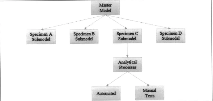
simulation that was simple and could be readily transferred to Quest employees for practical use and that it could be scalable to future modifications to the current system and to applications in future systems. Therefore the simulation was structured to be tiered and modular. Figure 4 below illustrates the overall architecture of the simulation model. And Figure 5 illustrates the master model, which calls for the sub-models.

aFgr 4

Figure 4: Simulation Model Architecture

(32)

nBuk input

Typ Submod

Pre-Anaoncal Equipment Resources

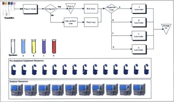
Figure 5: Master Simulation Model

The model is built such that the specimen flow can be followed from door to storage. The requisition element depicted in Figure 5 generates requisitions based on the arrival pattern

planned by

Quest.

The presort model simulates the processes performed to accept the requisition into the system and separate the specimens associated with each requisition. Once the specimens are loaded into the automated system through the input modules, the model sorts each specimen type and directs it to it corresponding sub-model. Each specimen sub-model simulates all the pre-analytical and analytical processes required and outputs the specimen to the storage module. As required by legal regulations, the specimens are stored for a period of 7 days prior to being disposed. This step was omitted from the model for simplicity and because each simulation run only covers two days. Various analyzers and pre-analytical equipment are used in multiple sub-models, therefore, they are defined at the master model level. These are depicted in the bottom two rows of Figure 5.

(33)

4.3 Performance Metrics and Data Sources

4.3.1 Performance Metrics

The following performance metrics were monitored for each simulation and will be further discussed in Chapter 5.

" Equipment queue size

" Equipment utilization

" Average cycle time for each specimen type

" Total specimens processed by each equipment (monitored for model validation only)

The metrics above directly relate to the goals of the simulation.

1. Verify the designed capacity of the automation system.

2. Study the sensitivity of the system to various disturbances.

3. Verify that the simulated load to the system is comparable to the experienced load in the

current manual system and the expected load in the automated system.

4.3.2 Data Sources

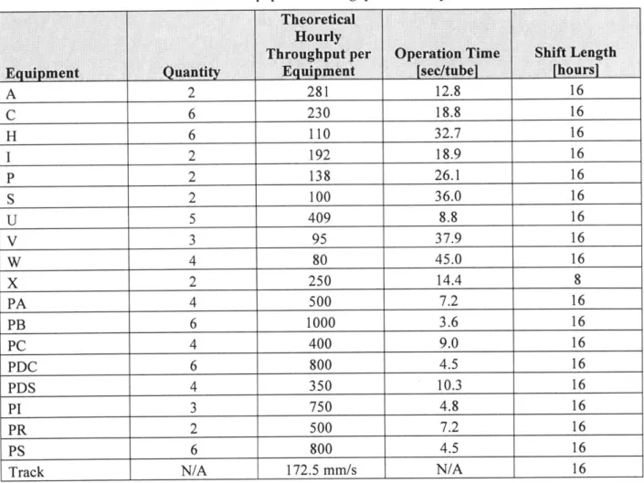
Beyond the process flow and the structure of the simulation, it was necessary to input various data based on Quest's current manually operated system and the design documents for the automated system. The first data input was the theoretical throughput for each equipment that is part of the automation system. Table 1 summarizes the throughput data of each analyzer and pre-analytical equipment. The pre-pre-analytical equipment is identified by a preceding letter "P".

(34)

Table 1: Equipment Throughput Summary Theoretical

Hourly

Throughput per Operation Time Shift Length

Equipment Quantity Equipment [see/tubeL [hours]

A 2 281 12.8 16 C 6 230 18.8 16 H 6 110 32.7 16 1 2 192 18.9 16 P 2 138 26.1 16 S 2 100 36.0 16 U 5 409 8.8 16 V 3 95 37.9 16 W 4 80 45.0 16 X 2 250 14.4 8 PA 4 500 7.2 16 PB 6 1000 3.6 16 PC 4 400 9.0 16 PDC 6 800 4.5 16 PDS 4 350 10.3 16 PI 3 750 4.8 16 PR 2 500 7.2 16 PS 6 800 4.5 16

Track N/A 172.5 mm/s N/A 16

The second data input is the arrival pattern of specimens into the system. This data is planned by Quest as part of scheduling the transportation of specimens from the collection sites to the

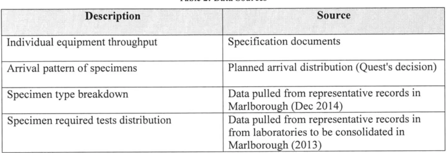
laboratory. The third is the number of specimens of each type as a percentage of the total number of specimens processed each day. And finally, the fourth input is the correlation of how many specimens are processed by multiple analyzers and which analyzers process them. Table 2 on the next page describes the source for the data used as input to the simulation.

(35)

Table 2: Data Sources

Dlescription Source

Individual equipment throughput Specification documents

Arrival pattern of specimens Planned arrival distribution (Quest's decision)

Specimen type breakdown Data pulled from representative records in

Marlborough (Dec 2014)

Specimen required tests distribution Data pulled from representative records in from laboratories to be consolidated in Marlborough (2013)

(36)

(37)

5 Simulation Results

5.1 Model Validation

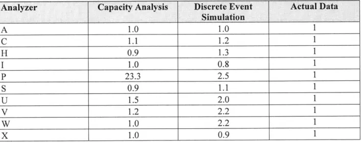
Prior to running all the scenarios described in the next section, it was necessary to validate the discrete event model against the real system. Since the automated system is not yet operational, the model was validated against two sources: the current manually operated system and a previously performed capacity analysis of the system. Due to differences in the process flow for the current system and the model, the only comparable data is the daily load experienced by each analyzer. The same is true for the capacity analysis of the system because it only accounted for overall load in each platform and not an actual process flow. Table 3 below compares the loads normalized to the actual data recorded over the period of one day. Taking into account the typical variation on demand experienced by Quest on a daily basis, a deviation of up to + 0.2 from the actual data is considered acceptable for the simulation results. The exception to this target is platform P, which has a cyclical demand and as such, it was sized to support the peak demand of 23x the demand on the sampled day.

Table 3: Original Model Daily Load Comparison

Analyzer Capacity Analysis Discrete Event Actual Data

Simulation A 1.0 1.0 C 1.1 1.2 H 0.9 1.3 1 1.0 0.8 P 23.3 2.5 S 0.9 1.1 U 1.5 2.0 V 1.2 2.2 W 1.0 2.2 X 1.0 0.9

(38)

As shown in Table 3, there were five different platforms that the discrete event simulation exceeded the allowable 0.2. Further investigation of this discrepancy revealed that the differences in the processes used for manual operations from the automated operations have a much larger impact than originally assumed.

The most impactful difference is the handling of specimens requiring to be processed by multiple testing platforms. In manual operations, prior to testing, the specimen is divided into multiple vials (aliquots) which then are simultaneously routed to the various departments/platforms to be tested. On the other hand, the automated system will not require this process and the specimens will be routed to each platform sequentially. In of itself, this difference should not impact the resulting daily load on each platform. However, this difference causes problems when comparing the two sets of data. When the specimen count is extracted from the Quest database, there is no way to discern between an original specimen and an aliquot. This in turn affects the flow

breakdown numbers that were used as input to the simulation as described in Chapter 4. The only way to truly correct the simulation will be to collect real data from the automated system when it becomes fully operational.

Although determining the true process flow breakdown of the automated system was not possible, the simulation parameters were adjusted to produce a load on each platform that was within the 0.2 range previously mentioned. Table 4 summarizes the results after the discrete event model's parameters were adjusted. This adjusted model was then used to evaluate the system and in all subsequent sensitivity analysis discussed herein.

Ultimately, further work is needed to properly match the exact flow of specimens through the simulation to the real system when it becomes operational. However, the current simulation is

(39)

adequate to evaluate the system capability to process the specimen daily demand. The

modifications described above result in a simulated daily demand for each analyzer that is within 20% of the daily demand recorded for the manual operations. As explained previously, this range is considered acceptable when compared to a single day of collected data due to the natural variation of demand for the laboratory. Since the simulation baseline is within the acceptable range to the collected data, the other scenarios discussed herein can be evaluated with

confidence.

Table 4: Adjusted Model Daily Load Comparison

Analyzer Capacity Analysis Discrete Event Actual Data

Simulation A 1.0 1.0 C 1.1 1.1 H 0.9 1.0 1 1.0 1.0 P 23.3 23.5 S 0.9 1.0 U 1.5 1.2 V 1.2 1.0 W 1.0 1.1 X 1.0 1.1 5.2 Scenarios

Before describing the simulation scenarios, it is worth to briefly describe Quest's plans for the automation system. There are two phases to the design. The first, which is herein referred to as the baseline, is currently being implemented. The second phase involves an increase in the system capacity to support a 20% increase in the daily specimen volume. The increase in capacity will be accomplished by adding units of pre-analytical equipment and analyzers. Table

(40)

Table 5: Phase 2 Capacity Increase

Equipment Quantity Increase

H 3 C P 1 PB PR PS S V W

Three parameters were varied to create each scenario: equipment efficiency, transport track speed, and equipment downtime. The equipment performance directly represents the throughput of each equipment and the scenarios included two variations: no change and 10% reduction. The transport speed also was varied with no change and a 10% reduction. And the equipment

downtime was varied between 0% and 10% downtime.

The simulation scenarios can then be divided between the two phases of the system design but with similar variations to the simulation parameters to evaluate the system sensitivity. An additional scenario was also simulated to evaluate the effect of an additional 10% increase in volume for a total 33% increase over the baseline.

(41)

* Phase 1 Design:

o Baseline: 100% equipment efficiency and transport speed, zero downtime o 90% equipment efficiency

o 90% transportation speed o 10% equipment downtime

o 90% equip. eff.; 90% trans. speed

o 90% equip. eff.; 10% equip. downtime o 90% trans. speed; 10% equip. downtime

o 90% equip. eff.; 90% trans. speed; 10% equip. downtime o 20% increase in volume with baseline design.

* Phase 2 Design

o 20% increase in volume

o 20% increase in volume; 90% equip. eff. o 20% increase in volume; 90% trans. speed o 20% increase in volume; 10% equip. downtime

o 20% increase in volume; 90% equip. eff.; 90% trans. speed o 20% increase in volume; 90% equip. eff.; 10% equip. downtime o 20% increase in volume; 90% trans. speed; 10% equip. downtime

o 20% increase in volume; 90% equip. eff.; 90% trans. speed; 10% equip. downtime o 33% increase in volume

(42)

5.3 Analysis Results and Key Findings

5.3.1 Phase 1 Design

Figure 6 shows the queue size at each analyzer over the simulated period of 48 hours. Although the number of specimens in queue for each analyzer varies over time, each analyzer's queue

reaches zero at approximately 24hr period. This is evidence that the system is able to process the entire daily specimen volume. It can be noted that there is a lag in the system for when each analyzer finishes the daily demand. This is mainly driven by the pre-analytical processes that are required for select analyzers and the travel time between processing equipment. Furthermore, Figure 7 shows that most analyzers are underutilized. The baseline results in Figure 6 and in Figure 7 show that the designed system is able to support the required daily specimen demand. It can be noted, however, that Analyzer H shows a relatively higher queue length in comparison to the other platforms, as well as 85% utilization. This is not a detriment to the system performance,

since Analyzer H can process the entire daily demand within 24hrs.

Baseline Results 1400 1200 1000 Z 800 _ 600 -400 200 0 0 6 12 18 24 30 36 42 48 SIMULATEDTIME [HR] -A -C H - -P S -U -V -W -X

Figure 6: Phase 1 Design - Baseline Results

(43)

Analyzer Utilization [Baseline]

85.1% 66.8% 66,4% 56.1% 45.4% 43.9% 3

E2.2%

C H I P S U V 90% 80% 70% 60% 50% 40% 30% 20% 10% 0%

Figure 7: Phase I Design - Baseline Utilization

Additionally, Figure 8 and Figure 9 show that the system is not affected by a 10% reduction in the track speed. And not surprisingly, a reduction in equipment efficiency by 10% has similar effect to 10% equipment downtime. Since the model does not include additional processes that remain manually operated, the average cycle times depicted in Figure 8 cannot be interpreted in absolute terms, but in relative terms from a sensitivity analysis of the system.

Furthermore, Analyzer H processes mainly specimen type B, and the effect of the reduction in system efficiency and increase in downtime can be seen in the cycle time increase in specimen B.

Since the automation track serves as the queue for all equipment, it was important to monitor the total queue size for the system. Figure 9 depicts the peak and average queue for the system in

each scenario of Phase 1. Since the storage buffers have a combined capacity of over 10,000 specimens, the system is able to handle the maximum queue for every simulated scenario.

43 29.1% 0.3% - I W X 21.0% I A

(44)

Figure 8: Phase 1 Design - Average Cycle Times Baseline Design 8000 6000 4000 00 2000 0 Max Queue I I

I

1 0 Avg Queue e 'V" 0 * o 13 0 4 - O J o 0 P 4 0 0 0 e O 0

Figure 9: Phase 1 Design - Total Queue Size

Analyzer H becomes unable to handle the daily demand under the combined effects of reducing the equipment efficiency by 10% and increasing the downtime to 10% and when the volume is increased by 20% to phase 2 levels without increasing capacity. The latter of the three is depicted 44 Baseline Design 160 cu 120 E 80 40 0

.o '01 oo coo % *'JO elo essv

%A I I..- I -- Specimen A -4*-Specimen B SSpecimen C -4+- Specimen D -0-Average

(45)

in Figure 10. These scenarios are equivalent to a reduction in equipment capacity of 20%, which drives the utilization of Analyzer H to approximately 105%. Since Analyzer H is only marginally over capacity in these three cases, the specimen backlog can be worked through by increasing the work shift by Ihr each day.

20% Increase in Volume Results

3000 2500 2000 1500 1000 500 0 6 12 18 24 30 36 42 48 SIMULATED TIME [HR] -A -C H -I -P S -U -V -W -X

Figure 10: Phase 1 Design - 20% Increase in Volume 5.3.2 Phase 2 Design

As previously described in Table 5, the Phase 2 design increases capacity various analyzers, including Analyzer H. This results in completely eliminating Analyzer H as a potential bottleneck of the system. In fact, the system design in Phase 2 has much excess capacity, as shown by the very low queues depicted in Figure 11. Furthermore, the utilization for Analyzer H is reduced to 70% with a 20% increase in volume, as shown in Figure 12.

(46)

Figure 11: Phase 2 Design - Baseline Results

Analyzer Utilization [Phase 2 Baseline]

80% 70.6% 70% 60% 59.1% 56.2% 54.0% 53.3% 53.0% 50% 40% 34.4% 30% 25.0% 27.4% 20% 10% 0.3% 0% 111 1 1 1 1 -I A C H I P S U V W X

Figure 12: Phase 2 Design - Baseline Utilization

In addition, although the various scenarios affected the maximum queue size when more than one disturbance is introduced, the average queue size and the average cycle times see very little change. Figure 13 and Figure 14 also show that the system can even support an additional 10%

46

Phase 2 Baseline Results

1000 900 800 700 L 600 LJ500 a 400 300 200 100 0 0 6 12 18 24 30 36 42 48 SIMULATED TIME [HR) S -U -V -W -X -A -C H -I --- P

(47)

increase in specimen volume (33% increase from Phase 1 baseline). In fact, the maximum queue

sizes shown in Figure 14 are even lower than in Phase 1.

Figure 13: Phase 2 Design - Average Cycle Times

High Volume Design 6000 4000 2000 0 Max Queue * Avg Queue '4 eel 14: s

Figure 14: Phase 2 Design - Total Queue Size

47

High Volume Design 160 120 E 80 40 0

9& 1&' & %)1 1 (0 9

-*- Spe cimen A --- Specimen B

,- Specimen C

--- Specimen D

(48)

(49)

6 Automation Transition

As mentioned previously in Chapter 2, the transition from manual into automated operations is happening in two steps. The first, being the physical installation of the automation equipment and physical connection of the analytical equipment to the automation system. The second step is to switch each analyzer from manual operations into automated operations. Since the system was designed such that any analyzer can be operated manually when necessary, the equipment is not required to remain idle between steps 1 and 2. Additionally, the transition is especially

challenging because it is happening at a lab that is currently fully operational in manual mode. In some cases, analyzers will need to be temporarily relocated to allow room for technicians to assemble and install the automation system prior to being placed in their final location and connected to the system. And every analyzer will be physically connected to the automation system.

All the movement of equipment while operating a diagnostics lab and maintaining full service to

clients and patients is cause for much concern for the project management team. Also, it is imperative that the transition happens with no negative impact to quality and service level to Quest's clients. Therefore, it is paramount to identify and mitigate all risks involved in such endeavor.

(50)

6.1 Methodology/Approach

A risk assessment was performed on the transition plan. And although it was mainly focused on the physical movement and installation of the analytical equipment, it can be easily transferred to the second step of the transition.

The overall methodology followed a typical risk assessment process, but modified to include the benefits of lessons learned during the transition efforts. Due to space constraints and the need to maintain normal operations within the lab, the analytical equipment can only be transitioned one at a time. This constraint provides an opportunity to use the lessons learned in the transition of one analyzer on the next one in line. The entire risk assessment process developed is listed below.

1. Brainstorm the risks associated with the transition of each equipment platform.

2. Score each risk based on its severity and probability of occurrence.

3. Calculate the overall risk for each equipment platform, accounting for lessons learned.

4. Prioritize risks and equipment platforms based on total risk scores.

5. Brainstorm mitigation measures.

6. Re-score each risk in light of the mitigation measures in place.

7. Update the overall risk based on the new scores.

(51)

6.1.1 Overall Risk Score Calculation

As mentioned in the last section, there is a need to include a factor in the risk score calculation to account for lessons learned. However, not all lessons are created equal. There are two types of lessons learned, and as such, there should be two different factors and/or two different ways to account for them.

One type of lessons learned covers lessons from different instances of the exact same equipment. For example, when an equipment platform has two analyzers, ordinarily the raw risk score would simply be multiplied by 2. However, since the equipment is being transitioned one at a time, the second equipment to be moved should have a reduced factor. It follows that if there is a third analyzer, it should be reduced even further due to the opportunities for lessons learned from each of the two analyzers that were transitioned before. Generalizing, the equation below can be formulated.

Kil = faa _eq.₁

i=1

Where:

Kpni - Platform lessons-learned factor

j

- Number of analyzers of the platform

faa - Additional analyzer factor

The second type of lessons learned covers lessons from transitioning a different platform before another is transitioned. This factor is directly related to platform's position in the transition sequence and can be summarized by the following equation.

Ki s = (seq-) eq. 2

Where:

Ksi - Sequence lessons-learned factor

(52)

Combining the two factors introduced above, the Overall Risk Score can be calculated for each equipment platform with the equation below.

n

RS = _{(SSi - PSi) -} _faa"j'i _-s

eq. 3

i=1 i=1

Where:

RS - Total risk score

SSi - Severity score for risk i PSi - Probability score for risk i

n - Number of risks for analyzer platform

6.2 Analysis Results and Key Findings

The entire purpose of the risk assessment scoring is to prioritize all risks that were identified during the brainstorming sessions. Table 6 effectively summarizes the total risk scores before and after the mitigation actions were executed. As with most risk assessments, the absolute scores are meaningless and should only be evaluated in relation to the scores of the other items in the risk assessment. Furthermore, items which scored below 500 points in the original risk

assessment were considered relatively low risk and low on the risk mitigation priority. As such, their risk assessment scores were unchanged after mitigation efforts were in place.

(53)

Table 6: Risk Scores Summary

Analyzer Risk Score Risk Score Post Mitigation

H (Qty 6, 6th to be transitioned) 1388 1127 V (Qty 2, 1st to be transitioned) 959 711 A (Qty 2, 4th to be transitioned) 880 714 W (Qty 4, 7th to be transitioned) 825 670 C (Qty 6, 10th to be transitioned 806 655 Hi (Qty 2, 6th to be transitioned) 802 651 BP (Qty 2, 11th to be transitioned) 602 489 U (Qty 5, 15th to be transitioned) 574 466

I

(Qty 2, 13th to be transitioned) 532 432 S (Qty 2, 12th to be transitioned) 493 493 P (Qty 2, 5th to be transitioned) 402 402 D (Qty 2, 8th to be transitioned) 311 311 Vi (Qty 2, 2nd to be transitioned) 307 307 B (Qty 2, 9th to be transitioned) 299 299 X (Qty 2, 14th to be transitioned) 242 242 Ii (Qty 1, 3rd to be transitioned) 214 214

The most important results of a risk assessment are the mitigation actions that are identified in the process. The mitigation steps can be divided into 2 main categories: Transition best practices and Backup operations. All mitigation actions taken are listed in Table 7.

(54)

Table 7: Risk Mitigation Actions

Transition Best Practices Back-up Operations

Coordinate with vendors to be on-site during Install additional analyzers temporarily to transitioning to ensure fast response to any provide back-up to Platform H.

issues

Pre-check all connections prior to Vi will serve as additional back-up for

transitioning equipment. Platform V.

Establish strict time limits to resolve issues or Install additional analyzers temporarily to return to original configuration while issue is provide back-up to Platform A.

resolved

Plan transition efforts for low volume times, Keep supporting satellite locations on standby

i.e. nights and weekends to provide operations back-up when

necessary. Stagger transition between platforms to avoid

an entire platform being down at one time.

The transition process was still in progress at the conclusion of this project. More specifically, it was approximately 20% complete, meaning that Analyzers V, Vi, Ii, A, and P had been

completely transitioned into their final positions and were again operational in manual mode awaiting the completion of the transition prior to being transitioned to automated operations. Although these analyzers were the least complex for the transition, lessons learned from analyzers V and Vi were being applied to the transition of the later analyzers, reducing the transition time and the number of unexpected issues. Furthermore, the mitigation actions listed in Table 7 were successfully in place at the time of the transitions.

Although the learning factors included in the risk assessment could not be verified quantitatively, the application of lessons learned and the increasing speed that each analyzer was being

transitioned qualitatively support the methodology developed herein.