Response of the convecting high-latitude F layer to a powerful HF wave

(1)

HAL Id: hal-00316332

https://hal.archives-ouvertes.fr/hal-00316332

Submitted on 1 Jan 1997

HAL is a multi-disciplinary open access archive for the deposit and dissemination of sci-entific research documents, whether they are pub-lished or not. The documents may come from teaching and research institutions in France or abroad, or from public or private research centers.

L’archive ouverte pluridisciplinaire HAL, est destinée au dépôt et à la diffusion de documents scientifiques de niveau recherche, publiés ou non, émanant des établissements d’enseignement et de recherche français ou étrangers, des laboratoires publics ou privés.

Response of the convecting high-latitude F layer to a

powerful HF wave

G. I. Mingaleva, V. S. Mingalev

To cite this version:

G. I. Mingaleva, V. S. Mingalev. Response of the convecting high-latitude F layer to a powerful HF wave. Annales Geophysicae, European Geosciences Union, 1997, 15 (10), pp.1291-1300. �hal-00316332�

(2)

Ann. Geophysicae 15, 1291—1300 (1997) ( EGS — Springer-Verlag 1997

Response of the convecting high-latitude F layer

to a powerful HF wave

G. I. Mingaleva, V. S. Mingalev

Polar Geophysical Institute, Fersman Str. 14, Apatity, Murmansk Region 184200, Russia Received: 17 November 1994/Revised: 8 January 1996/Accepted 5 February 1996

Abstract. A numerical model of the high-latitude iono-sphere, which takes into account the convection of the ionospheric plasma, has been developed and utilized to simulate the F-layer response at auroral latitudes to high-power radio waves. The model produces the time vari-ations of the electron density, positive ion velocity, and ion and electron temperature profiles within a magnetic field tube carried over an ionospheric heater by the con-vection electric field. The simulations have been per-formed for the point with the geographic coordinates of the ionospheric HF heating facility near Tromso, Norway, when it is located near the midnight magnetic meridian. The calculations have been made for equinox, at high-solar-activity, and low-geomagnetic-activity conditions. The results indicate that significant variations of the elec-tron temperature, positive ion velocity, and elecelec-tron den-sity profiles can be produced by HF heating in the convecting high-latitude F layer.

1 Introduction

The modification of the D and E regions of the auroral ionosphere by HF heating has been extensively studied in recent years both experimentally (Kapustin et al., 1977; Stubbe et al., 1981; Barr et al., 1986; Rietveld et al., 1989) and theoretically (Stubbe and Kopka, 1977; Barr and Stubbe, 1984), and these studies have been a great success. Many interesting results concerning the auroral lower-ionosphere modification by a powerful HF wave were obtained. The ionospheric HF heating facility near Tromso, Norway is successfully utilized now for these experimental studies.

Nevertheless, the studies just mentioned deal with the lower ionosphere (D and lower E regions) only. The ma-jority of theoretical and numerical investigations of the

Correspondence to: V. S. Mingalev

F region have been mainly directed to study the mid-latitude ionosphere (Gurevich, 1967; Meltz and LeLevier, 1970; Savelev and Ivanov, 1976; Perkins and Roble, 1978; Mantas et al., 1981; Bernhardt and Duncan, 1982; Mul-drew, 1986; Newman et al., 1988; Blaunshtein et al., 1992; Vas’kov et al., 1993). This is essentially because of the location of the earlier experimental facilities in the mid-latitudes, for example, Platteville, Arecibo, Gorky.

However, it is known that the high-latitude ionosphere possesses some specific features which are unusual for the mid-latitude ionosphere. In particular, the ionospheric plasma at F-layer altitudes convects at high latitudes. The plasma convection in the polar ionosphere is mainly in-duced by magnetospheric electric fields. The convection flow over the polar region can differ considerably from the ionospheric plasma flow at mid-latitudes. The latter flow has a strong tendency to corotate with the earth. There-fore, at mid-latitudes a ground-based ionospheric heater can affect a heated plasma volume for very long time. On the other hand, at high latitudes a restriction of the dura-tion of a powerful HF wave effect on a heated plasma volume does exist. The attainable duration depends on heater parameters and geophysical conditions. For example, for the Tromso heating facility, the half-power heated-plasma-volume diameter is 75 km at an altitude of 300 km. The available drift velocity of the ionospheric plasma at F2-layer altitudes is about 500 m/s. Hence, the maximum duration of a powerful HF wave effect is about 150 s near the F2-layer peak, and thus the ionospheric heater cannot affect the same heated plasma volume dur-ing a time longer than the magnitude pointed out. This is the principal distinction between mid- and high-latitude ionospheres with respect to the F-layer modification by a powerful HF wave.

Many details of the response of the high-latitude F layer to high-power radio waves have the potential to be investigated by using numerical models. To date there have been very few numerical studies of the high-latitude F-layer modification by a powerful HF wave. The numer-ical model of the polar ionosphere F region heated by high-power, high-frequency waves has been developed by

(3)

Shoucri et al. (1984); this paper also presented the results of simulation of the modifications produced by a powerful HF wave in the F region of a quiet (low solar cycle) polar ionosphere. The model of Shoucri et al. (1984) contains some simplifications and restrictions; in particular, an idealized vertical magnetic field parallel to the ionospheric density gradient is used. Moreover, the model does not take into consideration the convection of the ionospheric plasma. Nevertheless, this model has been used to study the time evolution of the density depressions formed at the reflection height of HF waves propagating in a daytime ionosphere (Hansen et al., 1989).

The purpose of the present study is to develop an alternative numerical model of the high-latitude F layer which takes into account the geomagnetic field declina-tion and the convecdeclina-tion of the ionospheric plasma. More-over, we make an attempt to predict the time variations of the electron density, positive ion velocity, and ion and electron temperature profiles during the disturbance caused by HF heating for one case eventual for the iono-spheric heater near Tromso, Norway.

2 The model of the heated F layer

Over the last year we have been developing a numerical model of the high-latitude F region which can be affected by a powerful HF wave. The model allows us to study changes of ionospheric quantities produced by HF heat-ing at F-layer altitudes.

2.1 Basic principles

Our model employs the idea put forward by Knudsen (1974) which was then pursued quantitatively by Knudsen

et al. (1977). The ionospheric plasma at F-layer altitudes

may be considered attached to the magnetic field lines, which are convecting over the polar region. A plasma transport along a magnetic field line may be rather arbi-trary. A perpendicular (to the magnetic field) plasma flow is strongly controlled by the convection electric field. In general, the ionospheric plasma motion at F-layer alti-tudes may be separated into two flows: first, the plasma motion parallel to the magnetic field; second, the plasma drift in the direction orthogonal to the magnetic field. The latter drift may be easily obtained by using the model of the convection electric field. To describe the parallel plasma transport it is convenient to consider a magnetic field tube of the F-layer plasma carried around the polar region by the convection electric field.

The basic principles described above are utilized by our numerical model of the heated F layer. In the present study we consider a part of a magnetic field tube of ionospheric plasma at distances from the earth along the magnetic field line between 100 and 700 km. The point of view taken, is that the part of the magnetic field tube of plasma is carried over an ionospheric heater by the con-vection electric field.

At the present time, there are several theoretical and empirical models that describe the plasma convection in

the high-latitude ionosphere (Sojka et al., 1986, and refer-ences therein). The plasma convection pattern varies markedly with the interplanetary magnetic field (IMF). For southward IMF, the pattern has two vortex cells with antisunward flow over the polar cap and return flow equatorward of the auroral oval. The results of the simula-tion to be presented in this paper were obtained for southward IMF by using pattern B of the empirical con-vection models of Heppner (1977), which is the steady nonsubstorm convection pattern. It is known that the flow paths (or the convection trajectories), around which the magnetic field lines are carried over the polar region, are closed for a steady convection pattern. From the plasma convection pattern used, we obtain the convection traject-ory, which intersects the F-layer volume illuminated by the heating facility at Ramfjordmoen near Tromso, Norway, when it is located near the midnight magnetic meridian, and calculate the plasma drift velocity along the convection trajectory.

In the model calculations of the F-layer modification by a powerful HF wave, the temporal history of the plasma in the given magnetic field tube is traced during its movement along the considered convection trajectory not far from the ionospheric heater. For the considered con-vection trajectory, we obtain variations of ionospheric quantities with time (along the trajectory), with the rela-tion between the distance along the trajectory and time containing the calculated plasma drift velocity. The part of the considered convection trajectory, around which the plasma tube was carried in the numerical simulation, is shown in Fig. 1.

2.2 Transport equations

We consider a relative frame of reference moving together with the plasma tube along the convection trajectory. It is supposed that the origin of coordinates moves so that it is retained on the earth’s surface, and one of the axes (axis h) of the reference frame is directed upwards along the mag-netic field line. As pointed out previously, the ionospheric plasma at F-layer altitudes is attached to the magnetic field line. Therefore, the movement of plasma in a direc-tion perpendicular to the axis h is absent at F-layer alti-tudes. This detail provides the simplifications of transport equations of ionospheric plasma in the relative frame of reference.

The model F-layer plasma is assumed to consist of electrons and positively, singly charged atomic oxygen ions; other ionic species are neglected. It is well known that the positive O` ions are dominant above approxi-mately 200 km in the polar ionosphere. The behaviour of the ionospheric plasma in the part of the magnetic field tube, moving along a convection trajectory through a neu-tral atmosphere, may be described by transport equations. Our model allows us to simulate the temporal history of both the dynamics and the temperature regime of ion and electron gases in the magnetic field tube. The profiles, against distance from the earth along the geomagnetic field line of ionospheric quantities, are ob-tained by solving the appropriate system of transport

, (4) where N is the O` ion number density (which is supposed to be equal to electron concentration N% at the F-layer altitudes); » is the parallel (to the magnetic field) compo-nent of the positive ion velocity; q is the photoionization rate; q% is the production rate due to auroral electron bombardment; q1 is the production rate due to auroral proton bombardment; l is the positive-ion loss rate (taking into account the chemical reactions O`#O2PO`2#O, O`#N2PNO`#N, O`2#ePO#O, and NO`# ePN#O); m* is the positive ion mass; k is Boltzmann’s constant; ¹* and ¹% are the ion and electron temperatures, respectively, g is the acceleration due to the gravity; I is the magnetic field dip angle; 1/q*/ is the collision frequency between ion and neutral particles of type n; º/ is the parallel component of velocity of neutral particles of type n; M"3/2 kN; c"5/3; v is the parallel component of electron velocity (which is determined from the equation for parallel current); k is the ion viscosity coefficient; j* and j% are the ion and electron thermal conductivity coefficients, respectively; Qr, Q%, Q1, and Q& are the elec-tron heat rates due to photoionization, auroral elecelec-tron bombardment, auroral proton bombardment, and HF heating, respectively; and ¸3, ¸7, ¸%, and ¸& are the elec-tron cooling rates due to rotational excitation of mole-cules O2 and N2, vibrational excitation of molemole-cules O2 and N2, electronic excitation of atoms O, and fine

structure excitation of atoms O, respectively. The quantit-ies on the right-hand sides of Eqs. 3 and 4, denoted by Pab, describe the rates of change of energy of particles of type a as a result of elastic collisions with particles of type b. These quantities contain the terms proportional to the species-flow velocity differences squared which describe the frictional heating of ionospheric plasma due to both the convection electric field and the neutral wind.

2.3 Model parameters

Concrete expressions must be given to a number of param-eters that appear in the equation system of Eqs. 1—4, for the model fulfilment. Expressions of plasma parameters, such as viscosity coefficient, thermal-conductivity coeffi-cients, collision frequencies, and ion and electron rates of change of energy due to elastic collisions, are well known; they are the same as in our previous models (Mingaleva

et al., 1982a; Mingaleva et al., 1982b; Mingalev et al., 1984;

Mingalev et al., 1988), and very similar to those utilized by models of Stubbe (1970), Schunk and Sojka (1982), and Schunk et al. (1986).

As was noted earlier, the results of calculations to be presented in this paper were obtained for nighttime. Gen-erally, our model allows us to simulate changes of the ionospheric F layer produced by HF heating for arbitrary time. Therefore, the photoionization sources included in the model are solar EUV photons, both direct and reso-nantly scattered. The total photoionization rates from both the direct and the resonantly scattered photons are calculated by the method analogous to that utilized by Knudsen et al. (1977). Also, ionization sources included in the model are soft electron and proton precipitations. The production rate due to soft electron bombardment as a function of height is calculated by the method analogous to the semiempirical method of Rees (1963). Altitude profiles of the production rate due to soft proton bombardment are calculated after the method given by Chamberlain (1961) and developed by Eather and Burrows (1966).

Energy-dependent rate coefficients for chemical reac-tions included in the model were taken from Timothy

et al. (1972) and St.-Maurice and Torr (1978). The electron

heat rate due to photoionization Qr is assumed to be the product of the photoionization rate q and a heating effi-ciency parametere

Qr"e·q, (5) with heating efficiencies, both local and nonlocal, having been taken into account. Altitudinal dependences of these heating efficiencies were taken from Stubbe (1970) and Hanson and Johnson (1961). By analogy with Eq. 5, the electron heat rates due to auroral electron and proton bombardments are calculated, and appropriate heating-efficiency parameters are utilized which are taken from our previous model (Mingaleva et al., 1982b). The expres-sions of the electron cooling rates due to inelastic colli-sions with neutral molecules and atoms were taken from Stubbe and Varnum (1972).

(5)

2.4 Source of HF heating

The electron heat rate due to HF heating, Q& used in Eq. 4, is given by Eq. 7 in Blaunshtein et al. (1992),

Q&"Q.&exp

G

!b2

A

N!NR

NR

B

2

H

, (6)

where Q.& is the maximum value of the electron heat rate due to HF heating, parameter b characterizes the ‘‘half-width’’ of the source function, and NR is the electron hybrid resonance value of electron concentration.

From Eq. 6 it follows that the electron heat rate Q& de-pends nonlinearly on the incident wave frequency f0, and achieves the maximum value when the wave frequency

f0 is equal to the frequency of the electron hybrid

reso-nance, namely,

f0"( f 2N#f 2H)1@2, (7) where fN is the plasma frequency, given by the well-known formula,

fN"21n

A

Ne2

e0m%

B

1@2, (8)

fH is the electron cyclotron frequency, namely, fH"21n

eB

m%. (9)

Here e and m% are, respectively, the charge and mass of electron, B is the magnitude of magnetic field, e0 is the dielectric constant of free space. The electron hybrid reso-nance value of electron concentration NR may be obtained from Eq. 7 by using the relation given by Eq. 8. It follows that

NR"4n2e0m%e2 ( f20!f 2H). (10) It can be seen from relation in Eq. 10 that NR is less than the value of electron concentration corresponding to the plasma resonance, which can be expressed by the relation

N0"4n2e0m%e2 f20. (11) Therefore, the electron hybrid resonance height is less than the plasma resonance height in the regular F layer. Hence, the maximum energy absorption from the power-ful HF wave, described by Eq. 6, is to occur at a lower height than the expected reflection height of the HF wave.

It should be emphasized that the electron heating, described by Eq. 6, is possible when the transmitter oper-ates at a frequency which is greater than the F-layer critical frequency. Indeed, the maximum value of the plasma frequency fN, present in the relation given in Eq. 7, coincides with the F-layer critical frequency. Due to pres-ence of f2H in Eq. 7, the maximum value of the wave frequency f0, at which the transmitter operates, is greater than the F-layer critical frequency.

2.5 Model inputs

In general, our model can be employed for the simulation of the ionospheric plasma changes produced by powerful HF waves for an arbitrary location of an ionospheric heater. Besides, in the model calculations a magnetic field tube moving along a convection trajectory can be dis-placed for a rather long distance during a considered time. Therefore, some of the input parameters of the model must be given as global inputs. These global input param-eters can be distinct in various modeled situations. The results of calculations in what follows were obtained for one set of global input parameters.

The neutral atmosphere was assumed to consist of the species O, O2, and N2. The concentrations of the neutral species and the neutral-gas temperature were calculated from the empirical model of Jacchia (1977).

Our neutral-wind pattern is a combination of theoret-ical and empirtheoret-ical models. Altitudinal dependences of zonal and meridional components of the neutral wind were derived from model simulations performed by Min-galev (1979). These dependences were approximated by analytical expressions which contain the magnitudes of zonal and meridional components of the neutral wind at fixed altitude. The latter two magnitudes as functions of latitude and longitude were taken from an empirical model of the neutral wind. In the simulations of the present paper, the horizontal distribution of the neutral wind at 300 km is taken from Meriwether et al. (1973). In the model simulation, the horizontal components of vel-ocity of neutral particles are assumed to be identical for various neutral species. The vertical motion of neutral gas is supposed to be absent. The quantity on the right-hand side of Eq. 2, denoted by º/, is the parallel (to the mag-netic field) component of the neutral wind in the moving frame of reference.

Our model takes into consideration both electron and proton precipitations which act as an ionization source and as a source of heating for the electron gas. Spatial configurations of electron and proton precipitation zones and intensities, and average energies of precipitating elec-trons and protons were chosen as consistent with the statistical model of Hardy et al. (1989).

2.6 Solution of equations

The transport equations (Eqs. 1—4) form the system of four coupled nonlinear partial differential equations whose solution must be obtained numerically. To pose a rigor-ous mathematical problem, a set of boundary conditions must be formulated.

At the lower boundary (h"100 km), the concentration of positive ions is determined from the condition of the chemical equilibrium; the positive-ion velocity is given as a solution of the simplified momentum equation without accelerational and viscous terms; ion and electron tem-peratures are assumed to be equal to the neutral-gas temperature. At the upper boundary (h"700 km), the concentration of positive ions is given at each time step, as it is calculated from the continuity equation in which the

(6)

time derivative is expressed in the finite difference form, with other terms having been calculated using the value of the positive-ion concentration from the previous time step. Instead of », ¹*, and ¹%, the values of gradients L»/Lh, L¹*/Lh, and L¹%/Lh as a functions of time (along the trajectory) are given at the upper boundary. Through-out this paper, the latter gradients at the upper boundary are assumed to remain unchanged, namely,

L»

Lh"0, L¹*Lh"L¹%Lh"0.4 K/km. (12) In our computations we reduce the nonlinear tions (1—4) to a system of linear partial differential equa-tions, by calculating the coefficients of equations using the values of unknown quantities from the previous time step. The linear partial differential equations, obtained in such a way, are expressed in the finite-differences form using fully implicit methods. The resulting system of linear alge-braic equations is solved at each time step, and profiles of the unknown quantities are obtained.

3 Results and discussion

In the numerical simulation, a magnetic field tube of plasma is tracked as it moves along a convection trajec-tory through a moving neutral atmosphere. As was noted in Sect. 2.5, a magnetic field tube of plasma can be dis-placed for a rather long distance during a considered time. Neutral atmosphere parameters and other inputs to the model can be significantly different at distinct points of a convection trajectory. Therefore, it may be expected that ionospheric quantities, obtained by solving the system of transport equations, vary along a convection trajectory under natural conditions without a powerful HF wave effect. Initially, we are interested in examining variations of ionospheric quantities along the convection trajectory caused by a natural spatial inhomogeneity of the iono-sphere.

3.1 Unheated trajectory variations

As a field tube of plasma moves along a given convection trajectory, it is subjected to different physical and chem-ical processes at different times. Also, at a given time, the plasma in the field tube can be influenced by different chemical and transport processes at different altitudes. It may be recalled that convection trajectories, around which field tubes are carried over the polar region, are closed for steady convection patterns to which the convection model used belongs. For a closed convection trajectory, we solve the transport equations (Eqs. 1—4) successively at each time step, and obtain variations of calculated profiles with time (along the trajectory) until the profiles become re-peatable. Usually, no more than two complete traversals of a convection trajectory are necessary before calculated profiles start to repeat. A repeatable profile variation is assumed to be a steady distribution of ionospheric quan-tities along a given convection trajectory at fixed universal time (UT).

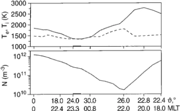
Our model can describe different combinations of solar cycle, geomagnetic activity level, and season. For the present study, the calculations were performed for equi-nox (31 March) and high solar activity (F10.7"230) con-ditions under low geomagnetic activity (Kp"0). The steady distribution of the ionospheric quantities, along the part of the convection trajectory presented in Fig. 1, at level h"300 km is shown in Fig. 2. It can be seen that the electron and ion temperatures and the electron concentra-tion are considerably different in distinct points of the convection trajectory under natural conditions without a powerful HF wave effect. It may be expected that the considered convection trajectory crosses the main iono-spheric trough in the evening sector. It turns out that the calculated electron concentration displays the deep min-imum in this sector. The ion temperature known to be mainly controlled by the convection electric field is en-hanced in the region where the electron-concentration minimum occurs. The minimal value of the electron tem-perature lies near the point which is most distant from the sun. Undoubtedly, the developed mathematical model produces some high-latitude ionosphere features known to be observed in the F layer under natural conditions without a powerful HF wave effect.

Fig. 1. The part of the convection trajectory around which the magnetic field tube of plasma is carried in the numerical simulation.

Arrows on the trajectory indicate the direction of the convection

flow. Locations of the plasma tube are labelled for 0, 20, and 1500 s after turn on of a power HF wave

Fig. 2. The variations along the part of the convection trajectory, presented in Fig. 1, (top) of ¹% (solid line) and ¹* (dashed line) in absolute degrees, and (bottom) of N in m~3 at level h"300 km under natural conditons without HF heating. Coordinates (mag-netic colatitude0and MLT) for some locations on the convection trajectory are pointed out near the horizontal axis

(7)

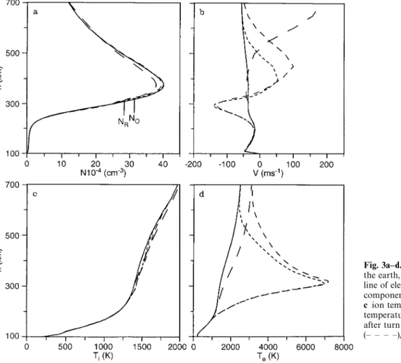
Fig. 3a–d. Profiles versus distance from the earth, a along the geomagnetic field line of electron concentration, b parallel component of the positive ion velocity, c ion temperature, d electron

temperature, at four distinct moments after turn on: 0 (——), 10 (- - - -), 20 (— — — —), and 100 (— —) s

It is obvious from results presented, that to obtain the pure HF heating effect by solving the system of transport equations, we must take into account the variations caused by a natural spatial inhomogeneity of the iono-sphere, which may be appreciable in the high-latitude F region. The latter variations can not be produced by numerical models, neglecting the convection of the iono-spheric plasma, in particular, the model of Shoucri et al. (1984).

3.2 Response to HF heating

In the present subsection we consider the variations of ionospheric quantities produced by a powerful HF wave along the chosen convection trajectory not far from the ionospheric heater. The same geophysical conditions as in previous subsection are considered. So far as geomagnetic activity is assumed to be low (Kp"0), the electron and proton precipitations, taken into account by our numer-ical model, exist poleward of the location of the HF heating facility imposed in this study. Hence, particle precipitations are absent during the action of a powerful HF wave on a magnetic field tube of plasma. The duration of the latter action, as was evaluated in the introduction, must be restricted. We therefore assume that the iono-spheric HF heater is turned on, and operates for 20 s. We suppose that a high-power HF wave is turned on when the

considered magnetic field tube is situated over the iono-spheric heater. Thus, the time variations of the electron density, positive-ion velocity, and ion and electron tem-perature profiles in the high-latitude F layer following the turning on of a powerful 20-s square HF pulse are simulated. We consider the temporal history of the iono-spheric plasma in the magnetic field tube during the peri-od of 1500 s. This periperi-od is sufficient for the magnetic field tube to be displaced for a distance of 630 km from the HF heater. The displacement of the plasma tube correspond-ing to the period pointed out is shown in Fig. 1 by a solid line and in Fig. 2 by a thick line.

The effective radiated power (ERP) is connected with the effective absorbed power (EAP) by the formula

EAP"gERP, (13)

whereg is the coefficient characterizing the fraction of the energy of the powerful HF wave deposited in the ambient electron gas and lost for its heating. The maximum value of the electron heat rate Q.& used in Eq. 6 depends on the EAP, which is assumed to be 60 MW. We assume that the ionospheric heater operates at the frequency f0"5 MHz._{Figure 3 presents calculated profiles of electron} con-centration, the parallel component of the positive ion velocity, and ion and electron temperatures at distinct moments after the HF heater is turned on. From Fig. 3d we see the great increase in ¹% near 300 km, when HF

(8)

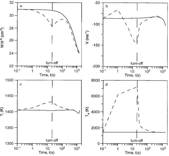
Fig. 4. a The time variations of electron concentration, b parallel component of the positive ion velocity, c ion temperature, d electron temperature, at level

h"316 km after turn-on of the HF

heater (dashed line). Solid lines present the ‘‘unheated’’ variations

heating operates. The peak value of ¹% is approximately 7300 K. After the HF heater is turned off, ¹% decreases rapidly due to elastic and inelastic collisions between electrons and other particles of ionospheric plasma which are taken into account by the heat-conduction equation of electron gas. The increase in ¹* is not considerable (Fig. 3c); therefore, the positive ion loss rate l, which is present in the continuity equation (1), does not change essentially at the F2-layer level during the perturbation caused by HF heating. The slight increase in ¹* is condi-tioned by two mechanisms. Firstly, ¹* increases due to the frictional heating conditioned by the enhancement of the difference between flow velocities of ions and the neutral gas. In fact, from Fig. 3b we see the significant changes in the positive-ion velocity profiles after the HF heater is turned on. As a consequence of these changes, the fric-tional heating, controlled by quantities proporfric-tional the term (»!ºn)2, occurs. Secondly, ¹* tends to rise due to elastic collisions between ions and electrons which are considerably heated by HF waves. However, it should be emphasized that the latter mechanism is much more slight than the former one. The fact is that the collision fre-quency of ions with electrons is considerably less than the collision frequency of ions with neutral particles at the F2 peak under the conditions of the present study. Conse-quently, there is no time for the perceptible enhancement of the ion gas temperature due to the second mechanism, before the strong increase in the electron temperature has ended. As a consequence of the great increase in ¹%, the

upward and downward ionospheric plasma fluxes arise from the level where the electron temperature peak is located.

From Fig. 3a we can see that the energy input from the powerful HF wave results in visible changes of the elec-tron-concentration profile. The remarkable feature is the variation of the electron concentration, not only near the level of maximum energy absorption from the powerful HF wave, but also near the F-region peak. This is a conse-quence of the specific ionospheric plasma fluxes caused by the great increase in ¹%._{The time variations of the computed ionospheric} quantities at levels of maximum energy input from the powerful HF wave and of the F-layer peak are presented in Figs. 4 and 5, respectively. It is seen from the results presented that the disturbance caused by a powerful 20-s HF pulse continues for about 5 min at the level of max-imum energy absorption from the HF wave. The differ-ence between heated quantities and unheated quantities achieves a peak at t"20 s, at level h"316 km, when the HF heater is turned off.

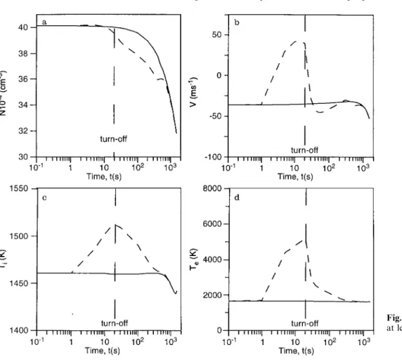
It should be emphasized that the disturbance caused by a powerful 20-s HF pulse continues for about 20 min at the level of the F-region peak. We can see that differ-ences between the heated ¹* and ¹% and the unheated values again have a maximum at t+ 20 s. However, the difference between the heated and unheated electron con-centrations is maximal at a much later time. The heated electron concentration is less than the unheated one: their

(9)

Fig. 5. The same as in Fig. 4 but at level h"380 km

difference can be more than 5%. Thus, the character-istic time for electron concentration changes caused by HF heating is greater than the time constants for ion and electron temperature changes near the F-region peak.

As mentioned, the duration of the disturbance caused by a powerful 20-s HF pulse continues for about 20 min at the F2-layer levels. It is obvious that the duration of the period of the ionospheric recovery after the HF heating depends on the values of ionospheric and neutral-gas quantities which take place along the convection trajec-tory considered. The latter quantities, as is seen from Fig. 2, may be significantly different in distinct sectors of the polar region. Therefore, it may be expected that the duration of the period of the ionospheric recovery after a powerful HF pulse will be different for distinct locations of an ionospheric heater and geophysical conditions un-der consiun-deration. However, we do not examine this ques-tion in the present paper, the problem being the subject of a future study.

From Eq. 6 it follows that the height of the maximum value of the electron heat rate due to HF heating depends on the electron concentration profile. As a consequence of a visible decrease in the F-region-peak electron concentra-tion after the HF heater is turned on, the height of the maximum energy input from the powerful HF wave be-gins to rise. Indeed, it is seen from Fig. 3a that the electron concentration begins to drop after the turning on of the HF heater above approximately 300 km at fixed altitudes.

Therefore, the height corresponding to the electron hybrid resonance value of the electron concentration, denoted by

NR, begins to rise. It is seen from results presented (Fig. 3a)

that the displacement of this height during the 20-s HF pulse reaches nearly 20 km. The heights of electron tem-perature peak at t"10 and t"20 s differ slightly for the same reason (Fig. 3d).

It is now generally understood that the energy absorp-tion of a powerful HF wave in the ionosphere can take place due to various linear and nonlinear processes. These processes include ohmic heating, excitation of plasma waves and ion waves by ponderomotive forces, origin of parametric and self-focusing instabilities, generation of field-aligned irregularities, origin of fast electrons, and others. A large fraction of the energy of the powerful HF wave is absorbed by electron gas, ultimately, by various heating channels [see Journal of Atmospheric and Terres-trial Physics, 44(12), 1982; also Radio Science, 9(11), 1974]. It should be emphasized that the purpose of this study is not to examine various electron heating channels, but rather to investigate how the absorbed energy of HF wave influences the behavior of the ionospheric quantities com-puted by a mathematical model taking into account the convection of the ionospheric plasma at high latitudes. In the present paper we make use of the expression of the electron heat rate due to HF heating, derived by Blaun-shtein et al. (1992). We shall not repeat earlier substanti-ations of its derivation (Blaunstein et al., 1992; Vas’kov

(10)

We make calculations for the case in which the effective absorbed power is equal to 60 MW. One would think that this magnitude is unattainable, but in fact the existing HF heating facilities can have effective radiated powers which are much greater than this magnitude. For example, the ionospheric HF heating facility near Tromso may achieve an effective radiated power up to 300 MW. Therefore, it seems to us that the chosen magnitude (60 MW) may be acceptable as an appropriate assumption of the effective absorbed power. Moreover, magnitudes still greater than ours have been used in simulations by other authors (Blaunstein et al., 1992; Vas’kov et al., 1993). Thus, our calculations may be considered as a prediction of the behavior of the convecting high-latitude ionosphere modi-fied by a high-power radio transmitter.

4 Conclusions

Principal distinctions between mid- and high-latitude ionospheres, as for the F-layer modification by a powerful HF wave, have been analyzed. It was established that the taking into consideration of plasma convection ought to result in some original features. First, the duration of a powerful HF wave effect on a heated volume of plasma, can not be unlimited. Second, the volume of plasma, disturbed by a powerful HF wave, can abandon the region illuminated by an ionospheric heater and be displaced for a long distance from the HF heating transmitter. Third, variations of ionospheric quantities produced by a power-ful HF wave are added to those caused by a natural spatial inhomogeneity of ionosphere. To obtain the pure HF heating effect one must subtract natural variations which may be significant in the high-latitude F region. The original features pointed out must be taken into account by numerical simulations of the high-latitude ionosphere’s response to high-power radio waves.

A mathematical model of the high-latitude F layer, which can be affected by a powerful HF wave, has been developed. In the model calculations the temporal history is traced of the ionospheric plasma in the part of the magnetic field tube, moving along a convection trajectory through a neutral atmosphere over an ionospheric heater. The model is based on the numerical solution of the appropriate system of transport equations for ionospheric plasma. The equations provide for field-aligned ion trans-port, EUV solar radiation, energy-dependent chemical reactions, frictional force between ions and neutrals, accel-erational and viscous forces of ion gas, thermal conduc-tions of ion and electron gases, heating due to ion-neutral friction, Joule heating due to solar EUV photons and powerful HF wave, and electron energy losses due to elastic and inelastic collisions. The geomagnetic-field de-clination and the ionospheric plasma drift caused by the convection electric field are taken into account, unlike in the previous model of Shoucri et al. (1984).

The mathematical model developed has been utilized to simulate the variations of ionospheric quantities under natural conditions without a powerful HF wave effect. The calculations have been made for equinox at high-solar-activity and low-geomagnetic-activity conditions for

the convection trajectory which lies across the location of the ionospheric heater near Tromso, Norway, when it is situated near the midnight magnetic meridian. It was found that considerable variations of the electron concen-tration and the electron and ion temperatures may take place in the polar ionosphere under natural conditions without HF heating. Obtained spatial inhomogeneity of the ionospheric F layer must be taken into account under the simulation of the ionospheric variations, produced by a powerful HF wave, and the periods of the ionospheric recovery after the HF heating.

The effect of the heating of a powerful HF wave on the ionospheric plasma at F-layer level has been investigated using the developed mathematical model. Results have been presented of simulation of the perturbation of the nocturnal high-latitude F region following the turning on of a powerful 20-s square HF pulse. From this investiga-tion, it was found that the great energy input from the powerful HF wave is to occur at a level of about 316 km when the ionospheric heater operates at the frequency of 5 MHz. A pronounced peak ought to occur on the elec-tron temperature profile. If the effective absorbed power is 60 MW, the electron temperature, at its peak, can increase up to 7300 K during 20 s. The great increase in ¹% results in visible electron concentration profile changes which are determined by the specific ionospheric plasma fluxes. The considered HF pulse ought to lead to a decrease of more than 5% in electron concentration at the level of the F-region peak. We have found the characteristic times for changes of the calculated ionospheric quantities caused by HF heating, and established that they depend on height. The disturbance caused by a powerful 20-s square HF pulse ought to continue for about 20 min at the F-region peak level. During this period, the disturbed plasma vol-ume was displaced for a distance of more than 500 km from the HF heater.

Finally, the developed mathematical model has the potential to be utilized for simulation of the F-layer response, at high latitudes, to a powerful HF wave for different locations of an ionospheric heater, distinct HF-heating-transmitter parameters, and various geophysical conditions.

Acknowledgements. The authors would like to thank the referees for

qualitative comments and helpful suggestions that led to great improvement in the original manuscript. This work was partly supported by grant 94-05-16274 from the Russian Foundation of Fundamental Researches.

The Editor in Chief thanks P.-L. Blelly and M. Rietveld for their help in evaluating this paper.

References

Barr, R., and P. Stubbe, ELF and VLF radiation from the ‘‘polar electrojet antenna’’, Radio Sci., 19, 1111—1122, 1984.

Barr, R., P. Stubbe, M. T. Rietveld, and H. Kopka, ELF and VLF signals radiated by the polar electrojet antenna: Experimental results, J. Geophys. Res., 91, 4451—4459, 1986.

Bernhardt, P. A., and L. M. Duncan, The feedback-diffraction theory of ionospheric heating, J. Atmos. ¹err. Phys., 44, 1061—1074, 1982.

Blaunshtein, N. Sh., V. V. Vas’kov, and Ya. S. Dimant, Resonance heating of the F-region by a powerful radio wave. Geomagn.

Aeron., 32(2), 95—99, 1992.

(11)

Chamberlain, J. W., Physics of the aurora and airglow, Academic Press, New York-London, 1961.

Eather, R. H., and K. M. Burrows, Excitation and ionization by auroral protons, Aust. J. Phys., 19, 309—322, 1966.

Gurevich, A. V., Effect of radio waves on the ionosphere in the vicinity of the F-layer, Geomagn. Aeron., 7, 291—299, 1967. Hansen, J. D., G. J. Morales, and J. E. Maggs, Daytime saturation

of thermal cavitons, J. Geophys. Res., 94, 6833—6840, 1989. Hanson, W. B., and F. S. Johnson, Electron temperatures in the

ionosphere, Mem. Soc. Roy. Sci. ¸iege, 4, 390—423, 1961. Hardy, D. A., M. S. Gussenhoven, and D. Brautigam, A statistical

model of auroral ion precipitation, J. Geophys. Res., 94, 370—392, 1989.

Heppner, J. P., Empirical models of high-latitude electric fields,

J. Geophys. Res., 82, 1115—1125, 1977.

Jacchia, L. G., ¹hermospheric temperature, density and composition:

new models, Spec. Rep. N 375, Smithson. Astrophys. Obs.,

Cam-bridge, Mass., 1977.

Kapustin, I. N., R. A. Pertsovskii, A. N. Vasil’ev, V. S. Smirnov, O. M. Raspopov, L. E. Solov’eva, A. A. Ul’yanchenko, A. A. Arykov, and N. V. Galachova, Generation of radiation at combination fre-quencies in the region of the auroral electric jet, JE¹P ¸ett., 25, 228—231, 1977.

Knudsen, W. C., Magnetospheric convection and the high-latitude F2 ionosphere, J. Geophys. Res., 79, 1046—1055, 1974.

Knudsen, W. C., P. M. Banks, J. D. Winningham, and D. M. Klum-par, Numerical model of the convecting F2 ionosphere at high-latitudes, J. Geophys. Res., 82, 4784—4792, 1977.

Mantas, G. P., H. C. Carlson, and C. H. La Hoz, Thermal response of F-region ionosphere in artificial modification experiments by HF radio waves, J. Geophys. Res., 86, 561—574, 1981.

Meltz, G., and R. E. LeLevier, Heating the F-region by deviative absorption of radio waves, J. Geophys. Res., 75, 6406—6416, 1970. Meriwether, J. M., J. P. Heppner, J. D. Stolaric, and E. M. Wescott, Neutral winds above 200 km at high latitudes, J. Geophys. Res., 78, 6643—6661, 1973.

Mingalev, V. S., The influence of electric fields on neutral winds in the polar cap (in Russian), pp. 195—201, in Investigation of

dynam-ical processes in the upper atmosphere, eds. L. A. Katasev and I. A.

Lysenko, Hydrometeoizdat, Moscow, 1979.

Mingalev, V. S., T. V. Buyanova, G. I. Mingaleva, V. A. Vlaskov, and Yu. G. Mizun, Numerical modelling of spatial structure of the polar ionosphere (in Russian), pp. 3—11, in Numerical models of

dynamic processes, eds. V. S. Mingalev, V. A. Vlaskov, and O. N.

Rumjantseva, Kola Branch of the USSR Academy of Sciences, Apatity, 1984.

Mingalev, V. S., V. N. Krivilev, M. L. Yevlashina, and G. I. Min-galeva, Numerical modeling of the high-latitude F-layer anomalies, PAGEOPH, 127, 323—334, 1988.

Mingaleva, G. I., T. V. Sirnikova, V. S. Mingalev, V. A. Vlaskov, and Yu. G. Mizun, Modelling of spatial distribution of concentration and charged particle temperature in the polar ionosphere (in Russian), pp. 3—21, in Mathematical modelling of complex

pro-cesses, eds. V. S. Mingalev, V. A. Vlaskov, and G. A. Ivanov, Kola

Branch of the USSR Academy of Sciences, Apatity, 1982a. Mingaleva, G. I., T. V. Sirnikova, V. S. Mingalev, V. A. Vlaskov, and

Yu. G. Mizun, Influence of convection on the temperature regime of the polar ionosphere, Geomagn. Aeron., 22, 512—515, 1982b.

Muldrew, D. B., Numerical simulation of the temperature, electron density, and electric field distributions near the ionospheric re-flection height after turn-on of a poweful HF wave, J. Geophys.

Res., 91, 4572—4580, 1986.

Newman, A. L., H. C. Calson, G. P. Mantas, and F. T. Djuth, Thermal response of the F-region ionosphere for conditions of large HF-induced electron temperature enhancements, Geophys.

Res. ¸ett., 15, 311—314, 1988.

Perkins, F. W., and R. G. Roble, Ionospheric heating by radio waves: predictions for Arecibo and the satellite power station, J.

Geo-phys. Res., 83, 1611—1624, 1978.

Rees, M. H., Auroral ionization and excitation by incident energetic electrons, Planet. Space. Sci., 11, 1209—1218, 1963.

Rietveld, M. T., P. Stubbe, and H. Kopka, On the frequency depend-ence of ELF/VLF waves produced by modulated ionospheric heating, Radio Sci., 24, 270—278, 1989.

Savelev, S. M., and V. B. Ivanov, Disturbances of electron concentra-tion under local heating of the ionospheric F-layer, Geomagn.

Aeron., 16, 356—357, 1976.

Schunk, R. W., and J. J. Sojka, Ion temperature variations in the daytime high-latitude F region, J. Geophys. Res., 87, 5169—5183, 1982.

Schunk, R. W., J. J. Sojka, and M. D. Bowline, Theoretical study of the electron temperature in the high-latitude ionosphere for solar maximum and winter conditions, J. Geophys. Res., 91, 12 041—12 054, 1986.

Shoucri, M. M., G. J. Morales, and J. E. Maggs, Ohmic heating of the polar F-region by HF pulses, J. Geophys. Res., 89, 2907—2917, 1984.

Sojka, J. J., C. E. Rasmussen, and R. W. Schunk, An inter-planetary magnetic field dependent model of the ionospheric convection electric field, J. Geophys. Res., 91, 11 281—11 290, 1986.

St.-Maurice, J.-P., and D. G. Torr, Nonthermal rate coefficients in the ionosphere: the reactions of O` with N_{2, O2, and NO,}

J. Geophys. Res., 83, 969—977, 1978.

Stubbe, P., Simultaneous solution of the time dependent coupled continuity equations, heat conduction equations, and equations of motion for a system consisting of a neutral gas, an electron gas, and a four component ion gas, J. Atmos. ¹err. Phys., 32, 865—903, 1970.

Stubbe, P., and H. Kopka, Modulation of the polar electrojet by powerful HF waves, J. Geophys. Res., 82, 2319—2325, 1977.

Stubbe, P., and W. S. Varnum, Electron energy transfer rates in the ionosphere, Planet. Space. Sci., 20, 1121—1126, 1972.

Stubbe, P., H. Kopka, and R. L. Dowden, Generation of ELF and VLF waves by polar electrojet modulation: experimental results,

J. Geophys. Res. 86, 9073—9078, 1981.

Timothy, A. F., J. G. Timothy, A. P. Willmore, and J. H. Wager, The ion chemistry and thermal balance of the E- and lower F-regions, J. Atmos. ¹err. Phys., 34, 969—1035, 1972.

Vas’kov, V. V., Ya. S. Dimant, and N. A. Ryabova, Magnetospheric plasma thermal perturbations induced by resonant heating of the ionospheric F-region by high-power radio wave, Adv. Space.

Res., 13, (10)25—(10)33, 1993. J. Atmos. ¹err. Phys., 44(12), 1982. Radio Sci., 9(11), 1974.