HAL Id: hal-03015626
https://hal.archives-ouvertes.fr/hal-03015626
Submitted on 19 Nov 2020HAL is a multi-disciplinary open access archive for the deposit and dissemination of sci-entific research documents, whether they are pub-lished or not. The documents may come from teaching and research institutions in France or abroad, or from public or private research centers.
L’archive ouverte pluridisciplinaire HAL, est destinée au dépôt et à la diffusion de documents scientifiques de niveau recherche, publiés ou non, émanant des établissements d’enseignement et de recherche français ou étrangers, des laboratoires publics ou privés.
High-altitude free fall and parameter estimation for
undergraduate numerical techniques laboratory.
Francois Lehmann
To cite this version:
Francois Lehmann. High-altitude free fall and parameter estimation for undergraduate numerical tech-niques laboratory.. European Journal of Physics, European Physical Society, 2020, 41 (5), pp.055803. �10.1088/1361-6404/ab9dc4�. �hal-03015626�
1 1
High-altitude free fall and parameter estimation for undergraduate numerical techniques laboratory. 2
François LEHMANN 3
Laboratoire d’Hydrologie et Géochimie de Strasbourg, Université de Strasbourg/EOST/ENGEES, CNRS, 4
1 rue Blessig 67084 Strasbourg, France. 5
6
First draft April - Mai 2020, 7
8
Accepted Manuscript online 17 June 2020, DOI https://doi.org/10.1088/1361-6404/ab9dc4
9 10
Abstract 11
In this article, we present the development and treatment of an inverse problem applied to data from 12
the Felix Baumgartner stratospheric jump. This jump is well documented with a lot of data. Therefore, 13
it makes a particularly well-suited example for teaching in a numerical techniques laboratory. The 14
major aim of the article is to give guidelines in order to construct a simple, but not simplistic, inverse 15
problem with real data for junior undergraduate students. Students should master classical mechanics 16
and have some skills in numerical modelling. We use the programming language Python and various 17
libraries in order to build a model and solve the entire problem. This programming language is 18
increasingly used and understood by students, which allows them to focus on the physical and 19
numerical aspects of the involved problem. The fairly new strategy presented in this article is an 20
attempt to estimate the angle of attack from acceleration measurements, and to give an uncertainty 21
estimation of Baumgartner’s free-fall speed. 22
2 I. Introduction
24
“Oh no, not the free-fall again!” Most first-ever physics courses start with classical mechanics, and 25
especially with the study of the motion of solids. On 14 October 2012, the Red Bull Stratos team [1] 26
shared with the world an extraordinary experiment, a leap from a capsule suspended 40km above 27
Earth, over Roswell, New Mexico. During this jump, the skydiver Felix Baumgartner was the first human 28
to break the sound barrier without any thrust force. He maintained for a total of 30 seconds a speed 29
greater than the speed of sound in air. 30
Even many years later, the extraordinary experimental conditions of this free fall still make it a 31
veritable ‘playground’ for any physicist who wants to teach classical mechanics and numerical 32
modelling. Like any physics problem under extreme conditions, this experiment is more complex than 33
it seems. It is a problem involving several scientific fields: mechanics, fluid dynamics, thermodynamics, 34
numerical method and many others, such as pathophysiology or data acquisition. Anyone can 35
understand it very quickly by reading the Red Bull report [2]. This is probably the reason why it makes 36
a particularly well-suited example for teaching. It allows students to make connections between 37
different scientific fields, to break the disciplinary boundaries and to learn to work as a team on a small 38
project. This example could be realized by undergraduate students after a set of laboratory classes, 39
such as that proposed by Samsonau [3]. To carry out this work in their third year, sophomore college 40
students should have followed an introductory course in Python language, with an emphasis on 41
applications in the physical sciences and engineering, on basic problem solving, programming 42
techniques, and fundamental algorithms. Students who have experience in programming with Python 43
of about 7 hours per week (1:30 lectures, 4h computer laboratory time and 1:30 personal work) for 6 44
to 7 weeks can easily tackle this problem. 45
Modelling such an experiment is difficult given the non-linearity of the processes in an environment 46
where air pressure, air temperature and air density are interrelated, and change rapidly with altitude. 47
The mechanistic approach, which consists of describing phenomena in the context of the laws of 48
conservation, is the most commonly used approach. It constitutes a powerful tool for understanding 49
and seems best suited for predictive simulations. However, we should also not forget that the key to 50
the modelling approach is to build a model that is simple, realistic and feasible. The most commonly 51
used approach for modelling such a high-altitude free fall is to use Newton's second law to consider 52
gravitational force, and an aerodynamic force that opposes the skydiver's motion through the air. This 53
model has been used by many authors [4 - 8] in order to estimate the position and velocity of the 54
skydiver. An excellent introduction for students to this kind of problem can be found in the book 55
written by Barger and Olsson [9]. This paper can be seen as a continuation of the earlier works of Colino 56
and Barbero [6] and Guerster and Walter [7]. 57
3 In order to build the model, we need to completely define the forces included in the equation of 58
motion, consisting of all the parametric functions and the initial conditions. Most of the time, not all 59
the parameters are well known. Sometimes, we don't know the exact value of a specific parameter. 60
Some of these parameters cannot be directly measured, so in such conditions we can use parameter 61
estimation techniques in order to estimate the parameter values and also, importantly, the parameter 62
uncertainty and ultimately, calculating the associated uncertainty of the computed position and 63
velocity of the skydiver, whilst taking into account the available measures. 64
This paper follows a three-fold structure: first, building the direct problem in which the physical system 65
of the free fall is modeled, with all parameters and with the initial conditions. Second, the inverse 66
problem is merged with the direct problem and the data. Finally, the last section illustrates the global 67
model application to determine an estimation of the parameters and their associated uncertainties. 68
69
II. The direct problem 70
In order to establish the equation of motion, Newton's second law is applied to a body of mass m 71
subject to two forces, gravitational force 𝑃⃗ and drag force 𝐹⃗⃗⃗⃗ : 𝐷 72
𝑚𝑎 = 𝑃⃗ + 𝐹⃗⃗⃗⃗ 𝐷 (1) 73
𝑎 is the body acceleration in m s-2. If the free fall is strictly vertical and the positive z direction is chosen
74
to be up, the equation of motion, as described in detail by Guerster and Walter [7], is given by: 75 𝑚𝑑𝑣𝑧 𝑑𝑡 = − 𝑚𝑔(𝑧) + 1 2𝐶𝐷(𝑀𝑎)𝐴⊥(𝛽)𝜌(𝑧, 𝑇)𝑣𝑧 2 (2) 76
where 𝐶𝐷(𝑀𝑎) is the drag coefficient, which depends on the Mach number Ma, 𝐴⊥ is the projected 77
area depending on the angle of attack 𝛽 (the angle between the z axis reversed and a longitudinal 78
reference line on the body, head first), 𝜌(𝑧, 𝑇) the air density depending on altitude z and air 79
temperature T, 𝑔(𝑧) the acceleration due to gravity depending on z. For this equation of motion, the 80
state variables are the altitude z and the speed 𝑣𝑧. The aim of the direct problem is to compute the 81
state variables, which are dependent variables, against time (the independent variable). This can be 82
done by rewriting the second-order differential equation (2) as a system of two first-order equations: 83 { 𝑑𝑧 𝑑𝑡= 𝑣𝑧 𝑑𝑣𝑧 𝑑𝑡 = − 𝑔(𝑧) + 1 2𝑚𝐶𝐷(𝑀𝑎)𝐴⊥(𝛽)𝜌(𝑧, 𝑇)𝑣𝑧 2 (3) 84
To determine the evolution of the body, it is necessary to define its initial state, that is the initial 85
position and the initial velocity. At this step, it is also necessary to define all the parametric functions 86
which complete the model. The same relations as those used by Guerster and Walter [7] are included 87
within the model. 88
89 90
4
The parametric functions and the data
91
Before defining explicitly all the parametric functions, it is important to fix the geographical coordinate 92
system in which the trajectory is studied. The initial GPS position (𝜑:latitude, 𝜆:longitude, z:altitude), 93
when Baumgartner left the capsule on 14 October 2012, at 18:06:32.0 UTC, was (𝜑 = 33.3408417°, 94
𝜆 = −103.7679067°, 𝑧 = 38969.4 m). To study the trajectory and the speed of Baumgartner during 95
his fall, we choose a local tangent plane coordinates system with an origin given by (𝜑 = 96
33.3408417°, 𝜆 = −103.7679067°, 𝑧 = 0.0 m); by convention the east axis is labeled 𝑥𝐸𝑎𝑠𝑡, the 97
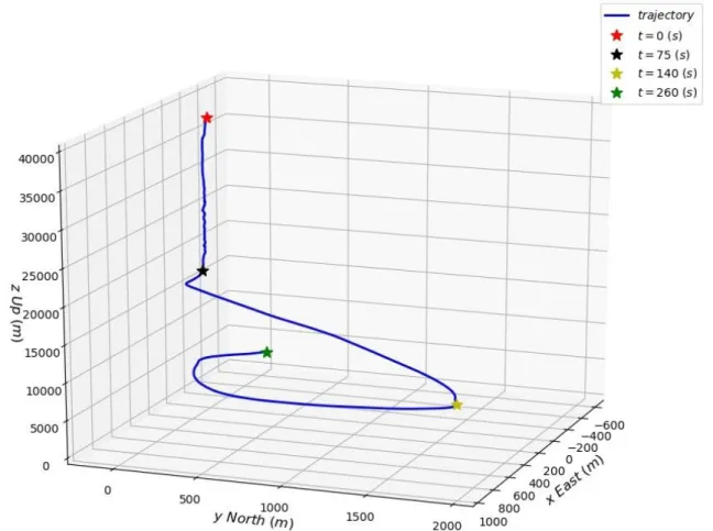
north 𝑦𝑁𝑜𝑟𝑡ℎ and the up 𝑧𝑈𝑝. In this local ENU (East, North, Up) coordinate system, the trajectory 98
versus time is depicted in figure 1. This representation has not been used by other authors who studied 99
the free fall, but it is very interesting, more intuitive and practical. In figure (1), we can clearly identify 100
two stages of the leap’s evolution. The first stage, from exit time t=0 to 75 s, is a quasi-perfect vertical 101
one dimensional movement. The second stage from t=75 to t=260 s (main chute deployment, at 102
18:10:52.0 UTC) looks more like a classic free fall of a skydiver who does not try to increase his speed 103
but instead tries to fall slowly and steadily in a nice regular “belly-to-earth” position. 104
In most papers [4,5 and 8], the acceleration due to gravity is taken as constant, but the change of g can 105
be easily considered by using the world geodetic system ellipsoidal gravity formula (WGS 1984) with 106
the first-order free-air correction factor: 107
𝑔(𝑧, 𝜑) = 9.7803 1+0.00193∙𝑠𝑖𝑛2(𝜑)
√1−0.00669∙𝑠𝑖𝑛2(𝜑)− 3.086 × 10
−6∙ 𝑧 (4)
108
at the origin of local ENU system 𝜑 = 33.3408417° 109
𝑔(𝑧, 𝜑) = 9.7959 − 3.086 × 10⁻⁶∙ 𝑧 (5) 110
For z varying from the initial position to the main chute deployment, 2566.8 ≤ 𝑧 ≤ 38969.4 m, the 111
acceleration due to gravity is 9.6756 ≤ 𝑔 ≤ 9.7879 𝑚 𝑠⁄ , that is a relative error of 1% if g is taken 2 112
as a constant. The total mass of Baumgartner taken for the simulations is 𝑚 = 121.2 𝑘𝑔 [7]. 113
For this experience, the Red Bull Stratos team did everything to ensure the safety of Baumgartner’s 114
jump [1; 10]. Various measures have been taken, analyzed and processed by the team to validate 115
several world records, and now they are available to us. Baumgartner was equipped with several GPS 116
apparatuses, and in particular a Garmin 18X-5 WAAS GPS with a sampling frequency of 5 position 117
measurements per second. The data files made available also contain temperature, air pressure, speed 118
of sound and triaxial acceleration data. Baumgartner was equipped with a triaxial accelerometer 119
positioned at chest level in order to understand and analyze the environmental stressors experienced 120
[11]. 121
Atmospheric density and speed of sound (𝑀𝑎𝑐ℎ1) profiles are estimated based on the pressure 𝑃(𝑧) 122
and temperature 𝑇(𝑧) measurements with: 123
𝜌(𝑧) = 𝑃(𝑧)
𝑅𝑠𝑇(𝑧) and 𝑀𝑎𝑐ℎ1(𝑧) = √1.40 ∙ 𝑅𝑠𝑇(𝑧) (6 and 7)
5 with 𝑅𝑠= 287.0 𝐽 (𝐾 𝑘𝑔)⁄ . The profiles of temperature, pressure, density and speed of sound are 125
depicted in figure 2 (red curve) and are compared to two classical models, the US Standard 126
atmosphere, 1976 [12] and NRLMSISE-00 Atmosphere Model [13, 14], and to the sounding operated 127
by the Red Bull Stratos team at the Santa Teresa observatory and Roswell airport. The most important 128
data for studying the free fall is for 20 ≤ 𝑧 ≤ 40 km. In this part, we have good correlation between 129
the data and the NRLMSISE-00 Atmosphere Model. In the later simulations we will use the data 130
depicted on the red curve. To our knowledge, the data was obtained by the Red Bull Stratos team with 131
a numerical weather forecast model. 132
For the drag coefficient and the projected area, we use the relations proposed by Guerster and 133 Walter [7]: 134 𝐶𝐷= 𝐴 for 𝑀𝑎 = 𝑣𝑧 𝑀𝑎𝑐ℎ1≤ 0.6 (8) 135 𝐶𝐷= 𝐴 + 𝐵(𝑀𝑎 − 0.6)2 for 0.6 ≤ 𝑀𝑎 ≤ 1.1 (9) 136 𝐶𝐷= 𝐴 + 0.25 ∙ 𝐵 − 𝐶(𝑀𝑎 − 1.1) for 1.1 ≤ 𝑀𝑎 (10) 137 and 138 𝐴⊥(𝛽) = 𝐴𝑥sin(𝛽) + 𝐴𝑧cos(𝛽) (11) 139
with 𝐴𝑥 = 1.19 𝑚2 the effective front area and 𝐴𝑧 = 0.525 𝑚2 the effective top area [7], A, B and C 140
three parameters that should be estimated in the inverse problem. 141
The last needed information, and probably the most difficult to obtain is the angle of attack 𝛽 during 142
the leap. Guerster and Walter [7], estimate an angle of attack 𝛼 =𝜋2− 𝛽 with the full video from 143
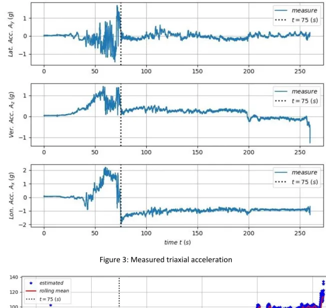
Baumgartner’s point of view during the leap. In this study, the angle of attack is estimated based on 144
the triaxial acceleration measurements (fig.3). Accelerometers are sensitive to both linear acceleration 145
and the local gravitational field. In the absence of linear acceleration, the accelerometer output is a 146
measurement of the rotated gravitational field vector and can be used to determine the accelerometer 147
orientation angles. At the start of a fall, the vector sum of acceleration will tend toward 0 g (fig 3) - 148
this is called the phenomenon of weightlessness. Until t=25 s, the longitudinal and lateral accelerations 149
do not change, after that time and until t=75 s, these accelerations fluctuate a lot. During this time, 150
Baumgartner was in a dangerous situation of spinning, which has been studied in detail by Garbino et 151
al. [11]. The vertical acceleration has a different signal: it changes gradually, probably due to the drag 152
force’s module and direction acting on the body (fig. 3). Even if we aren’t in a perfectly static situation, 153
and we also neglect the lateral acceleration 𝐴𝑦, and if we suppose likewise that Baumgartner didn't 154
rotate around his body’s z-axis (head first), the angle of attack is estimated with [15, eq. 55 page 19]: 155
𝛽 = 𝑐𝑜𝑠−1( 𝐴𝑧
√𝐴𝑥2+𝐴𝑧2
) (12) 156
6 with 𝐴𝑧 and 𝐴𝑥 representing the vertical and longitudinal acceleration respectively. In order to smooth 157
the signal and remove potential linear acceleration, a rolling mean of 2.5 s is applied to the angle and 158
used later in a linear interpolation lookup table for the simulations (fig. 4). 159
The numerical implementation
160
The programming language we use is Python, a language which gives readable code that closely 161
resembles the equations. The equation (3) is a system of two first-order equations that can be solved 162
by numerical integration. There are a lot of numerical tools called “ODE solver” (ordinary differential 163
equation) to solve this kind of equation [16]. Here, we have chosen to work with the SciPy ecosystem 164
[17], and in particular with the module scipy.integrate.solve_ivp. This module allows us to choose 165
between all the classical numerical integration methods, and trigger events to stop the integration 166
time if needed. By default, we select the Runge-Kutta method. We can also set the maximum allowed 167
time step size during integration, which allows us to properly control any variations in the parametric 168
functions, like the angle of attack. At this stage, we have all the necessary information allowing us to 169
program and to solve the direct problem, apart from the parameters A, B and C appearing in the drag 170
force. A useful solution is to generate uniformly distributed random parameters between bounds 171
and/or to take some values from literature and to build the code and do tests. This is an important 172
step before tackling the inverse problem, since the direct code must be solved in as little CPU time as 173
possible, and be reliable and robust regardless of the parameters used. 174
175
III. The inverse problem 176
The inverse problem covers a very wide range of formulations and fields of application. In this part, we 177
will present an application of a classical non-linear inverse problem. Here, the aim is to find the model 178
parameters we don't know that produce the data we have measured. From a mathematical point of 179
view, we formulate this with the help of a classical cost function or objective function, i.e. the mean 180
sum square error between model output and the measures: 181 𝑂(𝑝; 𝑦, 𝑦𝑚𝑒𝑠) = 1 𝑛𝑚−𝑛𝑝∑ (𝑦𝑖(𝑝) − 𝑦𝑖 ∗)2 𝑛𝑛 𝑖=1 (13) 182
with 𝑝 = (𝐴, 𝐵, 𝐶) the vector of parameters, nm and np the number of measurements and parameters 183
respectively, 𝑦𝑖(𝑝) the model output, e.g. the speed and 𝑦𝑖∗ the measurements. The aim is to find the 184
parameters that minimize the objective function, which is done iteratively. Generally, the algorithm 185
starts with a set of initial parameters and calculates the corrections to be made to the parameters, so 186
that the objective function decreases until a criterion of the objective function is reached and/or until 187
the parameter values don't change anymore. There are plenty of algorithms that can be used to 188
minimize a function. The most widely used is probably the Levenberg-Marquardt algorithm. The choice 189
of a good algorithm is problem dependent, on the number of parameters, the bounds on the 190
7 parameters, the number of available measurements, the correlations between parameters, the 191
structure of the model and so forth. We can distinguish two main classes of algorithms: global and 192
local algorithms. According to the author's own experience, the most efficient strategy when solving a 193
minimization problem is to be able to use several kind of algorithms and analyze the different results. 194
Here, we have chosen to use LMFIT: Non-Linear Least-Squares Minimization and Curve-Fitting for 195
Python [18]. This library allows us to use more than twenty methods of minimization, from the local 196
Levenberg-Marquardt least squares method to the Markov Chain Monte Carlo (MCMC) algorithm, 197
amongst others. A complete discussion of inverse methods is beyond the scope of this document; the 198
aim here is simply to give students access to up-to-date methods and algorithms as "gray-box", and 199
not completely "black-box". 200
The use of lmfit.minimize() module is straightforward, as long as the user starts with one of the 201
numerous examples available on the GitHub repository (
https://lmfit.github.io/lmfit-202
py/examples/index.html) and adapts it to their problem. Principally, the user has to build a callable 203
function that corresponds to the direct problem. This function should return the difference between 204
model and measure, i.e. the residual vector: 205
𝜀𝑖 = 𝑦𝑖(𝑝) − 𝑦𝑖∗ (14) 206
In our example, the state variable of interest is the speed. 𝑦𝑖(𝑝) is the solution of the system of 207
equation (3), i.e. 𝑣𝑧(𝑡 = 𝑡𝑖), with 𝑡𝑖 the discrete time observations for 𝑖 = 1 ⋯ 𝑛𝑚. In the local ENU 208
coordinate system, we can compute the speed by using the evolution of the altitude z over time with 209
a first order finite difference equation: 210
𝑦𝑖∗≡ 𝑣𝑖≃
𝑧𝑖+1(𝑡𝑖+1)−𝑧𝑖(𝑡𝑖)
𝑡𝑖+1−𝑡𝑖 (15) 211
The GPS used has a sampling frequency of 5 position measurements per second; for the whole duration 212
of the leap (from t=0 to 260s), this gives us a total number of available measurements of 1300. In figure 213
(1), we have seen that the vertical free fall is well approximated during only the first part of the leap, 214
that is for a period from t=0 to 75 s. For the parameter estimation, we only use the data obtained 215
during this first part of the leap and with one measurement per second, that is a total number of 216
measurements 𝑛𝑚 = 75, for a total number of parameters to be estimated 𝑛𝑝 = 3. 217
218
IV. Results and discussion 219
In order to start the inverse problem, it is often necessary to have some prior knowledge of the 220
parameters we want to estimate. Sometimes, these parameters have no physical meaning, but even 221
in this case we should give an initial set of parameters and some lower and upper bound values (Table 222
1). For this simulation, we use the trust region reflective method to minimize the objective function 223
8 [18]. At the end of the estimation, after 11 iterations, the final set of parameters and the 95% 224
confidence interval on the parameters are: 225 𝐴 = 0.617 +/− 0.035 (5.7%) (16) 226 𝐵 = 0.840 +/− 0.259 (30.8%) (17) 227 𝐶 = 1.425 +/− 0.344 (24.2%) (18) 228
The results differ from those of Guerster and Walter [7] for the parameters B and C. We find slightly 229
larger values for almost identical confidence intervals. It should be noted that the parameters A and B 230
have a correlation of -0.92 and for B and C of 0.89. Since we didn't use exactly the same angle of attack 231
as Guerster and Walter [7], it is possible to find different parameters that give almost identical results 232
for the speed. This is a key point for parameter estimation, as there is not always a unique solution to 233
the inverse problem, but instead depends greatly on the model structure and on available data. The 234
drag force in the model depends on the product of the drag coefficient and the projected area, so this 235
creates a perfect correlation between them. Colino and Barbero’s [6] strategy was to use the product 236
and take different values of this product depending on the stages of the leap. The results of the inverse 237
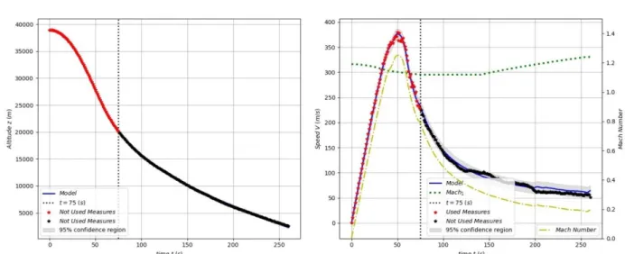
problem for the altitude, speed and Mach number are depicted in figure (5). We can observe a fairly 238
good match between the measurements and the modelling. The gray region (fig. 5) represents the 95% 239
confidence interval of the estimated speed. In the second stage, from t=75 to t=260 s, we observe 240
larger differences between the measurements and the model, probably due to a 3D effect on the 241
trajectory. A more detailed graphic concerning the supersonic stage is given in figure (6). We found a 242
total supersonic time of 30s, a maximum speed, reached at t=50 s, 𝑣 = 375.7 ± 10.8 𝑚 𝑠⁄ and a 243
Mach number 𝑀𝑎 = 1.25 ± 0.03. We can also see the impact of variations over time of the angle of 244
attack on the speed, for t=40 s and t=74 s. 245
Now that the whole model has been built (direct and inverse), it is relatively simple to carry out 246
additional tests if needed, for example to test other sets of initial parameters, or to assume that g is 247
constant, or to propose a different model for the drag coefficient or for the air density equation, or to 248
modify the time parametric function for the angle of attack. 249
If one wishes to have more reliable information on the parameters and their uncertainties, it is possible 250
with LMFIT to use an MCMC algorithm to determine the posterior distributions for the parameters, 251
and not only a local uncertainty estimation. 252
253
V. Conclusion 254
The good thing about building a full model, i.e. direct and inverse, is that it gives students the 255
opportunity to learn multiple skills by discussing the problem on the conceptual level, together with 256
mathematical formulation, finding numerical methods, appropriate algorithms and writing the 257
computer code, and testing the programs and using them to perform numerical experiments, to 258
9 analyze the problem, and to compare the results to real data. All of this is now possible, especially with 259
Python if we agree to use some libraries as a "gray-box" and explain the principles of these algorithms 260
to students. Additionally, representing the computational results graphically is always very important, 261
and this is facilitated for students with Python [19]. Finally, teaching the building of an inverse problem 262
has a lot of similarities with creating an Investigative Science Learning Environment [20, figure 1.3 page 263 1-7 ]. 264 265 Acknowledgments 266
A special thanks to Jonathan Clark and Alex Garbino, Department of Medicine, Section of Emergency 267
Medicine and Center for Space Medicine, Baylor College of Medicine, Houston - TX, for support and 268
making the flight data available to us. A sincere thank you to our colleague, Rob Simmons, from Institut 269
Universitaire de Technologie Louis Pasteur, for his diligent proofreading of the article. 270
271
References: 272
[1] Red Bull Stratos www.redbullstratos.com. 273
274
[2] Red Bull Stratos: Full Scientific Data Report, Findings of the Red Bull Stratos Scientific Summit, 275
California Science Center, Los Angeles, California, USA January 23, 2013, 276
https://issuu.com/redbullstratos/docs/red_bull_stratos_summit_report_final_050213.
277 278
[3] Samsonau S. V.,2018. Computer simulations combined with experiments for a calculus-based 279
physics laboratory course, Phys. Educ. 53 055013. 280
281
[4] Benacka J., 2010. High-altitude free fall revised. American Journal of Physics 78(6)616-619; doi: 282
10.1119/1.3298375. 283
284
[5] Theilmann F. and Apolin M., 2013. Supersonic freefall—a modern adventure as a topic for the 285
physics class. Phys. Educ. 48(2)150-158. 286
287
[6] Colino J. M. and Barbero A. J., 2013. Quantitative model of record stratospheric freefall. Eur. J. Phys. 288
(34)841–848, doi:10.1088/0143-0807/34/4/841. 289
290
[7] Guerster M. and Walter U., 2017. Aerodynamics of a highly irregular body at transonic speeds— 291
Analysis of STRATOS flight data. PLoS ONE 12(12): e0187798; doi: 10.1371/journal.pone.0187798. 292
10 [8] Corvo T., 2019. An Analytical Solution to the Extreme Skydiver Problem. The Physics Teacher 294
57:287-289; doi: 10.1119/1.5098912. 295
296
[9] Barger V. and Olsson M., 1995. Classical Mechanics: A Modern Perspective, Second Edition, 297
McGraw-Hill, New York, 418pp. 298
299
[10] Blue R.S., Law J., Norton S.C., Garbino A., Pattarini J. M., Turney M. W., Clark J.B., 2013. Overview 300
of medical operations for a manned stratospheric balloon flight. Aviat Space Environ Med (84)237-41. 301
302
[11] Garbino A., Blue R.S., Pattarini J. M., Law J., Clark J.B., 2014. Physiological monitoring and analysis 303
of a manned stratospheric balloon test program. Aviat Space Environ Med (85)177–82. 304
305
[12] U.S. standard atmosphere, 1976, Washington, D.C., NOAA--S/T 76-1562,241pp. 306
307
[13] J.M. Picone, A.E. Hedin, D.P. Drob, and A.C. Aikin, 2002. NRLMSISE-00 empirical model of the 308
atmosphere: Statistical comparisons and scientific issues, J. Geophys. Res., 107(A12), 1468, 309
doi:10.1029/2002JA009430. 310
311
[14] Papitashvili N. 2001. Web interface for NRLMSISE-00 Atmosphere Model, The Community 312
Coordinated Modeling Center, https://ccmc.gsfc.nasa.gov/modelweb/models/nrlmsise00.php. 313
314
[15] Pedley M., 2013. Tilt Sensing Using a Three-Axis Accelerometer. Freescale Semiconductor, Inc. 315
AN3461 Application Note Rev. 6, 22pp. 316
317
[16] Linge S. and Langtangen H. S., 2020. Programming for Computations – Python : A Gentle 318
Introduction to Numerical Simulations with Python 3.6, Second Edition, Springer Open, 350pp. 319
https://doi.org/10.1007/978-3-030-16877-3. 320
321
[17] Pauli Virtanen, Ralf Gommers, Travis E. Oliphant, Matt Haberland, Tyler Reddy, David Cournapeau, 322
Evgeni Burovski, Pearu Peterson, Warren Weckesser, Jonathan Bright, Stéfan J. van der Walt, Matthew 323
Brett, Joshua Wilson, K. Jarrod Millman, Nikolay Mayorov, Andrew R. J. Nelson, Eric Jones, Robert Kern, 324
Eric Larson, CJ Carey, İlhan Polat, Yu Feng, Eric W. Moore, Jake VanderPlas, Denis Laxalde, Josef 325
Perktold, Robert Cimrman, Ian Henriksen, E.A. Quintero, Charles R Harris, Anne M. Archibald, Antônio 326
H. Ribeiro, Fabian Pedregosa, Paul van Mulbregt, and SciPy 1.0 Contributors. (2020) SciPy 1.0: 327
11 Fundamental Algorithms for Scientific Computing in Python. Nature Methods,
328
https://doi.org/10.1038/s41592-019-0686-2. 329
330
[18] Newville M., Stensitzki T., Allen D. B. and Ingargiola A., 2014. LMFIT: Non-Linear Least-Square 331
Minimization and Curve-Fitting for Python (Version 1.0.1). Zenodo. 332
http://doi.org/10.5281/zenodo.11813. 333
334
[19] Weber J. and Wilhelm Th., 2020. The benefit of computational modelling in physics teaching: a 335
historical overview, Eur. J. Phys.41 034003. 336
337
[20] Etkina E., Brookes, D. T. and Planinsic G., 2019. Investigative Science Learning Environment. When 338
learning physics mirrors doing physics. Morgan & Claypool Publishers, 138pp. 339
http://dx.doi.org/10.1088/2053-2571/ab3ebd. 340
12 342
Figure 1: Skydiver position evolution through the leap, expressed in a local tangent plane coordinates 343
system, as origin (𝜑 = 33.3408417°, 𝜆 = −103.7679067°, 𝑧 = 0.0 m) 344
345
346
Figure 2: Comparison of the different atmospheric data; the red curves are used for the simulations. 347
13 348
Figure 3: Measured triaxial acceleration 349
350
Figure 4: Estimated angle of attack based on the acceleration 𝐴𝑥 and 𝐴𝑧 351
14 Table 1: Initial set of parameters with lower and upper bounds.
353
Parameters 𝑝𝑘 Min value Initial value Max value
A 0.25 0.6 2 B 0.1 0.6 2 C 0 0.3 5 354 355 356
Figure 5: Measured and predicted altitude, speed and Mach number with the final set of parameters. 357
358
Figure 6: Measured and predicted altitude, speed and Mach number with the final set of parameters 359
for the supersonic stage. 360