The Cluster Magnetic Field Investigation: overview of in-flight performance and initial results

HAL Id: hal-00316910

https://hal.archives-ouvertes.fr/hal-00316910

Submitted on 1 Jan 2001

HAL is a multi-disciplinary open access

archive for the deposit and dissemination of

sci-entific research documents, whether they are

pub-lished or not. The documents may come from

teaching and research institutions in France or

abroad, or from public or private research centers.

L’archive ouverte pluridisciplinaire HAL, est

destinée au dépôt et à la diffusion de documents

scientifiques de niveau recherche, publiés ou non,

émanant des établissements d’enseignement et de

recherche français ou étrangers, des laboratoires

publics ou privés.

in-flight performance and initial results

A. Balogh, Chris M. Carr, M. H. Acuña, M. W. Dunlop, T. J. Beek, P.

Brown, K.-H. Fornacon, E. Georgescu, Karl-Heinz Glassmeier, J. Harris, et al.

To cite this version:

A. Balogh, Chris M. Carr, M. H. Acuña, M. W. Dunlop, T. J. Beek, et al.. The Cluster Magnetic Field

Investigation: overview of in-flight performance and initial results. Annales Geophysicae, European

Geosciences Union, 2001, 19 (10/12), pp.1207-1217. �hal-00316910�

Geophysicae

The Cluster Magnetic Field Investigation: overview of in-flight

performance and initial results

A. Balogh1, C. M. Carr1, M. H. Acu ˜na2, M. W. Dunlop1, T. J. Beek1, P. Brown1, K.-H. Fornacon3, E. Georgescu4, K.-H. Glassmeier3, J. Harris1, G. Musmann3, T. Oddy1, and K. Schwingenschuh5

1_{Imperial College, London, UK}

2_{NASA/GSFC, Greenbelt, Md., USA}

3_{IGM, TU Braunschweig, Germany}

4_{MPE, Garching, Germany}

5_{IfW, Graz, Austria}

Received: 21 March 2001 – Revised: 18 June 2001 – Accepted: 19 June 2001

Abstract. The accurate measurement of the magnetic field

along the orbits of the four Cluster spacecraft is a primary objective of the mission. The magnetic field is a key con-stituent of the plasma in and around the magnetosphere, and it plays an active role in all physical processes that define the structure and dynamics of magnetospheric phenomena on all scales. With the four-point measurements on Clus-ter, it has become possible to study the three-dimensional as-pects of space plasma phenomena on scales commeasurable with the size of the spacecraft constellation, and to distin-guish temporal and spatial dependences of small-scale pro-cesses. We present an overview of the instrumentation used to measure the magnetic field on the four Cluster spacecraft and an overview the performance of the operational modes used in flight. We also report on the results of the prelimi-nary in-orbit calibration of the magnetometers; these results show that all components of the magnetic field are measured with an accuracy approaching 0.1 nT. Further data analysis is expected to bring an even more accurate determination of the calibration parameters. Several examples of the capa-bilities of the investigation are presented from the commis-sioning phase of the mission, and from the different regions visited by the spacecraft to date: the tail current sheet, the dusk side magnetopause and magnetosheath, the bow shock and the cusp. We also describe the data processing flow and the implementation of data distribution to other Cluster in-vestigations and to the scientific community in general.

Key words. Interplanetary physics (instruments and

tech-niques) – magnetospheric physics (magnetospheric configu-ration and dynamics) – space plasma physics (shock waves)

1 Introduction: scientific objectives of the Cluster Mag-netic Field Investigation

Magnetic fields are a key component of space plasmas. They provide the basic physical reference system for the transport

Correspondence to: A. Balogh (a.balogh@ic.ac.uk)

of momentum and energy in the plasma. Boundaries be-tween plasmas of different origin, which often consist of thin current sheets, are recognised primarily through their signa-tures in magnetic field observations. Wave phenomena in the plasma are also ordered with respect to the underlying magnetic field. The Cluster mission brings a further, unex-plored dimension to magnetic field observations: using the measurement of the magnetic field vector at four points, a range of new parameters, such as the current density vector, the propagation vectors of waves, as well as the orientation, non-planarity, and motion of boundary surfaces can be de-termined. Additionally, the four-point magnetic field mea-surements are needed for the determination of the internal structure of the boundary regions. Such measurements are also essential for describing the parameters of turbulence in the different plasma regimes in and around the Earth’s mag-netosphere. Magnetic field vector measurements at the four Cluster spacecraft provide, therefore, an essential ingredient for meeting the scientific objectives of the mission.

The primary objective of the Cluster Magnetic Field In-vestigation (FGM) is to provide accurate measurements of the magnetic field vector at the location of the four Cluster spacecraft. The many scientific objectives that are related to the physics of space plasmas in the Earth’s magnetosphere and in its vicinity all use the basic measurements of the mag-netic field vector. We enumerate here a brief summary of the detailed objectives presented previously (Balogh et al., 1993, 1997).

The Cluster orbit samples most of the key regions of the magnetosphere. In the dayside boundary of the magneto-sphere, both at mid-latitudes and in the cusp, processes as-sociated with magnetic reconnection and turbulence are be-lieved to occur which control the dynamics of the solar wind interaction with the Earth’s magnetic field (e.g. Paschmann, 1995; Scholer, 1995). On the nightside, in the near-Earth magnetospheric tail, frequent large-scale magnetic reconfig-urations occur during substorms in which the tail plasma and current sheets plays a key role. On the flanks and on the dayside of the magnetosphere, there is a wealth of plasma

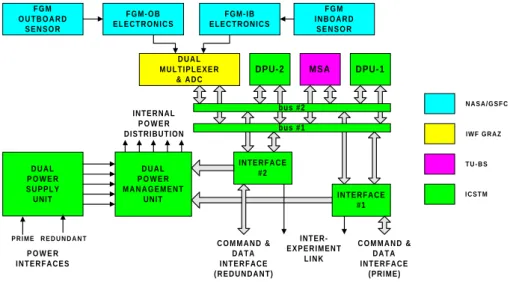
F G M O U T B O A R D S E N S O R F G M I N B O A R D S E N S O R D U A L M U L T I P L E X E R & A D C F G M - O B E L E C T R O N I C S FGM-IB E L E C T R O N I C S bus #2 bus #1 DPU-1 DPU-2 MSA INTERFACE #1 INTERFACE #2 D U A L P O W E R S U P P L Y UNIT D U A L P O W E R M A N A G E M E N T UNIT INTERNAL P O W E R DISTRIBUTION C O M M A N D & DATA INTERFACE ( R E D U N D A N T ) INTER-E X P INTER-E R I M INTER-E N T LINK P O W E R INTERFACES R E D U N D A N T P R I M E C O M M A N D & DATA INTERFACE (PRIME) N A S A / G S F C IWF GRAZ T U - B S I C S T M

Fig. 1. Block diagram of the FGM instrument on Cluster.

phenomena on many scales at the bow shock and in the mag-netosheath (for a first four-point study of mirror structures in the magnetosheath, see Lucek et al., 2001). The anisotropy which is inherent in all magnetised plasma processes, intro-duced by the magnetic field, makes the accurate determina-tion of the magnetic field at high time resoludetermina-tion a critical contribution to the probing of small-scale structures and dy-namics encountered in these regions (Southwood, 1990).

The current understanding of the structure and dynamics of the main boundaries on the sunward side of the magne-tosphere, the bow shock and the magnetopause is based, to a large extent, on observations of single crossings and nu-merical simulations. Some two-point observations are avail-able that have identified some of the temporal and spatial variability at these boundaries and in the upstream medium (Thomsen, 1988; Elphic, 1988 and Russell, 1988). How-ever, these boundaries have complex, evolving structures and are non-stationary on several time- and length scales. Four-point magnetic field observations provide information on the immediate neighbourhood of the boundaries that clarify the phenomenology of boundary-associated phenomena simul-taneously at the four locations. Magnetopause structure is clearly a complex topic, with relevance to a wide range of phenomena that contribute (and are affected by) the detailed processes that occur at this boundary. The first magnetic field investigation of the magnetopause by Cluster has been pre-sented by Dunlop et al. (2001a); a joint investigation of the magnetopause using low frequency wave and magnetic field data has been carried out by Rezeau et al. (2001).

A particularly interesting objective of Cluster on this topic is the exploration of processes occuring at quasi-parallel bow shock geometries, where the generally accepted shock re-formation occurs (Scholer and Burgess, 1992). Boundary crossing phenomena include complex wave fields that are an integral part of the MHD processes that form the wider en-vironment of the boundaries; inherent non-stationarity pre-vents the resolution of these wave fields by single- or even

two-point measurements. During a two-year mission, Clus-ter will cross the dayside bow shock and magnetopause sev-eral hundred times. This will allow the observation of both boundaries under a range of conditions that provide the basis for a separation of different phenomena and causal processes, as outlined in numerical simulations before the mission (e.g. Giacalone et al., 1994). The magnetometers on Cluster have already shown that they can generate the necessary data sets to determine the context and processes at these boundaries (see Sect. 6 and Horbury et al., 2001).

Other specific phenomena for four-point analysis to which the observations of the magnetic field on Cluster will con-tribute include dayside magnetic reconnection and the nature of flux transfer events in particular; the role of the Kelvin-Helmholtz instability in magnetopause processes; impulsive events, possibly driven by discontinuities in the solar wind; and, as a prime objective of Cluster, the nature, structure and dynamics of the outer cusp. For a first exploration of the capabilities of the Cluster magnetic field observations in the cusp, see Cargill et al. (2001).

In the magnetospheric tail, Cluster observations will target both phenomena at small-scales, such as the structure and time evolution of current sheets associated with the growth phase of substorms and, on larger scales, to establish the magnetic topology of the different regions in the tail and their dynamics. The role, in particular, of a range of current struc-tures and their magnetic signastruc-tures, all on scales which re-quire high time resolution magnetic measurements, simulta-neously at several locations, will contribute to resolving the time evolution of the magnetospheric tail prior to and during substorms.

A significant subset of the objectives of the magnetic field investigation has close connections with the wider field of solar-terrestrial relations. In this context, collaboration with simultaneous ground-based observations is already playing a key role in relating magnetospheric responses with signa-tures observed by remote-sensing, ground-based instruments

Table 1. Operative ranges for the FGM (not all used)

Range No. Range Resolution

2 −64 nT to +63.97 nT 7.8×10−3nT 3 −256 nT to +255.87 nT 3.1×10−2nT 4 −1024 nT to +1023.5 nT 0.125 nT 5 −4096 nT to +4094 nT 0.5 nT 7 −65536 nT to +65504 nT 8 nT

and facilities, such as magnetometer chains and ionospheric radars (Wild et al., 2001).

The analysis of four-point magnetic field measurements presents formidable conceptual and technical challenges. The techniques developed for Cluster have a rich literature; an important review of the multipoint analysis techniques was published by a Working Group of the International Space Science Institute (Paschmann and Daly, 1998, chapters and references therein). The Cluster magnetometer team also published several aspects of four-point analysis techniques specifically related to magnetic field data since 1990 (for a comprehensive list of publications on this topic, see Balogh and Dunlop, 2000, but also Dunlop et al., 1996, 1997; Dun-lop and Woodward, 1998, 2000). First reviews of applica-tions of these techniques using Cluster magnetic field data are presented in Dunlop et al. (2001b), and Glassmeier et al. (2001).

2 Overview of the FGM instrument

The FGM instrument on each spacecraft consists of two tri-axial fluxgate magnetic field sensors on one of the two radial booms of the spacecraft, and an electronics unit on the main equipment platform. The block diagram of the instrument is shown in Fig. 1. The instrument is designed to be highly failure-tolerant through a full redundancy of all its functions. In particular, either of the two magnetometer sensors can be used as the primary sensor for the main data stream from the instrument, although in normal operations, the outboard sen-sor, located at the end of the 5 m radial boom, is designated as the primary source of the data. The magnetometers can measure the three components of the field in seven ranges, although only four of these (numbered 2 to 5) are used on Cluster, with full scales and the corresponding digital resolu-tions as shown in Table 1. Another range (range 7) was used only for ground testing.

Switching between ranges is either automatic, controlled by the instrument Data Processing Unit (DPU) in flight, or set by ground command. When in the automatic mode, a range selection algorithm running in the DPU continuously monitors each component of the measured field vector. If any component exceeds a fraction (set at 90%) of the range, an up-range command is generated and transmitted to the sensor at the start of a new telemetry format. (All three components are measured in the same range.) If all three components are

0.0

44.6

89.2 133.8 178.4 223.0

Time (ms)

0.0

74.4

148.7

223.0

22.417 vectors/s

67.25 vectors/s

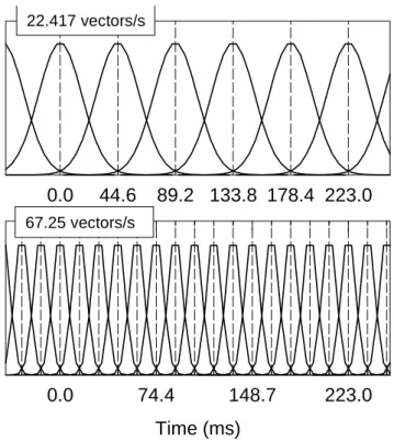
Fig. 2. Gaussian digital filtering of the full resolution sampling at

201.75 vectors/s of the magnetic field. The two most frequently used vector sampling rates are illustrated.

smaller than 12.5% of the range for more than a complete spin period, a down-range command is implemented at the start of the next vector. The facility to override the automatic ranging is included partly for test purposes, and partly as a capability for failure recovery.

3 Overview of the FGM instrument

The sampling of vectors from the magnetometer sensor des-ignated as the primary sensor is carried out at the rate of 201.793 vectors/s. This internal sampling rate has been se-lected to provide an appropriate set of lower rates (after filter-ing) for the different telemetry modes and to give the highest frequency response for the short periods of interest recorded in the MSA. In order to ensure the high stability of the

sam-pling rate, the clock signal used for it is derived from a 223Hz

crystal oscillator internal to the instrument. The primary re-quirement is that the sampling of vectors be carried out at equal time intervals. This requirement is implemented by sequencing the software by the sampling clock and by en-suring that all software sequences have a deterministic du-ration. The full bandwidth of the sampled vectors cannot be routinely transmitted via the telemetry due to the lim-ited telemetry rate allocation. The Central Processor Unit encompasses the full bandwidth of data with a Gaussian dig-ital filter to match the rate and bandwidth of the transmitted vectors to the available telemetry rate. The filter coefficients are selected from stored sets corresponding to the different

HF Clock counter reading = n

HF Clock counter reading = m output queue

subsequent filtered vectors at equal intervals

block and buffer vectors in output queue v e c t o r s s a m p l e d

at 201.75 Hz Gaussian digital filter filtered vectors for telemetry transmission

start time of filter of first

vector first vector of telemetry format

resets marking start/end of telemetry format p a c k e t h e a d e r FGM auxiliary data F G M vector data 5 . 1 5 2 2 2 2 s e c o n d s U T C F G M s c i e n c e p a c k e t

Fig. 3. Internal generation of the timing data for transmission though the spacecraft telemetry to ensure the accurate reconstruction of the

vector timing by the ground processing.

telemetry modes. Filtering in the two most frequently used instrument modes is illustrated in Fig. 2.

Following the filtering, completed vector samples are stored in an output queue for the duration of a telemetry frame between reset periods. The recovery of the times at which the vectors were sampled is a very important require-ment. The timing chain which enables the conversion (after data recovery on the ground) is indicated schematically in Fig. 3. While timing of the samples is strictly based on the internal FGM clock, by recording and transmitting a time marker, based on the spacecraft provided HF clock, which corresponds to the first vector sample in a given telemetry frame, together with the reading of the same clock at the time of the start of the next telemetry frame, the vector sample se-quence can be unambiguously recovered.

4 Operational modes of the instrument

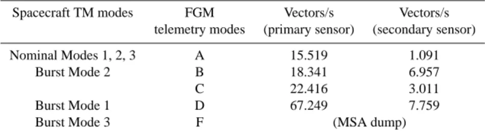
The operational modes of the instrument are matched to the different scientific telemetry modes of the spacecraft that de-fine the data rates available to the FGM. Additional param-eters of the operational modes are the proportions of data from the primary and secondary sensors, as well as whether data are read out from the Microstructure Analyser memory. The main operational modes of the FGM instrument are sum-marised in Table 2, together with the associated vector trans-mission rates through the telemetry.

A particular operation mode implemented late in the Clus-ter 1 programme and not described before allows one to over-come the limited sampling along the Cluster orbit. It is clear from the Cluster Master Science Plan that there are signifi-cant periods when there is no telemetry acquisition, with to-tal data coverage at approximately 50%. It is possible for the FGM instrument to take data during these data gaps and store it within the instrument for later transmission to Earth. To significantly extend the data coverage period, it is

neces-sary to reduce the data storage rate to less than that of the normally available FGM modes. A convenient rate is spin synchronised with one averaged vector per spin being stored to memory. In this way, an additional 27 h of data can be recovered from periods when there is no telemetry coverage. This is the FGM Extended Mode (FGMEXT).

Each FGM contains 192 Kbytes (96 K words) of memory, the Micro Structure Analyzer (MSA) which is normally used for capturing short periods of high resolution data. At the beginning of LOS (Loss of Signal), the FGM is commanded into FGMEXT which uses the MSA to store long periods of spin averaged data. Naturally, this data must be read out as soon as telemetry is restored so that the memory can revert to its normal purpose. This is achieved through the use of the BM3 dump (FGMOPM8) which normally occurs soon after the next acquisition of signal (AOS). FGMEXT was tested during the early phase commissioning of the FGM but did not become fully operational until after the BM3 dumps at AOS were routinely implemented in the Master Science Plan; thus, FGMEXT became operational on orbit 113 in February 2001. Data are taken only by the primary sensor (the out-board sensor by default); the primary sensor remains in the autoranging mode.

In this mode, the instrument synchronises acquisitions to spin sectors by measuring the Sun Reset Pulse (SRP) period and dividing by 512. These are then despun, averaged and stored to the MSA. Data timing is by the HF clock (4096 Hz) at points derived from a measure of the spin period. For ex-ample, with a 4 s spin period, each data point will be 32 ticks separated from its neighbours on either side. Data acquisi-tion is performed by calls to the routine normally used to read the secondary vectors and housekeeping voltages. Vec-tors are acquired with a delay of no more than 100 µs after the allotted clock transition.

Despinning is achieved in a similar way to that of the Ulysses instrument, i.e. by implementing Walsh transforms with Haar coefficients, where the Haar coefficients are given

Table 2. Magnetic vectors telemetered to ground for the operating modes of FGM

Spacecraft TM modes FGM Vectors/s Vectors/s telemetry modes (primary sensor) (secondary sensor)

Nominal Modes 1, 2, 3 A 15.519 1.091

Burst Mode 2 B 18.341 6.957

C 22.416 3.011

Burst Mode 1 D 67.249 7.759

Burst Mode 3 F (MSA dump)

by the equations in Table 3.

The Haar functions are simply +1 where the correspond-ing trigonometric function is positive and −1 where the cor-responding function is negative. They are undefined at the zero crossing points of the functions. As the number of points per spin is a power of 4, this means that data points are taken where the functions are undefined. For this rea-son the Haar functions are given a phase delay so that the transition lies between vectors. This is achieved onboard by establishing what quadrant a particular vector is being calcu-lated in and stating explicitly what the Haar coefficients are for all vectors in that quadrant, i.e. the coefficients are not calculated for each new angle.

The despun components are calculated from the spinning measurements, as shown in the equations in Table 3. Each vector is the arithmetic mean of 512 despun vectors over a single spacecraft spin. The data is susceptible to aliasing as the acquisition frequency is not greater than twice the cut off frequency of the onboard analogue filter, set to 90 Hz. Fur-thermore, the digital filter is a top hat which has associated side lobes in the frequency domain. Assuming that the spin period is 4 s and the code acquires a vector on the required HF clock tick (frequency = 4096 Hz, then each component

will be consistent with a resolution of 0.022◦.

Data sampled in FGMEXT is also written to the OnBoard Data Handling System (OBDH). Although there is no scien-tific telemetry, there is continuous housekeeping monitoring. For this reason, the FGM provides a reduced set of safety critical housekeeping parameters (power supply temperature, voltages, and reset count) for the purposes of onboard moni-toring.

Once the FGM is switched into FGMEXT, it remains in this mode until the instrument has filled up the MSA (23 h initially but this may be ramped up to 28 h depending on in-flight performance) or is switched back to FGMOPM1 due to AOS occurring. In both cases, the contents of the MSA are automatically frozen until transmission to Earth has been completed. It is possible to download the MSA contents in other telemetry modes (e.g. FGMOPM3) but the BM3 option is the most efficient. The housekeeping packet will provide an input into the Data Processing Software module that deals with FGMEXT, together with the contents of the MSA dump in order that the vector timeline can be accurately recovered. The µ/4 term is also included at this stage.

5 In-flight calibration: techniques and preliminary re-sults

The calibration of the magnetic field data is of key impor-tance for meeting the scientific objectives not only of the magnetic field investigation, but also those of the mission as a whole, as the interpretation of observations in terms of physical processes relies on the detailed comparison of mea-surements made at the four spacecraft. Calibration in this context represents the determination of parameters that al-low for the transformation of raw measurements transmitted through the telemetry into a magnetic field vector, given in physical units (nT), in an instrument-specific coordinate sys-tem that is unambiguously related to the coordinate syssys-tem of the spacecraft. The calibration parameters are used by the data processing software (see Sect. 5) to generate the magne-tometer data in a range of geophysical coordinate systems.

The in-flight calibration of FGM is based on an evaluation of all the possible sources of errors that occur in the measure-ment process, embodied in an “instrumeasure-ment model” represent-ing the measurement process of the magnetic field.

Concep-tually, given the actual value BGSEof the ambient magnetic

field vector at the location of the FGM sensor (given, for in-stance, in Geocentric Solar-Ecliptic, GSE, coordinates), the FGM output through the telemetry is a digitised vector V . This vector (the actual measurement) depends on in a com-plex way the alignment and orthogonality of the sensor axes with respect to the GSE coordinate system. This depends on the scale factors and offsets of the sensors and electronics of FGM and on the offsets introduced by the spacecraft. The in-strument model also needs to take into account the time and frequency response in the form of delays and effective band-width due to the magnetometers, the Analogue-to-Digital Converters, and the digital filtering process. The coordinate transformation from GSE into the (nearly, but not quite or-thogonal) magnetometer sensor system (specific to each of the eight magnetometers on the four Cluster spacecraft) is a complex superposition of transformations that also takes into account the misalignements introduced by the space-craft, the magnetometer booms, sensor mounting and con-struction. All these effects need, in principle, to be evaluated for each of the measured output vectors.

Ground calibration of the FGM instruments has allowed for the development of a practical model of the instruments, identifying the effective transformations that lead from the

Table 3. HAAR function definition for the extended mode use of

the MSA

CH(t) =_|Cos(ωt)|Cos(ωt) SH(t) =_|Sin(ωt)|Sin(ωt)

BY = PN−1 i=0 π 4[−BZSiSH i+BY SiCH i] N BZ= PN−1 i=0 π 4[BZSiCH i+BY SiSH i] N

BZ= Despun Z component BZS= Sampled Z component

B_Y= Despun Y component B_{Y S}= Sampled Y component

N= Number of points per spin = 512 CH, SH= Haar functions

ambient field to the measured output in the following form: V = c(instr)c(SR−FSR)c(spin)c(att)BGSE+c0.

The sensor matrix c(sensor)_=c(instr)_c(SR−FSR)_{represents the}

sensitivities (scale factors) of the sensors and the alignment of the three sensor axes with respect to an orthogonal coor-dinate system aligned with the real spin axis. The spacecraft

spin is taken into account in the rotation matrix c(spin),

corre-sponding to the spin-phase angle of sensors at the time of the

measurement. The matrix c(att)represents the transformation

into the spacecraft spin-aligned coordinate system from the GSE system. This matrix is determined from the spacecraft

attitude measurements. Finally, the vector c0represents the

offsets associated with the sensors and the spacecraft back-ground field at the location of the sensors.

The equation defining the measurements can be trans-formed to state the in-flight calibration task, i.e. to determine the relevant term in the inverted form of this equation: BGSE=c(att)

−1

c(spin)−1c(SR−FSR)−1c(instr)1(V − c0).

In the following, the steps performed by the first modules of the data processing software are described that implement the practical definition of the calibration parameters that need to be derived from the data. The digital output of the magne-tometer is a vector V in binary units. As a preparatory step, this vector is transformed into physical units, using a

diago-nal matrix of nomidiago-nal scale factors MST (nT/binary count),

to a vector BF Scorresponding to the tri-axial magnetometer

output in magnetic field units (uncalibrated, or “raw” nT): B_{F S}=M(ST )V

The coordinate system used in this equation is the FGM sen-sor system, defined by the true (magnetic) directions of the sensor triad; it is not exactly orthogonal, due to small inaccu-racies in the magnetic and mechanical alignment of the

sen-sors. The vector BF Sis used as an input to the next

process-ing step which then uses the calibration parameters to yield the magnetic field vector in physical units. In a coordinate system, this is denoted by FSR, which is the FGM spin refer-ence system, an orthogonal, right-handed coordinate system with its X-axis along the real spin axis of the spacecraft, and the Y -axis aligned with the sensor along the magnetometer boom. The defining equation of this transformation is BFSR=c(cal)BF S−ocal. Time (s) 0 2 4 6 8 10 12 14 Raw co unts -4000 -2000 0 2000 4000 6000 x y z CAL ON

Fig. 4. Implementation of the in-flight calibration mode of the FGM

instrument. The data illustrated are from an actual calibration se-quence on spacecraft 1. When the calibration mode is switched on, a train of square wave, consisting of 512 on-off applications of a fixed value calibration signal is internally superposed on the ambi-ent field measured by the instrumambi-ent. The frequency of the square wave is matched to the filtering bandwidth of the vector sampling.

The objective of the in-flight calibration is to determine the

3 × 3 matrix c(cal) and the offset vector ocal used in this

equation for all magnetometers on the four spacecraft, for all ranges and, in each case, for both A–D converters. The

calibration matrix c(cal)depends on a number of effects that

include range-dependent scale factors, deviations of the sen-sor axes from orthogonality, scale factor deviations between the two A–D converters and the alignment of the sensor axes

to the spin axis system. The offset vector ocal depends on

both spacecraft-induced and sensor offsets. Despinning, i.e.

the application of the matrix c(spin)−1, as well as the

coor-dinate transformation c(att)−1 into a physical coordinate

sys-tem, such as GSE, are performed, as outlined below, in the routine data processing of the FGM data. The built-in in-flight calibration mode (FGMCAL) is initiated nominally once per orbit, or at a slower rate, as considered appropri-ate, given that its application involves the disabling of the FGM data on Inter-Experiment Link, preventing other inves-tigator from receiving the data used for their onboard pro-cessing. This mode provides information on the sensitivity factors and alignment of the three axes of the FGM primary sensor. In this mode, an internally generated calibration sig-nal is applied to the primary sensor, following a preset se-quence. The full sequence consists of 512 cycles of CAL ON and CAL OFF steps, with a 50% duty cycle. The fre-quency of the steps is one half of the Nyquist frefre-quency of the current primary science output. For instance, in the nom-inal mode (FGM Op Mode 1), at 22.4217 vectors/s trans-mission rate, the frequency of the on-off calibration signal is 22.4217/4 = 5.60 Hz. The operation of the in-flight cal-ibration mode is illustrated in Fig. 4. The raw telemetry output of the instrument is illustrated, prior to despinning, calibration and transformation into physical units and

phys--80 -60 -40 -20 0 R e la ti ve sig nal st re ngt h (db) -80 -60 -40 -20 0 Frequency (Hz) 0 2 4 6 8 10 -80 -60 -40 -20 0 X-component Y-component Z-component spin 5.60 Hz

Fig. 5. Frequency domain analysis of the in-flight calibration

se-quence shown in Fig. 4 for the three components of the magnetic field. The lower two panels show the spin plane components, the upper panel shows the nominally spin-aligned component. The signal-to-noise ratio of the calibration signal (at 5.90 Hz) is more than 60 db.

ical coordinates. The calibration signal is superimposed on the measured components of the background (external) mag-netic field that is being measured. The Y - and Z-components of the magnetic field are in the spinning coordinate system of the magnetometer sensor, while the X-component of the field is taken along the spin axis. The routine analysis of the calibration data, carried out on the ground, is illustrated in Fig. 5. The analysis software essentially carries out a Fast Fourier Transform (FFT) to measure the response of the sen-sors and associated electronics to the imposed magnitude of the calibration step. Due to the periodic application of the step, its magnitude can be measured, as is evident in Fig. 5, with a very high (better than 60 db) signal-to-noise ratio. A routine monitoring of the response of the sensors (on all four spacecraft) provides a test of the long-term stability of the magnetometers. The FFT analysis of the calibration data also provides a measure of the signal at the spin frequency for all three instrument axes. For the spinning (Y and Z) components, the ambient field generates a signal with an am-plitude equal to the component of the magnetic field in the spin plane, whereas for the nominally spin aligned sensor axis (X), the signal at the spin frequency represents the

mis-Y-component raw counts

-4000 -2000 0 2000 4000 6000 Z-comp onent r a w counts -4000 -2000 0 2000 4000 6000

Fig. 6. Plot of the two spin plane components of the (raw) magnetic

field data prior to and during the application of the calibration signal (in blue). The circle (in red) represents the ambient magnetic field measured by the two sensor axes; the offset of the circle from the origin represents the offsets of these two axes.

alignment (or “coning”) of the sensor axis with respect to the spacecraft spin. Given that in this instance, the spinning com-ponents have a (relative) magnitude of 8.2 db and the spin signal in the X-component is 30.2 db, the ratio of the spin-ning component along the X-axis to the spin plane

compo-nent is 0.012, corresponding to a 0.69◦end-to-end deviation

of the sensor from the spin axis, a value well matched by other determinations of the sensor alignment. A plot of the spinning components (Z-component vs. Y -component) is il-lustrated in Fig. 6 for the calibration period shown in Fig. 4. Prior to the application of the calibration signal, the spinning components describe a circle, corresponding to the ambient field. The centre of the circle gives the offset values for the spinning components.

In addition to analysing the calibration mode data, there are a number of statistically based analysis techniques that use variations in the physical measurements to determine a number of calibration parameters. Figure 7 illustrates, in a simplified way, the corrections made during the calibration. Small corrections to the sensitivities of each sensor affect the scaled value of the field component to nT; small misalign-ments from the spin axis of the spacecraft and deviations from the orthogonality mix contributions from the measured components, and offsets or zero levels effect the absolute field values. If the effects are linear in these parameters (for example, they do not depend on the measured field), errors in these quantities introduce anomalous power at the spin fre-quency and harmonic, when the data are despun (transformed into a fixed coordinate system). The basic calibration analy-sis technique seeks to find certain combinations of

parame-x

y

z

B

B

B

x

y

z

γ

γ

Fig. 7. Schematic representation of the offset and alignment of the

FGM sensor axes. Values of the offsets and the measured values of the misalignment are given in Table 4.

ters (such as offsets, gain ratios, misalignments and orthog-onality angles) by removing (to background) these anoma-lous power bands (spin tones). A direct method to perform this in a linear based system is singular value decomposi-tion. Only certain parameters separate in this analysis, so that other independent methods may be applied, or assumptions about the character of the data are sometimes made at inter-vals. The spin axis offset, for example, does not contribute directly to the spin tones, and requires special techniques, such as the Hedgecock technique in the solar wind to check its value. On Cluster, there is also the possibility of combin-ing the measurements of the magnitude of the magnetic field by the Electron Drift Instrument (EDI) to estimate correc-tions to the spin axis offset. This method has been previously used successfully on the Equator-S mission (Fornacon et al., 1999).

The four spacecraft system also provides an opportunity to proceed beyond the single spacecraft analysis and check the absolute orientation of the spin axes of the spacecraft. Other less well determined parameters can also be checked in principle, such as the spin axis gains. The four-point cal-ibration of the magnetic field vector measurements and the evaluation of the magnetic field gradients were specifically addressed by Kepko et al. (1996), Khurana et al. (1996) and Khurana et al. (1998).

A combination of these calibration techniques has yielded a good absolute calibration of the magnetometers on all four Cluster spacecraft during the Commissioning Phase of the in-struments. A summary of the representative calibration val-ues is given in Table 4. Calibration files (corresponding to the

calibration matrix ccaland the offset vector ocal) are routinely

provided for processing the data from all four spacecraft. In the first instance, calibration files are generated as daily files, based on quick-look data downloaded from the Cluster Data Disposition System in ESOC. These files are normally used for processing spin-averaged (4 s resolution) vectors. High time resolution magnetometer data, used for the application of special four-point analysis tools (for instance, the discon-tinuity analyser for boundary determinations, the curlometer for calculating the current density vector and the wave tele-scope for investigating wave modes and wave vectors)

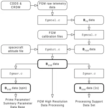
usu-F G M r a w t e l e m e t r y data fgmtel.c BF S data fgmcal.c BF S R data fgmhrt.c C D D S & C R D M F G M calibration files spacecraft attitude file B_{G S E} data fgmav.c fgmav.c

BG S E data (spin) BG S E data (1s)

Prime Parameter/ S u m m a r y P a r a m e t e r D a t a B a s e Processing Support Data Set F G M H i g h R e s o l u t i o n Data Processing

Fig. 8. Simplified flow diagram of the FGM data processing

soft-ware.

ally require additional calibration.

6 Data processing: summary of data throughput and data products

The data processing software routinely applied to the FGM data has the following main tasks:

– Transformation of the raw telemetry data into a format

suitable for further processing;

– Reconstruction of the time at which the vector data were

measured;

– Application of the calibration parameters to correct for

instrumental and other effects in the data in order to re-cover the accurate value of the magnetic field at the lo-cation of the sensors;

– Transformation of the magnetic field vectors into

stan-dard geophysical coordinate systems.

The data processing also performs the following additional tasks:

– Merging of the spacecraft position vectors to the

mag-netometer data streams;

– Averaging the measured magnetic field vectors over

dif-ferent time intervals;

– Providing appropriate data interfaces for the generation

Table 4. Calibration summary for the outboard sensor FGM SC1 FGM SC2 FGM SC3 FGM SC4 B0x −2.5 nT 0.0 nT −1.5 nT −14.0 nT B0y 4.0 nT −2.0 nT −5.0 nT −3.5 nT B0z 1.0 nT −0.5 nT −3.0 nT 4.5 nT 1B0x, 1B0y, 1B0z <0.2 nT γ x 0.7◦ 0.4◦ 0.8◦ 0.4◦ γ z 0.6◦ 0.7◦ 0.7◦ 1.2◦

Scale factors errors ∼0.1%

A simplified flow diagram of the FGM data processing software structure is shown in Fig. 8. The basic input to the processing comes from either the Cluster Data Dispo-sition System (CDDS) at ESOC, representing quick-look data, or from the Cluster Raw Data Medium (CRDM), the CDROMs used for the distribution of Cluster data. The mod-ular nature of the software is apparent in Fig. 8; the different modules implement the transformations enumerated and

de-scribed above. The modulefgmtel.cunpacks the

teleme-try and generates vectors in physical units in the (unorthog-onalised) sensor coordinate system. This module also gener-ates the timing and spin phase information for each measured

vector. The modulefgmcal.cincorporates the calibration

files, determined outside the processing chain, and generates the orthogonalised vectors in the spin-aligned coordinate

sys-tem. The following software module, fgmhrt.c, despins

the vectors, and, using the spacecraft attitude data, yields a time series in a selected geophysical system, normally in GSE, at the highest resolution in the current mode of the

instrument, according to BGSE using the notation from the

previous section of this paper. This is the form of the FGM software used to

BGSE=c(aut)−1BFSR

generate magnetic field data within the investigator team. Additional features (processing of the spacecraft position and

averaging, using thefgmav.cmodule) are used as

appro-priate.

The FGM magnetic field data are widely used by the Cluster investigator community, both to process their own data and for cooperative studies with the magnetometer team. Similarly, FGM data are also used in connection with ground-based investigations. The provision and distribution of magnetic field data represents a major effort undertaken by the FGM team to support the exploitation of the Cluster mission as a whole.

FGM data are routinely processed, using software sup-plied by the FGM team in the UK Cluster Data Handling Facility (UK-CDHF), a part of the Cluster Science Data Sys-tem (CSDS), to generate the spin-averaged (∼ 4 s resolution) Prime Parameter (PP) vector data from all four Cluster space-craft, as well as the Summary Parameter (SP) vector data from one spacecraft at a 1 min resolution. These data are

X

(R

)

0

5

10

15

Y

(R

)

10

15

20

3

4

1

₂

00 UT

10 UT

Fig. 9. Representation of the Cluster constellation in the X − Y

plane in the GSE coordinate system on 25 December 2000. The spacecraft constellation is shown magnified by a factor of 30.

then distributed through the CSDS to the other Cluster Data Centres, and to the Cluster scientific community. These data form the basis for most of the collaborative studies with the FGM team.

In addition, a number of Cluster investigations require FGM data at a higher 1 s resolution, for generating their own Prime Parameter data. A particular implementation of the FGM processing software has been made widely available to both CSDS Data Centres and to Cluster investigators, to generate the so-called Processing Support Data Set (PSDS). These data are used routinely for processing the data from other Cluster investigations, such as PEACE, CIS, EDI and EFW.

7 Overview of the early phase observations

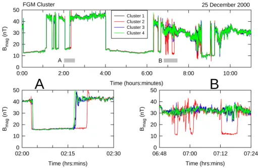
From its first commissioning operations in August 2000, Cluster and the FGM instruments on the four spacecraft demonstrated that the four-point measurements are able to bring a new understanding of magnetospheric phenomena. Due to the extended commissioning phase of the mission and all its instruments, routine four-spacecraft magnetic field measurements have only been available from Decem-ber 2000; once such measurements became available, it also became possible to address the scientific objectives of the mission. In the following, we present brief examples of mag-netic field measurements, demonstrating the capabilities and performance of the instrument. An early cusp crossing in August 2000 with simultaneous magnetic field observations was observed near perigee by three Cluster spacecraft (the fourth instrument had not yet been switched on). Routine observations of the outer cusp have been performed by Clus-ter since January 2001 (see Cargill et al., 2001). For initial bow shock studies, the sequence of crossings on 25 Decem-ber 2000 is particularly suitable. This series of shock

cross-Time (hours:minutes) 0:00 2:00 4:00 6:00 8:00 10:00 Bma g (nT) 0 10 20 30 40 50 Cluster 1 Cluster 2 Cluster 3 Cluster 4 FGM Cluster 25 December 2000 Time (hrs:mins) 02:00 02:15 02:30 Bma g (nT) 0 10 20 30 40 50 Time (hrs:mins) 06:48 07:00 07:12 07:24 Bma g (nT) 0 10 20 30 40 50 A B

A

B

Fig. 10. An overview of the multiple crossings of the bow shock by Cluster on 25 December 2000, with two intervals shown in higher

resolution to illustrate the motion and dynamics of the bow shock observed by Cluster.

ings is examined in more detail by Horbury et al. (2001). The orientation of the constellation was, at this time (near apogee), such that spacecraft 1, 3 and 4 were close to a plane perpendicular to the Earth-Sun line, while spacecraft 2 was sunward of the other three, between about 1100 and 1400 km, as shown in Fig. 9. Although during this period of the mission, the plasma instruments on Cluster remained switched off, it is possible to examine, in considerable detail, the variety of shock phenomena observed in these relatively low Mach number shocks for which the plasma beta param-eter (representing the ratio of the upstream plasma pressure to the magnetic field pressure) remained low, and the solar wind magnetic field remained relatively high (> 12 nT). An interesting feature of these shocks is that in spite of their ap-pearance as classical perpendicular bow shock waves when viewed at a resolution of 4 s, there is considerable structure associated with them, as seen at high resolution, which rep-resents fast dynamic processes, on time scales considerably shorter than their overall motion (Horbury et al., 2001). Fig-ure 10 illustrates the large-scale dynamics of the shock, as seen by the magnetometers on the four spacecraft.

Acknowledgements. The Cluster mission and the FGM team are

greatly indebted to many individuals who made the mission pos-sible and who contributed greatly to its success, as well as to the success of the FGM instrument. The rebirth of the mission, from the disaster of 1996, is due in the largest measure to the determi-nation of Prof. Roger Bonnet, ESA’s Director of Scientific Pro-grammes and of John Credland, ESA’s Head of Scientific Projects and previously Cluster Project Manager. We thank them also for partly funding the rebuilding of the FGM instruments. The Project Teams at ESA (in particular John Ellwood, Bodo Gramkow, Joseph Pereira, Colin Parkinson) and at Dornier, now Astrium (in partic-ular G¨unther Lehn, Roland Nord, Erwin Kraft) have greatly con-tributed to the successful rebuilding of the Cluster spacecraft and

their preparation for launch. We also remember the considerable contribution to Cluster by Gus Mencke and the late Hans Bach-mann. We are grateful to STARSEM for the successful and spectac-ular launches and to the Cluster Flight Operations Team at ESOC (in particular to Manfred Warhaut, Sandro Matussi and Colette Pullig) for their ready support of FGM operations. The support of the Clus-ter Project Scientists, first of Rudi Schmidt, laClus-ter of Philippe Escou-bet and Michael Faehringer is gratefully acknowledged. The rebuilt FGM instrument is very close to the original design developed by the earlier Technical Managers, Ray Carvell and John Thomlinson; the flight software still bears the imprint of its original designer, Ed Serpell. Also contributing to the hardware and calibration of the FGM were R. Kempen, H. K¨ugler, M. Rahm, I. Richter at the Tech-nische Universit¨at Braunschweig; J. Scheifele at the Goddard Space Flight Center; O. Aydogar at the Institut f¨ur Weltraumforschung, Graz. Special thanks are due to Mrs S. Balogh, Imperial College, for administrative and project support.

Financial support for the Cluster magnetic field investigation has been provided, in addition to ESA, by the Particle Physics and Astronomy Research Council in the United Kingdom (our special thanks to Mrs Sue Horne), DLR in Germany, the ¨Osterreichische Akademie der Wissenschaften in Austria and NASA in the United States (with special thanks to Dino Macchi).

References

Balogh, A., Cowley, S. W. H., Dunlop M. W., et al.: The Clus-ter magnetic field investigation: Scientific objectives and instru-mentation, in Cluster: mission, payload and supporting activities, ESA SP-1159, 95, 1993.

Balogh, A., Dunlop, M. W., Cowley, S. W. H., Southwood, D. J., Thomlinson, J. G., and the Cluster magnetometer team: The Cluster magnetic field investigation, Space Sci. Rev., 79, 65, 1997.

Balogh, A. and Dunlop, M. W.: FGM-specific multi-point analy-sis, Proc. Cluster II Workshop on Multiscale/Multipoint Plasma Measurements, ESA SP-449, 147–154, 2000.

Cargill, P. J., Dunlop, M. W., Balogh, A., and the FGM team: First Cluster results of the magnetic field structure of the mid- and high-altitude cusps, Ann. Geophysicae, (this issue) 2001. Dunlop, M. W., Woodward, T. I., Motschmann, U., Southwood, D.

J., and Balogh, A.: Analysis of non-planar structures with multi-point measurements, Adv. Space Res., 18, 8, 309–314, 1996. Dunlop, M. W., Woodward, T. I., Southwood, D. J., Glassmeier,

K.-H., and Elphic, R. C.: Merging 4 spacecraft data: Concepts used for analysing discontinuities, Adv. Space Res., 644, 1101–1106, 1997.

Dunlop, M. W. and Woodward, T. I.: “Discontinuity analysis: ori-entation and motion”, in: “Analysis Methods for Multispacecraft Data”, ISSI Science Report, SR-001, Kluwer Academic Pub-lisher, 1998.

Dunlop, M. W. and Woodward, T. I.: Cluster magnetic field analysis techniques, Proc. Cluster II Workshop on Multiscale/Multipoint Plasma Measurements, ESA SP-449, 351–354, 2000.

Dunlop, M. W., Balogh, A., Cargill P. J., and the FGM team: Cluster observes the Earth’s magnetopause: coordinated four-point mag-netic field measurements, Ann. Geophysicae, (this issue) 2001a. Dunlop, M. W., Balogh, A., Glassmeier K.-H., and the FGM team: Four-point application of magnetic field analysis tools: the cur-lometer and discontinuity analyser, Ann. Geophysicae, (this is-sue) 2001b.

Elphic, R. C.: Multipoint observations of the magnetopause: Re-sults from ISEE and AMPTE, Adv. Space Res., 8, 9, 223–238, 1988.

Fornacon, K.-H., Auster, H. U., Georgescu, E., Baumjohann, W., Glassmeier, K.-H., Haerendel, G., Rustenbach, J., and Dunlop, M. W.: The magnetic field experiment onboard Equator-S and its scientific possibilities, Ann. Geophysicae, 17, 1521–1527, 1999. Giacalone, J., Schwartz, S. J., and Burgess, D.: Artificial spacecraft in hybrid simulations of the quasi-parallel Earth’s bow shock: analysis of time series versus spatial profiles and a separation strategy for Cluster, Ann. Geophysicae, 12, 591–601, 1994. Glassmeier, K.-H., Motschmann, U., Dunlop, M. W., Balogh,

A., Acu˜na, M. H., Buchert, S., Carr, C. M., Fornacon, K.-H., Georgescu, E., Musmann, G., Schweda, K., and Vogt, J.: Cluster as a wave telescope: first results, Ann. Geophysicae, (this issue) 2001.

Horbury, T. S., Balogh, A., Lucek, E. A., Dunlop, M. W., and Cargill, P. J.: Cluster magnetic field observations of the bow-shock: motion, orientation and structure, Ann. Geophysicae, (this issue), 2001.

Kepko, E. L., Khurana, K. K., and Kivelson, M. G.: Accurate deter-mination of magnetic field gradients from four point vector

mea-surements: 1. Use of natural constraints on vector data obtained from a single spinning spacecraft, IEEE Transact. Magnetics, 32, 377, 1996.

Khurana, K. K., Kepko, E. L., Kivelson, M. G., and Elphic, R. C.: Accurate determination of magnetic field gradients from four point measurements: 2. Use of natural constraints on vector data obtained from four spinning spacecraft, IEEE Transact. Magnet-ics, 32, 5193, 1996.

Khurana, K. K., Kepko, E. L., and Kivelson, M. G.: Measuring magnetic field gradients from four-point measurements in space, AGU Monograph on Measurement Techniques, 1998.

Lucek, E. A., Dunlop, M. W., Horbury, T. S., Balogh, A., Cargill, P. J., Fornacon, K.-H., Oddy, T., and the FGM team: Cluster mag-netic field observations in the magnetosheath: four-point mea-surements of mirror structures, Ann. Geophysicae, (this issue), 2001.

Paschmann, G.: Magnetopause, cusp and dayside boundary layer: Experimental point of view, Proc. Cluster Workshop on Physical Measurements and Mission Oriented Theory, ESA SP-371, 149– 151, 1995.

Paschmann, G. and Daly, P.: Analysis Methods for Multispacecraft Data, ISSI Science Report, SR-001, (Eds), Kluwer Academic Publisher, 1998.

Russell, C. T.: Multipoint measurements of upstream waves, Adv. Space Res., 8, 9, 147–156, 1988.

Rezeau, L. Sahraoui, F., d’Humi`eres, E., Belmont, G., Cornilleau-Wehrlin, N., Mellul, L., Balogh, A., Robert, P., D´ecr´eau, P., and Canu, P.: A case study of low-frequency waves at the magne-topause, Ann. Geophysicae, (this issue) 2001.

Scholer, M.: Magnetopause, cusp and dayside boundary layer: The-oretical Point of view, Proc. Cluster Workshop on Physical Mea-surements and Mission Oriented Theory, ESA SP-371, 153–158, 1995.

Scholer, M. and Burgess, D.: The role of upstream waves in super-critical quasiparallel shock re-formation, J. Geophys. Res., 97, 8319–8326, 1992.

Southwood, D. J.: Multispacecraft measurements at varying scale-lengths – the Cluster/Regatta opportunity, Proc. Int. Workshop on Space Plasma Physics Investigations by Cluster and Regatta, ESA SP-306, 1–5, 1990.

Thomsen, M. F.: Multi-spacecraft observations of collisionless shocks, Adv. Space Res., 8, 9, 157–166, 1988.

Wild, J. A., Cowley, S. W. H., Davies, J. A., Khan, H., Lester, M., Milan, S. E., Provan, G., Yeoman, T. K., Balogh, A., Dunlop, M. W., Fornacon, K.-H., and Georgescu, E.: First simultaneous observations of flux transfer events at the high-latitude magne-topause by the Cluster spacecraft and pulsed radar signatures in the conjugate ionosphere by the CUTLASS and EISCAT radars, Ann. Geophysicae, (this issue), 2001.