Observations of the mesospheric semi-annual oscillation (MSAO) in water vapour by Odin/SMR

(1)

HAL Id: hal-00304210

https://hal.archives-ouvertes.fr/hal-00304210

Submitted on 30 May 2008

HAL is a multi-disciplinary open access

archive for the deposit and dissemination of sci-entific research documents, whether they are pub-lished or not. The documents may come from teaching and research institutions in France or abroad, or from public or private research centers.

L’archive ouverte pluridisciplinaire HAL, est destinée au dépôt et à la diffusion de documents scientifiques de niveau recherche, publiés ou non, émanant des établissements d’enseignement et de recherche français ou étrangers, des laboratoires publics ou privés.

Observations of the mesospheric semi-annual oscillation

(MSAO) in water vapour by Odin/SMR

S. Lossow, Jakub Urban, J. Gumbel, P. Eriksson, D. Murtagh

To cite this version:

S. Lossow, Jakub Urban, J. Gumbel, P. Eriksson, D. Murtagh. Observations of the mesospheric semi-annual oscillation (MSAO) in water vapour by Odin/SMR. Atmospheric Chemistry and Physics Discussions, European Geosciences Union, 2008, 8 (3), pp.10153-10187. �hal-00304210�

(2)

ACPD

8, 10153–10187, 2008 Observations of the MSAO in water vapour by Odin/SMR S. Lossow et al. Title Page Abstract Introduction Conclusions References Tables Figures ◭ ◮ ◭ ◮ Back Close

Full Screen / Esc

Printer-friendly Version Interactive Discussion

Atmos. Chem. Phys. Discuss., 8, 10153–10187, 2008 www.atmos-chem-phys-discuss.net/8/10153/2008/ © Author(s) 2008. This work is distributed under the Creative Commons Attribution 3.0 License.

Atmospheric Chemistry and Physics Discussions

Observations of the mesospheric

semi-annual oscillation (MSAO) in water

vapour by Odin/SMR

S. Lossow1, J. Urban2, J. Gumbel1, P. Eriksson2, and D. Murtagh2

1

Stockholm University, Department of Meteorology, Svante-Arrhenius-v ¨ag 12, 10691 Stockholm, Sweden

2

Chalmers University of Technology, Department of Radio and Space Science, H örsalsv ägen 11, 41296 G öteborg, Sweden

Received: 19 March 2008 – Accepted: 5 May 2008 – Published: 30 May 2008 Correspondence to: S. Lossow (stefan.lossow@misu.su.se)

(3)

ACPD

Full Screen / Esc

Abstract

Mesospheric water vapour measurements taken by the SMR instrument onboard the Odin satellite between 2002 and 2006 have been analysed with focus on the meso-spheric semi-annual circulation in the tropical and subtropical region. This analysis provides the first complete picture of mesospheric SAO in water vapour, covering

alti-5

tudes above 80 km where the only previous study based on UARS/HALOE data was limited. Our analysis shows a clear semi-annual variation in the water vapour distri-bution in the entire altitude range between 65 km and 100 km in the equatorial area. Maxima occur near the equinoxes below 75 km and around the solstices above 80 km. The phase reversal occurs in the small layer in-between, consistent with the downward

10

propagation of the mesospheric SAO in the zonal wind in this altitude range. The SAO amplitude exhibits a double peak structure, with maxima at about 75 km and 81 km. The observed amplitudes show higher values than the UARS/HALOE amplitudes. The upper peak amplitude remains relatively constant with latitude. The lower peak am-plitude decreases towards higher latitudes, but recovers in the Southern Hemisphere

15

subtropics. On the other hand, the annual variation is much more prominent in the northern hemispheric subtropics. Furthermore, higher volume mixing ratios during summer and lower values during winter are observed in the Northern Hemisphere sub-tropics, as compared to the corresponding latitude range in the Southern Hemisphere.

1 Introduction 20

The semi-annual oscillation (SAO) is the strongest mode of annual variability above 35 km altitude in the tropical region. This semi-annual variation has been first ob-served in temperature and zonal wind data in the 1960s (Reed and Rodgers, 1962; Reed, 1966). The oscillation peaks around the stratopause with amplitudes of around 30 m s−1 to 50 m s−1 in the zonal wind speed. At the stratopause maximum westerly

25

(4)

ACPD

Full Screen / Esc

observed in January and July. Subsequent measurements in the 1970s explored also altitudes above 60 km (Groves, 1972; Hirota, 1980). These measurements revealed that the semi-annual oscillation drops in amplitude above the stratopause and reaches a minimum around 65 km altitude. Higher up the SAO strengthens again, peaking a second time near the mesopause. This leads to a distinction between the stratospheric

5

(SSAO) and the mesospheric semi-annual oscillation (MSAO). The MSAO in the zonal wind has a similar amplitude and a phase which is approximately 180◦ out of phase with respect to the SSAO variations (Hirota, 1980; Hamilton, 1982).

The amplitude of the SAO usually decreases with increasing latitude, but can recover in the subtropics depending on altitude. In this regard, the semi-annual oscillation

ex-10

hibits a latitudinal asymmetry, with higher amplitudes in the Southern Hemisphere sub-tropics (Belmont and Dartt, 1973; Ray et al., 1997). Besides this latitudinal asymmetry, the semi-annual oscillation shows also a seasonal asymmetry with stronger zonal wind variations during the first cycle, which starts with the easterly phase of the zonal wind in the Northern Hemisphere winter time (Delisi and Dunkerton, 1988; Garcia et al.,

15

1997).

Early attempts of explaining the semi-annual oscillation used the semi-annual varia-tion of the solar radiavaria-tion in the tropics as a possible cause (Webb, 1966). Further in-vestigations showed rather soon that the solar forcing is not sufficient enough to create the SAO signature in the zonal wind (Meyer, 1970). The forcings that cause the easterly

20

and westerly mean flow accelerations in the stratospheric SAO are rather different in nature. The easterly accelerations, on one hand, are due to the meridional advection of easterlies from the summer hemisphere across the equator (Meyer, 1970; Holton and Wehrbein, 1980). This effect occurs twice a year and peaks right after solstice. Another contribution to the easterly accelerations arises from the eddy momentum deposition

25

by breaking planetary waves which have been ducted in the tropics. The westerly ac-celerations, on the other hand, are thought to be due to vertically propagating ultra-fast Kelvin waves and internal gravity waves that interact with the mean flow and deposit their momentum in the upper stratosphere. The relative portions of these two wave

(5)

ACPD

Full Screen / Esc

contributions has been discussed extensively (Hitchman and Leovy, 1988; Hamilton et al., 1995; Sassi and Garcia, 1997). The forcing of the mesospheric SAO is more uncer-tain. In general, the forcing is attributed to a broad spectrum of vertically propagating gravity and high-speed Kelvin waves, excited in the lower atmosphere. These waves are filtered by the zonal mean wind variations in the stratospheric SAO. This allows only

5

waves with the opposite horizontal propagation direction with respect to the zonal wind direction to propagate further upward into the mesopause region, where these waves usually break. The filtering of these waves accounts for the phase shift between the stratospheric and mesospheric SAO (Dunkerton, 1982; Hitchman and Leovy, 1986).

The asymmetry between the two cycles of the semi-annual circulation is attributed

10

to differences in the extratropical planetary wave forcing (Delisi and Dunkerton, 1988). The latitudinal asymmetry in the subtropics has been investigated in detail by Ray et al. (1998). According to their work no single forcing contributing to the SAO could be clearly connected to this asymmetry. The largest contribution arose instead from a different phasing of the maximum meridional advection between both hemispheres,

15

which takes place later in the Southern Hemisphere.

The annual variation in the zonal wind influences also the annual distribution of at-mospheric trace gases via induced meridional and vertical transport. The stratospheric SAO in water vapour has for example been observed by the MLS (Microwave Limb Sounder, Barath et al., 1993) and the HALOE (Halogen Occultation Experiment,

Rus-20

sell et al., 1993) instrument, both onboard the Upper Atmosphere Research Satel-lite (UARS) (Carr et al., 1995; Randel et al. 1998; Jackson et al., 1998). Signatures of the stratospheric SAO could be observed above 20 hPa (∼27 km). The analysis of these data sets showed a maximum amplitude of 0.2 ppmv slightly below 1 hPa (∼48 km), with water vapour minima in February and August and maxima in May and

25

November, respectively. The mesospheric SAO in water vapour has so far only been addressed by Jackson et al. (1998), based on HALOE measurements between the end of 1991 and the beginning of 1996. Compared to the SSAO, the MSAO exhibits a much stronger amplitude. Above the described SAO minimum at around 65 km the

(6)

am-ACPD

Full Screen / Esc

plitude of the mesospheric SAO in water vapour increases rapidly, peaking at around 0.01 hPa (∼80 km) with more than a half ppmv. In accordance with the phase shift between the MSAO and the SSAO the annual water vapour distribution shows min-ima around April/May and October/November and maxmin-ima around January/February and July/August. The rapid increase of SAO amplitude in the middle and upper

meso-5

sphere is mainly associated with the strong vertical gradient in water vapour in that altitude range. The UARS/HALOE water vapour measurements also showed the latitu-dinal asymmetry of the MSAO in the subtropics. In the Northern Hemisphere the SAO exhibited maximum amplitudes of about 0.25 ppmv between 30◦and 35◦latitude, while in the same latitude band in the Southern Hemisphere the amplitudes showed peak

10

values up to 0.6 ppmv at an altitude close to 80 km.

The Sub-Millimetre Radiometer (SMR, Frisk et al., 2003) onboard the Odin satel-lite passively scans thermal emission of several trace gases at the atmospheric limb (Murtagh et al., 2002). Measurements at 557 GHz provide global fields of mesospheric water vapour up to an altitude of 100 km. In this paper we present water vapour

ob-15

servations in the tropics between 2002 and 2006. This data set has been analysed with particular focus on the mesospheric semi-annual circulation in water vapour. The Odin/SMR data provide a complete picture of the MSAO signal, with new insights in particular above 80 km altitude, where the HALOE based analysis of the MSAO was limited.

20

The outline of the paper is as follows. In Sect. 2 we give an general overview of the mesospheric water vapour observations by Odin/SMR and describe their quality and handling. The observations of the mesospheric SAO are presented and analysed in Sect. 3 and the results are discussed in Sect. 4.

2 Odin/SMR observations of mesopheric water vapour

25

The Odin satellite has been launched on 20 February 2001 into a polar, sun syn-chronous and near-terminator orbit at an altitude of around 600 km. Odin is orbiting the

(7)

ACPD

Full Screen / Esc

Earth about 15 times a day, passing the equator at approximately 18:00 LT on the as-cending note. One of two instruments carried onboard the satellite is the Sub-Millimetre Radiometer. This instrument is a heterodyne receiver employing a 1.1 m telescope in order to passively measure thermal emission at the atmospheric limb. It is com-posed of four tuneable sub-millimetre radiometers covering frequency ranges between

5

486 GHz and 581 GHz and one millimetre radiometer measuring around 119 GHz. Two autocorrelators and one acousto-optical spectrograph can be attached to any of the radiometers to detect the received signal (Frisk et al., 2003).

2.1 Measurements of the 557 GHz band and its retrieval

Odin/SMR measures several atmospheric emission lines of water vapour and its

iso-10

topes (Urban et al., 2007). Measurements of the 557 GHz band have been performed on 4 days per month for the greater part of the Odin aeronomy mission. In April 2006 the measurement frequency was increased to 7 days per month. Since May 2007 these measurements are performed every second day. These measurements are part of a stratosphere/mesosphere mode, where the atmospheric scans in general are ranging

15

from 7 km to 110 km altitude. With a scanning velocity of 0.75 km s−1_{it takes more than} two minutes to complete such a stratosphere/mesosphere scan. Thus around 40 to 45 scans in total are performed per orbit. The integration time for a single tangent height measurement is approximately 1.85 s. This time in combination with the spectrom-eter read-out times and the antenna characteristics dspectrom-etermines the effective altitude

20

resolution of the measurements, which is in the order of around 3 km. The horizon-tal resolution in this altitude layer is characterised by the path length, which is about 400 km. The horizontal sampling is given by the movement of the satellite, which is ap-proximately 7 km/s projected on the ground, and the time needed to perform the scan. Accordingly, the horizontal sampling is typically about one measurement per 1000 km.

25

For the measurements of the 557 GHz band two of the four radiometers are used, ei-ther the 549A1 radiometer (covering 541 GHz to 558 GHz) or the 555B2 radiometer (covering 547 GHz to 564 GHz), using in total three different frequency configurations.

(8)

ACPD

Full Screen / Esc

In either case autocorrelator number 1 is attached as the signal receiving spectrometer. The water vapour emission line covered by the measurements is centred at 556.936 GHz.

This line is the strongest water vapour emission line in the entire microwave region. The line is optically thick in the centre up to approximately 70 km to 75 km. Water

5

vapour profiles can be retrieved from the spectra covering the altitude range between 40 km and 100 km. The limiting factor on the lower altitude end is a combination of the limited bandwidth of the SMR instrument of 800 MHz and the high optical thickness even in the line wings. The upper altitude limit is given by the signal-to-noise ratio and the volume mixing ratio of water itself. The retrieved altitude resolution is usually about

10

3 km. The retrieval is done with a non-linear scheme using the Optimal Estimation Method (OEM) (Rodgers, 2000; Baron et al., 2001). The iteration scheme is based on a Newton and Levenberg-Marquardt method (Lauti ´e et al., 2001). The typical retrieval precision of the water vapour volume mixing ratio for a single scan is between 5% and 15% below 80 km. Above 90 km the retrieval precision can easily exceed 50%. For

15

more detailed information about the Odin/SMR mesospheric water vapour retrieval the reader is referred to Urban et al. (2007) and Lossow et al. (2007).

2.2 Data quality

The aim of the following quality assessment is to give a sincere characterisation of the mesospheric Odin/SMR water vapour data in the tropical and subtropical region.

20

For the current study we use the official Odin/SMR retrieval version 2.1, produced at the Chalmers University of Technology in G ¨oteborg, Sweden. The changes and status of this retrieval version for the mesospheric water have been described by Lossow et al. (2007). The quality of the Chalmers v2.1 level-2 data on the global scale has been assessed by a comparison to correlative satellite measurements performed by the

25

Fourier Transform Spectrometer (FTS) instrument onboard the Canadian ACE/SCISAT-1 satellite (Bernath et al., 2005). ACE/FTS measures extinction spectra in the mid-infrared, using the rather precise solar occultation technique. The water vapour

(9)

pro-ACPD

Full Screen / Esc

files have been retrieved using the ACE/FTS retrieval version 2.2 (Boone et al., 2005). The results of mesospheric ACE/FTS water vapour retrieval have already been com-pared to the EOS MLS (Earth Observing System Microwave Limb Sounder) instrument (Waters et al., 2006) onboard the Aura satellite, showing a very good agreement with deviations of less than 5% below 85 km (Lambert et al., 2007). The comparison of the

5

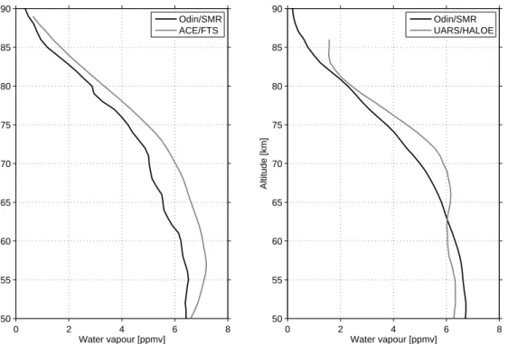
mesospheric water vapour retrievals between Odin/SMR and ACE/FTS exhibits on the global perspective a dry bias of the SMR data in the entire altitude region (Carleer et al., 2008). The observed behaviour is very similar in the latitude range between 40◦_S and 40◦N, which we implement in this study. This can be seen in the left panel of Fig. 1, which shows a comparison of mean profiles based on 118 events in this latitude range

10

where Odin/SMR and ACE/FTS measurements were not separated by more than 5 h in time and 1000 km in space. At 50 km Odin/SMR exhibits 0.2 ppmv (∼3% deviation with respect to the mean of Odin/SMR and ACE/FTS) less water vapour than ACE/FTS. The dry bias increases above, peaking with 1.1 ppmv (∼20% deviation) in the altitude range between 60 km and 70 km. Above this altitude range the deviation decreases with

alti-15

tude and between 80 km and 89 km (the uppermost altitude retrieved by ACE/FTS) the Odin/SMR dry bias is always below 0.5 ppmv (∼20%–40% deviation).

The SAO analysis of UARS/HALOE data by Jackson et al. (1998) is an important basis for the discussion of the Odin/SMR observations of the semi-annual oscillation (Sect. 4). Therefore, we have performed the same kind of comparison for the tropical

20

and subtropical latitude region between these two instruments as we did with ACE/FTS before. The results of this comparison are shown in the right panel of Fig. 1. In this case we found 771 events of coincident measurements. Below 60 km the retrieved water vapour from Odin/SMR measurements is 0.3 ppmv (∼5% deviation with respect to the mean of Odin/SMR and UARS/HALOE) higher as compared to UARS/HALOE.

25

At 62 km altitude both instruments show the same amount of water vapour. Above this altitude the retrieved Odin/SMR water vapour shows a dry bias, similar as seen in the comparison with ACE/FTS. This bias maximises at around 72 km with 1.0 ppmv (∼18% deviation) and above to about 0.3 ppmv (∼5% deviation) at 80 km altitude.

(10)

ACPD

Full Screen / Esc

For the analysis of the semi-annual oscillation we expect in general no or only a very small influence of the negative bias of the SMR data set in the altitude range of interest. This conclusion is based on our idea to analyse the SAO signal as a temporal deviation around a mean state.

2.3 Data set and its handling

5

For the characterisation and analysis of the mesospheric semi-annual oscillation in water vapour we use measurements from Odin/SMR performed between 2002 and 2006. Only data taken by the frequency configuration “freqmode 19” has been imple-mented in this analysis. This frequency configuration employs the 549A1 radiometer and has been used continuously and most often throughout the whole time period for

10

the mesospheric water vapour measurements. Moreover, this configuration is the most optimised out of the three frequency configurations used for those measurements (see Sect. 2.1). We implement only profiles which have been flagged as usable for scien-tific analysis by the retrieval quality control. This quality control is based on different parameters, such as the convergence, the cost function of the retrieval (chi-square

sta-15

tistical analysis), the Levenberg-Marquardt parameter (regularisation of the non-linear retrieval) and the retrieved pointing offset. From those profiles only data are used, where the measurement shows a response of at least 70% in the retrieved values. This high measurement response ensures that the influence of the a priori information needed for an OEM retrieval is minimised.

20

Due to its sun-synchronous orbit Odin always performs measurements only at two distinct local times (LT) at a given latitude (one local time on the ascending and the second one on the descending node). In the equatorial and tropical region Odin takes measurements around 06:00–07:00 LT and 18:00–19:00 LT. Thus, any given result would only represent the characteristics for these two local time ranges. In order to

25

get general results the local time variation must be accounted for, which is determined by tides. Tidal contributions to the data set can be significant, especially in the up-per mesosphere and lower thermosphere, and can influence the analysis of the

(11)

semi-ACPD

Full Screen / Esc

annual oscillation. In the tropical region the most prominent tide is the migrating diurnal tide, which propagates westwards following the apparent motion of the Sun (e.g. Chap-man and Lindzen, 1970; Forbes, 1995). This tide is mainly forced in the troposphere by solar heating and exhibit, like the SAO, a semi-annual variation with peaks near the equinoxes (Vincent et al., 1988; Burrage et al., 1995; McLandress et al. 1997).

5

In addition, a weaker migrating semi-diurnal tide and non-migrating tides can be ob-served. Measurements of the tidal variation of water vapour in the altitude range of interest are very rare and reports in the literature are essentially non-existing. Due to its sun-synchronous orbit, Odin measurements are not suitable to provide informa-tion on the diurnal variainforma-tion of water vapour. Similarly satellite-based solar occultainforma-tion

10

instruments have only a limited capability to extract the diurnal characteristics, since they only measure at sunset and sunrise. Data from ground-based radiometers usually needs to be integrated over 24 h in order to provide useful measurements at an altitude of 80 km. Hence, for the time being, only models can give answers about the diurnal (tidal) variation of water vapour in the upper mesosphere and lower thermosphere. In

15

our case we used data from WACCM (Whole Atmosphere Community Climate Model; Garcia et al., 2007) in order to estimate the most important tidal contributions in the tropics and subtropics due to the migrating diurnal and semi-annual tide. In the tropical region the maximum amplitude of the migrating diurnal tide is about 1 ppmv, while the migrating semi-diurnal tide reaches a maximum amplitude of 0.4 ppmv. According to

20

the model the tidal contributions are rather small at around 06:00 LT and 18:00 LT. The modelled tidal contributions as a function of latitude, local time, altitude and day of year have been subtracted from the individual water vapour profiles retrieved before any averaging. This correction does neither take into account non-migrating tides nor the inter-annual variation of migrating tides due to quasi-biennial oscillation (QBO, Baldwin

25

et al., 2001, and references therein) (Burrage et al., 1995).

After the tidal correction has been applied the data set has been averaged onto a 15 day time grid, where every grid point describes a mean of 30 days. Thus the single data points are not completely independent from each other in time. In the vertical

(12)

ACPD

Full Screen / Esc

the data have been interpolated onto a 1 km altitude grid. In order to describe the latitudinal dependence of the SAO the data have been averaged over a latitude range of 10◦_{using a 5}◦_{latitude grid. Hence, just as in the time domain, the single data points} are not independent from each other in the latitude domain.

The amplitudes of the semi-annual and annual variation of the mesospheric water

5

vapour distribution in the tropical and subtropical region are then determined by means of a wavelet analysis. In order to get general results we averaged over the time com-ponent of the global wavelet spectrum (Torrence and Compo, 1998). For this spectral analysis we have employed the whole time series between 2002 and 2006. A data gap in February 2006 has been filled by linear interpolation for the sake of convenience.

10

In order to estimate the statistical significance of the determined amplitude we applied the jackknife method (Efron, 1979). The basic idea behind this method is to systemati-cally recalculate the amplitude of the desired frequency components from altered time series, where in each case a different set of observations has been removed from the original time series. This procedure leads to a new data set of amplitudes, which can

15

be used to estimate the standard deviation of the amplitude derived from the original time series.

3 Observations and results

3.1 Equatorial region 10◦S–10◦N

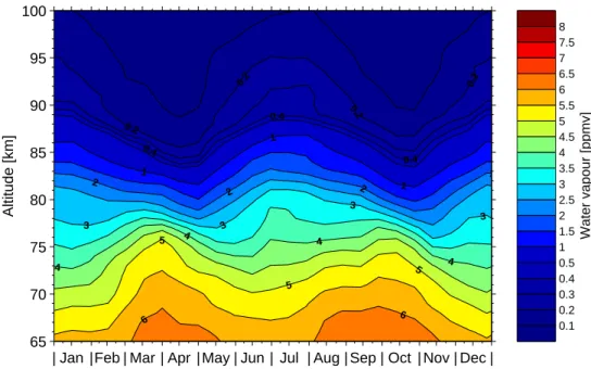
Figure 2 shows the mean annual water vapour distribution in the latitude range between

20

10◦S and 10◦N as measured by Odin/SMR for all years considered. At all altitudes a semi-annual variation of water vapour can be observed. In the upper altitude range above 80 km water vapour exhibits maxima at the end of December/beginning of Jan-uary and in July. The minima occur in April and October. In the lower altitude range below 75 km, on the other hand, the position of the maxima and minima is flipped

25

(13)

ACPD

Full Screen / Esc

March/beginning of April and in October while the minima appear in December and at the turn of June and July. The transition between the these two different phase domains occurs in a rather thin layer between approximately 75 km and 80 km.

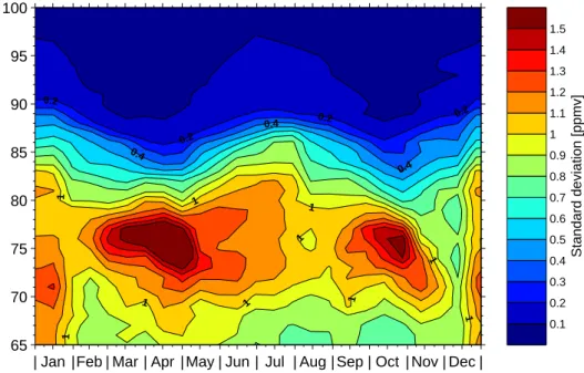
The standard deviation of the mean water vapour distribution is given in Fig. 3, in order to give also an indication of the observed annual and inter-annual variability. The

5

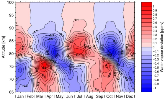
variability exhibits in general the same pattern as the mean water vapour distribution. The absolute highest variability can be observed at about 75 km around the equinoxes. Figure 4 shows the deviation of the mean annual water vapour distribution shown in Fig. 1 with respect to a 180 days running average of this mean distribution. This figure shows more clearly the observed time shift of the water vapour extrema between 75 km

10

and 80 km. In addition these deviations provide also a first indication of the amplitude of the semi-annual variation of water vapour. The absolute maximum amplitudes occur in two layers, one at about 75 km and the other one at around 81 km, clearly exceeding 0.5 ppmv. Above 90 km the absolute water vapour deviations are small, just like the absolute water vapour volume mixing ratio itself. Below 75 km the absolute deviations

15

decrease with decreasing altitude.

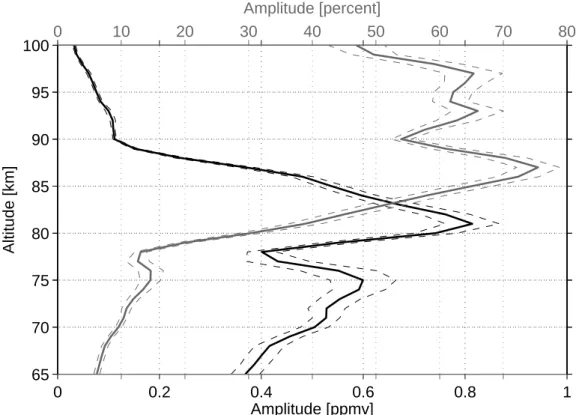
The absolute amplitude of the semi-annual variation of the water vapour distribution as a function of altitude is given by the black line in Fig. 5 (using the lower axis). As already evident from Fig. 4, the semi-annual variation of the mesospheric water vapour distribution peaks at two distinct altitudes, namely at 75 km with around 0.6 ppmv and

20

at 81 km with around 0.8 ppmv. In the altitude region in-between, where also the phase shift of the semi-annual variation occurs, a significant minimum can be observed. The amplitude of the semi-annual component drops here to 0.4 ppmv at 78 km altitude. In the altitude range between 81 km and 90 km the amplitude decreases rapidly, where also the absolute amount of water vapour falls off rather fast. At 90 km altitude the

25

amplitude of the semi-annual component is somewhat more than 0.1 ppmv. Above 90 km the amplitude decreases much slower with altitude. It is also notable that we do not observe a distinct altitude where the minimum amplitude of the semi-annual variation between the stratopause and the higher mesosphere occurs. The minimum

(14)

ACPD

Full Screen / Esc

amplitude we observe is in the order of 0.30 ppmv to 0.35 ppmv and spans over the altitude range between 50 km and 63 km (not shown here).

Expressed in relative terms the semi-annual variation peaks above 80 km as shown by the grey line in Fig. 5 (using the upper axis). As reference we used the mean profile derived from the annual distribution displayed in Fig. 2. Two maxima can be observed

5

above 80 km, where the relative amplitude of semi-annual variation is up to 60% and more. One maximum occurs close to 87 km and a second one is spread out over the altitude range between approximately 93 km and 97 km. These two maxima are separated by a minimum at 90 km. At this altitude the amplitude of the semi-annual variation stands for somewhat more than 50% of the total water vapour amount. Below

10

85 km the relative amplitude decreases strongly with decreasing altitude. At 78 km the relative amplitude of the semi-annual variation is less than 15%. Even below this altitude the amplitude continues to decrease with decreasing altitude, but only slightly. A comparison with the data where the tidal contributions were not removed using WACCM revealed no significant differences with respect to the amplitude of the

semi-15

annual component of the mesospheric water vapour variation.

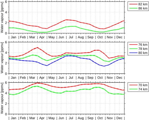
Figure 6 gives a detailed view on some of the mean annual water vapour time series in the three key altitude ranges. The lower panel shows time series below 75 km. The altitude range between the two amplitude maxima of the semi-annual variation, 76 km and 80 km, where also the phase shift of the SAO occurs, is given in the middle panel.

20

Time series from above 81 km are shown in the upper panel. In the altitude range below 75 km the first annual minimum (starting in January) exhibits in general a lower water vapour concentration than the second one. On the contrary the first annual maximum tends to show slightly more water vapour with respect to the maximum in the Northern Hemisphere autumn. The second maximum appears to be “broader” in time. At 76 km

25

a small bump can be observed at the end of June/beginning of July. This bump may be a very first indication of the phase change of the semi-annual variation occuring in the thin layer above. Two kilometres higher up the annual variation looks like as having rather three maxima than only two. One maximum occurs in March, one in December

(15)

ACPD

Full Screen / Esc

and a very broad one that is spread out between July and September. At 80 km altitude the phase shift of the semi-annual water vapour variation is almost complete. Above this altitude, in general more water vapour can be observed at the maximum in the middle of the year as compared to the maximum at the end of the year. As evident in Figs. 2 and 4, Fig. 6 clearly manifests that the phase of the semi-annual variation of

5

water vapour below 75 km and above 81 km is not completely shifted by 180◦, since the corresponding extrema lie not perfectly on top of each other.

3.2 Tropical and subtropical region 35◦S–35◦N

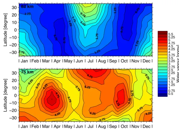
Two latitudinal cross section examples of the mean annual water vapour distribution are given in Fig. 7, covering the latitude range between 35◦S and 35◦N. The lower

10

panel shows the altitude of 75 km and the upper panel shows the altitude of 83 km respectively. At 75 km altitude, the water vapour maxima both in March/April and in September/October appear to be centred in the Southern Hemisphere at about 5◦S. From the centre of the maximum towards the mid-latitudes the amount of water vapour generally decreases and the strength of the semi-annual variation gets weaker. The

15

water vapour distribution in the extra tropical mesosphere is dominated by an annual component. Maximum values occur during summer time and the minimum can be observed in winter. This behaviour is due to a gravity wave driven meridional circulation with an ascending branch over the summer hemisphere and down-welling motion over the winter hemisphere. Parts of this annual component become evident at latitudes

20

higher than 25◦ _{shown in Fig. 7. At those latitudes also inter-hemispheric differences} can be noted. In comparison to its southern hemispheric counterpart the northern summer exhibits higher water vapour volume mixing ratios. On the contrary less water vapour can be observed in the northern winter than in the Southern Hemisphere winter. The structure of the water vapour distribution looks simpler at 83 km than at 75 km,

25

since the water vapour extrema occur at the same time at all latitudes. The observed maxima in the tropical region could literally be described as the “tips of two tongues”, originating as an equatorward extension of the extra-tropical summer water vapour

(16)

ACPD

Full Screen / Esc

maximum in each hemisphere. Similar to the conditions at 75 km seasonal inter-hemispheric differences can clearly be observed at the latitude higher than 25◦_{. In} addition, looking for example at the 1.75 ppmv contour line it can be seen that this line extends from the Northern Hemisphere down to a latitude of about 20◦S in the Northern Hemisphere summer. On the other hand, this contour line extends from the

5

Southern Hemisphere only up to a latitude slightly north of the equator in the Southern Hemisphere summer. This observation can also be made, even if not so clear, using other contour lines. A similar behaviour can be observed up to an altitude of 90 km.

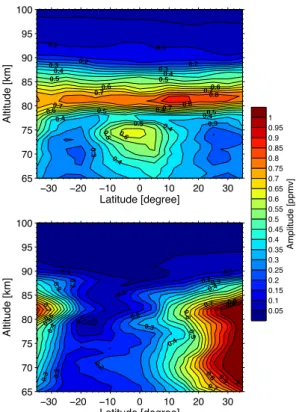
Figure 8 gives an overall picture of the latitude and altitude dependence of the am-plitude of the semi-annual and annual variation of the mesospheric water vapour

distri-10

bution. Above approximately 78 km the amplitude of the semi-annual variation exhibits nearly no latitude dependence within the latitude range between 35◦S and 35◦N. The maximum amplitude can be observed at around 82 km at a latitude of circa 15◦N ex-ceeding 0.85 ppmv. This observation is not statistically significant, since the amplitude error determined by the jackknife method is also high. The same significance

prob-15

lem applies to amplitude maximum at 75 km, which appears to be slightly centred on the Southern Hemisphere. Towards higher latitudes the amplitude of the semi-annual water vapour variation decreases, reaching a minimum at around 25◦_{latitude with} ap-proximately 0.25 ppmv. In the altitude range between 65 km and 75 km the amplitude increases again, but only in the Southern Hemisphere. This increase is rather strong

20

especially at the higher altitudes where for example an amplitude of 0.5 ppmv at 75 km can be observed at 35◦S.

The amplitude of the annual component of the variation of the mesospheric water vapour distribution reveals a clear inter-hemispheric difference with the minimum cen-tred in the Southern Hemisphere in the latitude range between 5◦S and 20◦S. The

25

minimum amplitude here is rather constant with altitude, usually between 0.1 ppmv and 0.15 ppmv, except for the uppermost altitudes above 90 km. The strongest latitude dependence of the annual component in the Southern Hemisphere occurs in a layer between 80 km and 85 km where the amplitude increases up to more than 0.8 ppmv

(17)

ACPD

Full Screen / Esc

at 35◦_{S. South of 30}◦_{S between 65 km and 90 km the amplitude of the annual water} vapour variation is comparable to the amplitude of the semi-annual variation. At lower southern latitudes the semi-annual variation is in contrast clearly the dominant variation in this altitude range. In the Northern Hemisphere the amplitude of the annual variation of the water vapour distribution increases rather strong towards the mid-latitudes,

espe-5

cially below 85 km. At 35◦N the amplitude exceeds 1 ppmv in that altitude range. The transition from the semi-annual to the annual variation as the dominant contribution to the temporal variation of the water vapour distribution occurs at approximately 10◦_N, concerning the altitude range between 65 km and 85 km. Above 90 km the amplitude of the annual water vapour variation exhibits nearly no latitude dependency. At those

10

altitude the semi-annual variation is stronger as the annual variation amplitude at all latitudes implemented in our analysis. In addition to semi-annual and annual variations described here we also found a small QBO and a 90 day time variation.

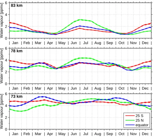
In Fig. 9 some examples of time series at 25◦_{N (green) and 25}◦_{S (red) provide a} more closer look at the two hemispheres and differences between them, as described

15

in the last two figures, i.e. Figs. 7 and 8. Just for the sake of comparison we also in-cluded the time series at the equator (blue). The results are shown at 73 km (lower panel), 78 km (middle panel) and 83 km (upper panel). The time series at 73 km in the Northern Hemisphere exhibits clearly a dominating annual component of the water vapour variation. At 25◦_{S the semi-annual variation is still the prevailing component.} 20

Like at the equator in both hemispheres the water vapour maxima around the equinox in March due to the semi-annual variation can still be detected. 5◦_{more polewards this} peak can rather hardly be observed. It is notable the water vapour distribution at 25◦_S does not exhibit a minimum around July, that means local winter, as expected from the semi- and annual variation. This behaviour is not as obvious in the Northern

Hemi-25

sphere but is based on the observation that the phase shift at the subtropical latitudes starts already at an altitude of about 65 km to 70 km. The water vapour structure at 78 km and the described characteristics are relatively similar to those at 73 km. As a prominent deviation also the maximum at the equinox at the end of September can be

(18)

ACPD

Full Screen / Esc

distinguished on both hemispheres. This is even visible at 30◦ _{latitude. In the} South-ern Hemisphere clear signatures of the phase shift of the semi-annual variation at that altitude can be observed. This phase shift exists also in the Northern Hemisphere, but is more hidden due to the dominating annual component of the water vapour variation at that latitude. At 83 km the water vapour distribution shows a semi-annual variation

5

combined with a strong annual component in both hemispheres. As noted before the summer maximum is stronger in the Northern Hemisphere, while the winter maximum is stronger in the Southern Hemisphere. This behaviour is most obvious here, but can easily be observed also at 73 km and 78 km.

4 Discussion and summary

10

Five years (2002–2006) of Odin/SMR measurements of the mesospheric water vapour distribution in the tropical and sub-tropical region were used to give a general picture of the mesospheric semi-annual oscillation in water vapour. Year to year variability of the MSAO is clearly observable in Fig. 3. This variability is associated with the modulation of the SAO by the quasi-biennial oscillation (Garcia et al., 1997; Mayr et al. 1997).

15

A detailed analysis of the inter-annual variability and the signal of the quasi-biennial oscillation signal in mesospheric water vapour distribution measured by Odin/SMR will be the subject of a future study.

Our data set shows distinct signatures of the semi-annual oscillation in the equatorial region in the entire altitude range of interest, namely between 65 km and 100 km. The

20

most prominent feature is a phase shift in the semi-annual variation, which occurs in the altitude range between approximately 75 km and 80 km. This feature can also be observed in the temperature distribution, where the transition occurs somewhat higher in altitude (Clancy et al., 1994; Remsberg et al., 2002; Shepherd et al., 2004; Huang et al., 2006). Below this thin transition layer the maxima of the water vapour distribution

25

are found around the equinoxes, while they occur around the solstices above this layer. Noticeable is also that the phase shift is not entirely 180◦ between these two altitude

(19)

ACPD

Full Screen / Esc

domains. In comparison to the HALOE analysis of the mesospheric SAO in water vapour (Jackson et al., 1998; their Fig. 3) the maxima observed by Odin/SMR occur one month earlier. A recent model study of the SSAO in water vapour by Lelieveld et al. (2007) make a similar observation, when comparing their results to UARS/HALOE data. This is very likely explained by an under-sampling of the HALOE data due to

5

the solar-occultation technique and the UARS orbit. Part of the data are separated by 60 to 80 days and have subsequently over-smoothed onto a 30 day mean grid. The observed phase shift of the semi-annual variation of the water vapour distribution between 76 km and 80 km is consistent with the downward propagation of the MSAO in the zonal wind in this altitude range. In general, the mesospheric SAO in water

10

vapour can be associated to vertical and meridional transport, induced by the MSAO in the zonal wind. This comprises down-welling and adiabatic warming starting at the onset of the easterlies on one hand and upward motion with corresponding adiabatic cooling occuring at the onset of the westerlies on the other hand (Hirota, 1980; Garcia et al. 1997). In the equatorial region the amplitude of the mesospheric SAO exhibits

15

a double peak structure with one maximum at 75 km and another one at 81 km. The mean amplitudes of these peaks are with 0.6 ppmv and 0.8 ppmv respectively. Both amplitudes vary by ±0.3 ppmv over the years, as discussed before in terms of inter-annual variability. This observed structure of the SAO amplitude resembles in principle the amplitude pattern observed by UARS/HALOE (Jackson et al., 1998; their Fig. 5).

20

Since their analysis is limited to 80 km the upper peak can not be observed completely and accordingly the full amplitude is unknown. Furthermore, the minimum between the two maxima is not statistically significant in the UARS/HALOE evaluation. The amplitude of the lower peak at 75 km and also the amplitudes observed at the altitudes below are smaller in the HALOE analysis. The authors discuss the possibility of an

25

underestimation based on the aforementioned over-smoothing in time of the HALOE data. The analysis of the Odin/SMR data shows that the amplitude at the node between stratospheric and mesospheric SAO does not decrease to zero and that the node is actually spread out over a broader altitude range between 50 km and 63 km. Even very

(20)

ACPD

Full Screen / Esc

high altitudes show a clear SAO signal, being actually strongest above 85 km in terms of the relative variation of the volume mixing ratio.

With respect to the latitudinal behaviour of the tropical/subtropical MSAO in water vapour we need to distinguish between the two altitude regions below and above 78 km. The amplitude of the SAO below 78 km decreases towards higher latitudes, reaching

5

a minimum amplitude at about 25◦ latitude. This picture is consistent with the HALOE observations. As before, the amplitudes observed by Odin/SMR are higher than the amplitudes derived from the HALOE observation. The amplitude of the SAO above 78 km on the other hand does not show any significant variation with latitude. A similar behaviour has been observed for the SAO in temperature by the WINDII (Wind Imaging

10

Interferometer, Shepherd et al. 1993) instrument onboard the UARS satellite (Shepherd et al., 2004). Correspondingly, the amplitude of the mesospheric semi-annual oscilla-tion in water vapour exhibits a single peak structure at latitudes higher than 20◦. In the Southern Hemisphere the amplitude of the SAO recovers at sub-tropical latitudes below 80 km. This effect has also been observed in the UARS/HALOE analysis of the

15

mesospheric SAO in water vapour (Jackson et al., 1998) and is in agreement with the characteristics of the SAO in the zonal wind (Ray et al., 1997). Also the annual com-ponent of the water vapour variation shows clear inter-hemispheric differences in the subtropics with a higher amplitude in the Northern Hemisphere. The minimum ampli-tude of the annual component is found in the Southern Hemisphere between 5◦_{S and} 20

20◦_{S. The evaluation of the HALOE water vapour data by Jackson et al. (1998) shows} the amplitude minimum at about 5◦S and thus somewhat more equatorward than for Odin/SMR. The amplitudes of the annual oscillation derived from the UARS/HALOE data are again smaller, as discussed earlier. The observations of latitudinal structure of the annual oscillation by Odin/SMR confirm previous observations based on

tem-25

perature data taken by HALOE (Remsberg et al., 2002) and WINDII (Shepherd et al., 2004). Between 30◦_{S and 10}◦_{N the SAO is the dominant pattern of variability at} alti-tudes up to 80 km. In the altitude range above 90 km the SAO dominates at all latialti-tudes addressed in this study.

(21)

ACPD

Full Screen / Esc

The Odin/SMR measurements reveal also clear seasonal differences between the two hemispheres at the subtropical latitudes. We observe higher water vapour con-centrations during summer and lower concon-centrations during winter in the Northern Hemisphere as compared to the Southern Hemisphere. At least above 80 km there is an indication that these inter-hemispheric differences are connected with each other.

5

The link is the aforementioned gravity wave driven meridional circulation, comprising up-welling over the summer pole and down-welling over the winter pole. A stronger circulation from the Northern to the Southern Hemisphere than vice versa leads to higher water vapour concentrations in summer in the Northern Hemisphere subtropics as compared to its southern counterpart. At the same time, this also causes higher

wa-10

ter vapour concentrations in the winter season in the Southern Hemisphere subtropics than in the corresponding latitude range in the Northern Hemisphere. Our observa-tions support this inter-hemispheric coupling scenario. More analysis will be needed to understand these coupling mechanisms in detail.

Acknowledgements. Odin is a Swedish-led satellite project funded jointly by the Swedish Na-15

tional Space Board (SNSB), the Canadian Space Agency (CSA), the National Technology Agency of Finland (Tekes) and the Centre National d’Etudes Spatiales (CNES) in France. The Swedish Space Corporation has been the industrial prime constructor. Since April 2007 Odin is a third-party mission of the European Space Agency (ESA). The main author is supported by grants from SNSB. We wish to acknowledge Nicolas Lauti ´e for his early contributions on

20

the implementation of the 557 GHz band retrieval algorithms. The WACCM model has been developed at the National Center for Atmospheric Research (NCAR) in Boulder (Colorado), USA. We are grateful to Rolando Garcia, who kindly provided the data. A special thanks to Charles McLandress from the University of Toronto for valuable comments regarding tides. We also would like to acknowledge Farah Khosrawi and Heiner K ¨ornich for their helpful comments

25

(22)

ACPD

Full Screen / Esc

References

Baldwin, M. P., Gray, L. J., Dunkerton, T. J., Hamilton, K., Haynes, P. H., Randel, W. J., Holton, J. R., Alexander, M. J., Hirota, I., Horinouchi, T., Jones, D. B. A., Kinnersley, J. S., Marquardt, C., Sato, K., and Takahashi, M.: The quasi-biennial oscillation, Rev. Geophys., 39, 179–230, 2001.

5

Barath, F. T., Chavez, M. C., Cofield, R. E., Flower, D. A., Frerking, M. A., Gram, M. B., Harris, W. W., Holden, J. R., Jarnot, R. F., Kloezeman, W. G., Klose, G. J., Lau, G. K., Loo, M. S., Maddison, B. J., Mattauch, R. J., McKinney, R. P., Peckham, G. E., Pickett, H. M., Siebes, G., Soltis, F. S., Suttie, R. A., Tarsala, J. A., Waters, J. W., and Wilson, W. J.: The Upper Atmosphere Research Satellite Microwave Limb Sounder Instrument, J. Geophys. Res., 98,

10

10 751–10 762, 1993.

Baron, P., Merino, F., and Murtagh, D.: Simultaneous retrievals of temperature and volume mix-ing ratio constituents from non-oxygen Odin submillimeter radiometer bands, Appl. Optics, 40, 6102–6110, 2001.

Belmont, A. D. and Bartt, D. G.: Semiannual variation in zonal wind from 20 to 65 km at 80◦_N–

15

10◦_{S, J. Geophys. Res., 78, 6373–6376, 1973.}

Bernath, P. F., McElroy, C. T., Abrams, M. C., Boone, C. D., Butler, M., Camy-Peyret, C., Car-leer, M., Clerbaux, C., Coheur, P.-F., Colin, R., DeCola, P., DeMazi `ere, M., Drummond, R., Dufour, D., Evans, W. F. J., Fast, H., Fussen, D., Gilbert, K., Jennings, D. E., Llewellyn, E. J., Lowe, R. P., Mahieu, E., McConnell, J. C., McHugh, M., McLeod, S. D., Michaud, R.,

20

Midwinter, C., Nassar, R., Nichitiu, F., Nowlan, C., Rinsland, C. P., Rochon, Y. J., Rowlands, N., Semeniuk, K., Simon, P., Skelton, R., Sloan, J. J., Soucy, M.-A., Strong, K., Tremblay, P., Turnbull, O., Walker, K. A., Walkty, I., Wardle, D. A., Wehrle, V., Zander, R., and Zou, J.: Atmospheric Chemistry Experiment (ACE): Mission overview, Geophys. Res. Lett., 32, L15S01, doi:10.1029/2005GL022386, 2005.

25

Boone, C. D., Nassar, R., Walker, K. A., Rochon, Y., McLeod, S. D., Rinsland, C. P., and Bernath, P. F.: Retrievals for the atmospheric chemistry experiment Fourier-transform spec-trometer, Appl. Optics, 44, 7218–7231, 2005.

Garcia, R. R., Marsh, D. R., Kinnison, D. E., Boville, B. A., and Sassi, F.: Simulation of secular trends in the middle atmosphere, 1950–2003, J. Geophys. Res., 112, 9301,

30

doi:10.1029/2006JD007485, 2007.

(23)

ACPD

Full Screen / Esc

in the solar diurnal tide observed by HRDI and simulated by the GSWM, Geophys. Res. Lett., 22, 2641–2644, doi:10.1029/95GL02635, 1995.

Carleer, M. R., Boone, C. D., Walker, K. A., Bernath, P. F., Strong, K., Sica, R. J., Randall, C. E., V ¨omel, H., Kar, J., H ¨opfner, M., Milz, M., von Clarmann, T., Kivi, R., Valverde-Canossa, J., Sioris, C. E., Izawa, M. R. M., Dupuy, E., McElroy, C. T., Drummond, J. R., Nowlan, C.

5

R., Zou, J., Nichitiu, F., Lossow, S., Urban, J., Murtagh, D., and Dufour, D. G.: Validation of water vapour profiles from the Atmospheric Chemistry Experiment (ACE), Atmos. Chem. Phys. Discuss., 8, 4499–4559, 2008,

http://www.atmos-chem-phys-discuss.net/8/4499/2008/.

Carr, E. S., Harwood, R. S., Mote, P. W., Peckham, G. E., Suttie, R. A., Lahoz, W. A., O’Neill,

10

A., Froidevaux, L., Jarnot, R. F., Read, W. G., Waters, J. W., and Swinbank, R.: Tropical stratospheric water vapor measured by the microwave limb sounder (MLS), Geophys. Res. Lett., 22, 691–694, 1995.

Chapman, S. and Lindzen, R.: Atmospheric tides, Thermal and gravitational, Dordrecht, Reidel, 1970.

15

Clancy, R. T., Rusch, D. W., and Callan, M. T.: Temperature minima in the aver-age thermal structure of the middle mesosphere (70 km–80 km) from analysis of 40 km to 92 km SME global temperature profiles, Geophys. Res. Lett., 99, 19 001–19 020, doi:10.1029/94JD01681, 1994.

Delisi, D. P. and Dunkerton, T. J.: Seasonal variation of the semi-annual circulation, J. Atmos.

20

Sci., 45, 2772–2787, 1988.

Dunkerton, T. J.: On the role of the Kelvin wave in the westerly phase of the semiannual zonal wind oscillation, J. Atmos. Sci., 36, 32–41, 1979.

Dunkerton, T. J.: Theory of the mesopause semiannual oscillation, J. Atmos. Sci., 39, 2681– 2690, 1982.

25

Efron, B.: Bootstrap methods: Another look at the jackknife, The Annals of Statistics, 7, 1–26, 1979.

Forbes, J. M.: Tidal and planetary waves, The upper mesosphere and lower thermosphere: A review of experiment and theory, in: Geophysical Monograph Series, edited by: Johnson, R. M. and Killeen, T. L., American Geophysical Union, 87, 67, 1995.

30

Frisk, U., Hagstr ¨om, M., Ala-Laurinaho, J., Andersson, S., Berges, J.-C., Chabaud, J.-P., Dahlgren, M., Emrich, A., Flor ´en, H.-G., Florin, G., Fredrixon, M., Gaier, T., Haas, R., Hir-vonen, T., Hjalmarsson, ˚A., Jakobsson, B., Jukkala, P., Kildal, P. S., Kollberg, E., Lassing,

(24)

ACPD

Full Screen / Esc

J., Lecacheux, A., Lehikoinen, P., Lehto, A., Mallat, J., Marty, C., Michet, D., Narbonne, J., Nexon, M., Olberg, M., Olofsson, A. O. H., Olofsson, G., Orign é, A., Petersson, M., Piironen, P., Pons, R., Pouliquen, D., Ristorcelli, I., Rosolen, C., Rouaix, G., R äis änen, A. V., Serra, G., Sj öberg, F., Stenmark, L., Torchinsky, S., Tuovinen, J., Ullberg, C., Vinterhav, E., Wade-falk, N., Zirath, H., Zimmermann, P., and Zimmermann, R.: The Odin satellite: I. Radiometer

5

design and test, Astron. Astro., 402, L27–L34, doi:10.1051/0004-6361:20030335, 2003. Garcia, R. R., Dunkerton, T. J., Lieberman, R. S., and Vincent, V. A.: Climatology of the

semi-annual oscillation of the tropical middle atmosphere, J. Geophys. Res. Lett., 102, 26 019– 26 032, 1997.

Groves, G. V.: Annual and semi-annual zonal wind components and corresponding temperature

10

and density variations, 60–130 km, Planet. Sp. Sci., 20, 2099–2112, 1972.

Hamilton, K.: Rocketsonde observations of the mesospheric semiannual oscillation at Kwa-jalein, Atmos. Ocean, 20, 281–286, 1982.

Hamilton, K., Wilson, R. J., Mahlman, J. D., and Umscheid, L. J.: Climatology of the SKYHI troposphere-stratosphere-mesosphere general circulation model, J. Atmos. Sci., 52, 5–43,

15

1995.

Hirota, I.: Observational evidence of the semiannual oscillation in the tropical middle-atmosphere – a review, Pure Appl. Geophys., 118, 217–238, 1980.

Hitchman, M. H. and Leovy, C. B.: Evolution of the zonal mean state in the equatorial middle atmosphere during October 1978–May 1979, J. Atmos. Sci., 43, 3159–3176, 1986.

20

Hitchman, M. H. and Leovy, C. B.: Estimation of Kelvin wave contribution to the semi-annual oscillation, J. Atmos. Sci., 45, 1462–1475, 1988.

Holton, J. R. and Wehrbein, W. M.: A numerical model of the zonal mean circulation of the middle atmosphere, Pure Appl. Geophys., 118, 284–306, 1980.

Hopkins, R. H.: Evidence of polar-tropical coupling in upper stratospheric zonal wind

anoma-25

lies, J. Atmos. Sci., 32, 712–719, 1975.

Huang, F. T., Mayr, H. G., Reber, C. A., Russell, J. M., Mlynczak, M., and Mengel, J. G.: Stratospheric and mesospheric temperature variations for the quasi-biennial and semian-nual (QBO and SAO) oscillations based on measurements from SABER (TIMED) and MLS (UARS), Ann. Geophys., 24, 2131–2149, 2006,

30

http://www.ann-geophys.net/24/2131/2006/.

Jackson, D. R., Burrage, M. D., Harries, J. E., and Russell III, J. M.: The semi-annual oscillation in the upper stratospheric and mesospheric water vapour as observed by HALOE, Q. J. Roy

(25)

ACPD

Full Screen / Esc

Meteor Soc., 124, 2493–2515, 1998.

Lambert, A., Read, W. G., Livesey, N. J., Santee, M. L., Manney, G. L., Froidevaux, L., Wu, D. L., Schwartz, M. J., Pumphrey, H. C., Jimenez, C., Nedoluha, G. E., Cofield, R. E., Cuddy, D. T., Daffer, W. H., Drouin, B. J., Fuller, R. A., Jarnot, R. F., Knosp, B. W., Pickett, H. M., Perun, V. S., Snyder, W. V., Stek, P. C., Thurstans, R. P., Wagner, P. A., Waters, J. W., Jucks,

5

K. W., Toon, G. C., Stachnik, R. A., Bernath, P. F., Boone, C. D., Walker, K. A., Urban, J., Murtagh, D., Elkins, J. W., and Atlas, E.: Validation of the Aura Microwave Limb Sounder middle atmosphere water vapor and nitrous oxide measurements, J. Geophys. Res., 112, D24S36, doi:10.1029/2007JD008724, 2007.

Lauti é, N., Urban, J., Baron, P., Eriksson, P., Jim énez, C., de la No ë, J., Le Flochmo ën, E.,

10

Merino, F., Murtagh, D., Olberg, M., and Ricaud, P.: Retrieval of trace gas profiles from Odin/SMR limb measurements: Non-linear retrieval scheme for H2O at 556.9 GHz,

Interna-tional Symposium on Submillimeter Wave Earth Observation from Space – III, 8–9 October 2001, Delmenhorst, Germany, Edited by: B ühler, S., Logos Verlag, Berlin, 93–105, 2001. Lelieveld, J., Br ühl, C., J öckel, P., Steil, B., Crutzen, P. J., Fischer, H., Giorgetta, M. A., Hoor, P.,

15

Lawrence, M. G., Sausen, R., and Tost, H.: Stratospheric dryness: model simulations and satellite observations, Atmos. Chem. Phys., 7, 1313–1332, 2007,

http://www.atmos-chem-phys.net/7/1313/2007/.

Mayr, H. G., Mengel, J. G., Hines, C. O., Chan, K. L., Arnold, N. F., Reddy, C. A., and Porter, H. S.: The gravity wave Doppler spread theory applied in a numerical spectral model of the

20

middle atmosphere, 2. Equatorial oscillations, J. Geophys. Res., 102, 26 093–26 105, 1997. McLandress, C.: Seasonal variability of the diurnal tide: Results from the Canadian middle

atmosphere general circulation model, J. Geophys. Res., 102, 29 747–29 764, 1997.

Meyer, W. D.: A diagnostic numerical study of the semi-annual variation of the zonal wind in the tropical stratosphere and mesosphere, J. Atmos. Sci., 27, 820–830, 1970.

25

Murtagh, D., Frisk, U., Merino, F., Ridal, M., Jonsson, A., Stegman, J., Witt, G., Eriksson, P., Jim énez, C., M égie, G., de la No ë, J., Ricaud, P., Baron, P., Pardo, J. R., Hauchcorne, A., Llewellyn, E. J., Degenstein, D. A., Gattinger, R. L., Lloyd, N. D., Evans, W. F. J., McDade, I. C., Haley, C. S., Sioris, C., von Savigny, C., Solheim, B. J., McConnell, J. C., Strong, K., Richardson, E. H., Leppelmeier, G. W., Kyr öl ä, E., Auvinen, H., and Oikarinen, L.: An

30

overview of the Odin atmospheric mission, Can. J. Phys., 80, 309–319, doi:10.1139/P01-157, 2002.

(26)

ACPD

Full Screen / Esc

Hjalmarson, ˚A., Larsson, B., Murtagh, D., Olofsson, G., Pagani, L., Sandqvist, A., Teyssier, D., Torchinsky, S. A., and Volk, K.: The Odin satellite: II. Radiometer data processing and calibration, Astro. Astrophys., 402, L35–L38, doi:10.1051/0004-6361:20030336, 2003. Ray, E. A., Alexander, M. J., and Holton, J. R.: An analysis of the structure and forcing of the

equatorial semiannual oscillation in zonal wind, J. Geophys. Res., 103, 1759–1774, 1998.

5

Randel, W. J., Wu, F., Russell III, J. M., Roche, A., and Waters, J. W.: Seasonal cycles and QBO variations in stratospheric CH4 and H2O observed in UARS HALOE data, J. Atmos.

Sci., 55, 163–185, 1998.

Reed, R. J. and Rodgers, D. G.: The circulation of the tropical stratosphere during the years 1954–1960, J. Atmos. Sci., 19, 127–135, 1962.

10

Reed, R. J.: Zonal wind behavior in the equatorial stratosphere and lower mesosphere, J. Geophys. Res., 71, 4223–4233, 1966.

Remsberg, E. E., Bhatt, P. P., and Deaver, L. E.: Seasonal and longer-term variations in middle atmosphere temperature from HALOE on UARS, J. Geophys. Res., 107, 4411, doi:10.1029/2001JD001366, 2002.

15

Rodgers, C. D.: Inverse methods for atmospheric soundings: Theory and practice, World Sci-entific Publishing Co. Pte. Ltd., ISBN 981-02-2740-X, 2000.

Russell III, J. M., Gordley, L. L., Park, J. H., Drayson, S. R., Hesketh, D. H., Cicerone, R. J., Tuck, A. F., Frederick, J. E., Harries, J. E., and Crutzen, P.: The Halogen Occultation Experiment, J. Geophys. Res., 98, 10 777–10 797, 1993.

20

Seta, T., Hoshina, H., Kasai, Y., Hosako, I., Otani, C., Lossow, S., Urban, J., Ekstr ¨om, M., Eriksson, P., and Murtagh, D.: Pressure broadening coefficients of the water vapor lines at 556.936 and 752.033 GHz, J. Quant. Spectrosc. Ra., 109, 144–150, 2008.

Shepherd, G. G., Thuillier, G., Gault, W. A., Solheim, B. H., Hersom, C., Alunni, J. M., Brun, J. F., Brune, S., Charlot, P., Cogger, L. L., Desaulniers, D. L., Evans, W. F. J., Gattinger, R.

25

L., Girod, F., Harvie, D., Hum, R. H., Kendall, D. J. W., Llewellyn, E. J., Lowe, R. P., Ohrt, J., Pasternak, F., Peillet, O., Powell, I., Rochon, Y., Ward, W. E., Wiens, R. H., and Wimperis, J.: WINDII, the WIND imaging interferometer on the Upper Atmosphere Research Satellite, J. Geophys. Res., 98, 10 725–10 750, 1993.

Shepherd, M. G., Evans, W. F. J., Hernandez, G., Offermann, D., and Takahashi, H.: Global

30

variability of mesospheric temperature: Mean temperature field, J. Geophys. Res., 109, D24117, doi:10.1029/2004JD005054, 2004.

(27)

ACPD

Full Screen / Esc

semiannual oscillation, J. Atmos. Sci., 54, 1925–1942, 1997.

Torrence, C. and Compo, G. P.: A practical guide to wavelet analysis, B. Am. Meteorol. Soc., 79, 61–78, 1998.

Urban, J., Lauti é, N., Murtagh, D., Eriksson, P., Kasai, Y., Lossow, S., Dupuy, E., de La No ë, J., Frisk, U., Olberg, M., Le Flochmo ën, E., and Ricaud, P.: Global observations of middle

5

atmospheric water vapour by the Odin satellite: An overview, Planet. Space Sci., 55, 1093– 1102, 2007.

Vincent, R. A., Tsuda, T., and Kato, S.: A comparative study of mesospheric solar tides ob-served at Adelaide and Kyoto, J. Geophys. Res., 93, 699–708, 1988.

Waters, J. W., Froidevaux, Harwood, R. S., Jarnot, R. F., Pickett, H. M., Read, W. G., Siegel,

10

P. H., Cofield, R. E., Filipiak, M. J., Flower, D. A., Holden, J. R., Lau, G. K., Livesey, N. J., Manney, G. L., Pumphrey, H. C., Santee, M. L., Wu, D. L., Cuddy, D. T., Lay, R. R., Loo, M. S., Perun, V. S., Schwartz, M. J., Stek, P. C., Thurstans, R. P., Boyles, M. A., Chandra, K., Chavez, M. C., Chen, G.-S., Chudasama, G. V., Dodge, R., Fuller, R. A., Girard, M. A., Jiang, J. H., Jiang, Y., Knosp, B. W., LaBelle, R. C., Lam, J. C., Lee, K. A., Miller, D., Oswald, J. E.,

15

Patel, N. C., Pukala, D. M., Quintero, O., Scaff, D. M., Snyder, W. V., Tope, M. C., Wagner, P. A., and Walch, M. J.: The Earth Observing System Microwave Limb Sounder (EOS MLS) on the Aura satellite, IEEE Transactions on Geoscience and Remote Sensing, 44, 1075–1092, 2006.

Webb, W. L.: Structure of the stratosphere and mesosphere, Academic Press, New York and

20

(28)

ACPD

Full Screen / Esc

Printer-friendly Version Interactive Discussion 0 2 4 6 8 50 55 60 65 70 75 80 85 90 Water vapour [ppmv] Altitude [km] Odin/SMR ACE/FTS 0 2 4 6 8 50 55 60 65 70 75 80 85 90 Water vapour [ppmv] Altitude [km] Odin/SMR UARS/HALOE

Fig. 1.Mesospheric water vapour comparison between the Odin/SMR Chalmers v2.1 retrieval and ACE/FTS (left panel) and UARS/HALOE (right panel) results respectively. The mean pro-files represent measurements in the latitude band between 40◦_{S and 40}◦_{N where the two}

instruments in question were separated by less than 5 h in time and 1000 km in space. The comparison with ACE/FTS and UARS/HALOE are based on 118 and 711 such events, respec-tively.

(29)

ACPD

Full Screen / Esc

Printer-friendly Version Interactive Discussion 0.2 0.2 0.2 0.2 0.4 0.4 0.4 1 1 1 2 2 2 2 3 3 3 3 4 4 4 4 5 5 5 6 6 Altitude [km]

| Jan |Feb | Mar | Apr | May | Jun | Jul | Aug | Sep | Oct | Nov | Dec | 65 70 75 80 85 90 95 100 0.1 0.2 0.3 0.4 0.5 1 1.5 2 2.5 3 3.5 4 4.5 5 5.5 6 6.5 7 7.5 8 Water vapour [ppmv]

Fig. 2. The mean water vapour distribution observed by Odin/SMR in the equatorial region during the years 2002 to 2006. Data from the latitude range between 10◦_{S and 10}◦_{N have}

(30)

ACPD

Full Screen / Esc

Printer-friendly Version Interactive Discussion 0.2 0.2 0.2 0.2 0.4 0.4 0.4 1 1 ₁ 1 1 1 1 1 1 1 Altitude [km]

| Jan |Feb | Mar | Apr | May | Jun | Jul | Aug | Sep | Oct | Nov | Dec | 65 70 75 80 85 90 95 100 0.1 0.2 0.3 0.4 0.5 0.6 0.7 0.8 0.9 1 1.1 1.2 1.3 1.4 1.5 Standard deviation [ppmv]

Fig. 3. The standard deviation corresponding to the mean water vapour distribution shown in Fig. 2.

(31)

ACPD

Full Screen / Esc

Printer-friendly Version Interactive Discussion −0 .3 −0.3 −0_.3 −0 .1 −0 .1 −0 .1 −0.1 −0_.1 −0.1 −0_.1 −0 .1 0 .1 0 .1 0.1 0 .1 0.1 0 .1 0 .1 0 .1 0 .1 −0.3 −0 .3 − 0 .3 −0 .3 0.3 0 .3 0 .3 0 .3 0.3 0.3 0 .3 0.3 −0 .5 −0 .5 −0.5 0.3 0.3 −0_.5 −0 .5 0 .5 0.5 0 .5 0 .5 0.5 −0 .5 0.5 0 .7 −0_.7 0 0 .5 0.7 −0.7 −0 .9 0.9 0 .7 Al ti tu d e [ km]

| Jan |Feb | Mar | Apr | May | Jun | Jul | Aug | Sep | Oct | Nov | Dec | 65 70 75 80 85 90 95 100 −1 −0.9 −0.8 −0.7 −0.6 −0.5 −0.4 −0.3 −0.2 −0.1 0 0.1 0.2 0.3 0.4 0.5 0.6 0.7 0.8 0.9 1 W a te r va p o u r d e vi a ti o n [ p p mv]

Fig. 4. The deviation of the mean water vapour distribution shown in Fig. 2 with respect to a 180 days running average of the mean distribution.