HAL Id: insu-03024972
https://hal-insu.archives-ouvertes.fr/insu-03024972
Submitted on 4 Mar 2021
HAL is a multi-disciplinary open access
archive for the deposit and dissemination of
sci-entific research documents, whether they are
pub-lished or not. The documents may come from
teaching and research institutions in France or
abroad, or from public or private research centers.
L’archive ouverte pluridisciplinaire HAL, est
destinée au dépôt et à la diffusion de documents
scientifiques de niveau recherche, publiés ou non,
émanant des établissements d’enseignement et de
recherche français ou étrangers, des laboratoires
publics ou privés.
Adam E. Bourassa, Landon A. Rieger, Daniel J. Zawada, Sergey Khaykin, L.
W. Thomason, Doug A. Degenstein
To cite this version:
Adam E. Bourassa, Landon A. Rieger, Daniel J. Zawada, Sergey Khaykin, L. W. Thomason, et al..
Satellite Limb Observations of Unprecedented Forest Fire Aerosol in the Stratosphere. Journal of
Geophysical Research: Atmospheres, American Geophysical Union, 2019, 124 (16), pp.9510-9519.
�10.1029/2019JD030607�. �insu-03024972�
Adam E. Bourassa1 , Landon A. Rieger1 , Daniel J. Zawada1, Sergey Khaykin2 , L. W. Thomason3 , and Doug A. Degenstein1
1Institute of Space and Atmospheric Studies, University of Saskatchewan, Saskatoon, Saskatchewan, Canada, 2Laboratoire Atmosphères, Milieux, Observations Spatiales, Sorbonne Universités, Paris, France,3NASA Langley
Research Center, Hampton, VA, USA
Abstract
Intense forestfires in western North America during August 2017 caused smoke plumes that reached the stratosphere. While this phenomenon has often been observed, this particular event caused increases in stratospheric aerosol extinction at higher altitudes with greater magnitude than previously observed in the satellite record. Here we use multiple satellite limb sounding observations, which provide high sensitivity to thin aerosol layers and good vertical resolution, to show that enhancements in aerosol extinction from thefires reached as high as 23 km in altitude and persisted for more than 5 months. Within 1 month, the aerosol is observed to cover latitudes from 20°N to 60°N, which is essentially the northernmost limit of the observations. At midlatitudes between 15‐ and 20‐km altitudes, the sustained level of median aerosol extinction measured at 750 nm increased by almost an order of magnitude, from approximately 10−4km−1to nearly 10−3km−1. Agreement between limb scatter and occultation measurements is generally within 20% despite potential bias due to modified aerosol shape and composition.Plain Language Summary
Aerosol particles in the upper atmosphere are most often formed by explosive volcanic eruptions that reach high altitudes. Here the aerosol can last for many months, or even years, and scatter sunlight back to space causing global cooling. In addition to volcanic eruptions, intense wildfires can sometime burn hot enough to generate atmospheric convection that carries smoke particles high into the atmosphere. In this study we use satellite measurements that observe the vertical structure of the atmosphere with high sensitivity to thin aerosol layers to report on the long‐lasting stratospheric effect of western North American wildfires from the summer of 2017. Aerosol from these fires was known to reach the stratosphere and circulate throughout the Northern Hemisphere. However, these satellite measurements, which have a record that stretches almost 40 years, show that thisfire generated a stratospheric aerosol cloud almost 10 times thicker than background levels and lasted for more than 5 months. This is the largest impact from wildfires ever observed in the 40‐year satellite record.1. Introduction
Aerosol in the stratosphere is largely composed of submicron‐sized droplets of sulfuric acid that form from nucleation and condensation of oxidized sulfur bearing gases like sulfur dioxide (SO2), carbonyl
sulfide (COS), and dimethyl sulfide ((CH3)2S). These source gases are transported from natural and
anthropogenic sources at the surface into the stratosphere and form a background layer near 20–25 km (Kremser et al., 2016). The aerosol concentrations and particle sizes are highly variable due to potentially large and irregular injections of SO2from explosive volcanic eruptions, and this can result in potentially
important climate effects as the resulting particles scatter incoming solar radiation back to space causing a net cooling of the Earth's surface (Robock, 2000). The last two decades have been noticeably absent of large eruptions, but they have been characterized by a series of several minor, mostly tropical volcanic eruptions (Vernier et al., 2011) that have resulted in“persistently variable” stratospheric aerosol levels with an overall increase that caused a small but considerable negative radiative forcing (Fyfe et al., 2013; Solomon et al., 2011).
A smaller, secondary source of aerosol in the stratosphere is from large wildfire events that generate strong convective cells. This pyroconvection can be strong enough to penetrate the tropopause and result in the injection of aerosol mass from the fire into the lower stratosphere (Fromm et al., 2005).
©2019. American Geophysical Union. All Rights Reserved.
Key Points:
• Satellite limb measurements show that forestfires in August 2017 created a layer of persistent high‐altitude aerosol in the stratosphere
• The magnitude and extent of the aerosol has not been observed before in the satellite limb sounding era from a forestfire event
• Agreement between limb scatter and occultation measurements is generally within 20% despite potential bias due to modified aerosol shape and composition
Supporting Information: • Supporting Information S1 Correspondence to: A. E. Bourassa, [email protected] Citation:
Bourassa, A. E., Rieger, L. A., Zawada, D. J., Khaykin, S., Thomason, L. W., & Degenstein, D. A. (2019). Satellite limb observations of unprecedented forest fire aerosol in the stratosphere. Journal of Geophysical Research: Atmospheres, 124, 9510–9519. https://doi.org/ 10.1029/2019JD030607 Received 12 MAR 2019 Accepted 24 JUL 2019
Accepted article online 8 AUG 2019 Published online 23 AUG 2019 Corrected 22 SEP 2020
This article was corrected on 22 SEP 2020. See the end of the full text for details.
Additionally, radiatively absorbing aerosol in the upper troposphere and lower stratosphere can be lifted to higher altitudes from localized heating (Laat et al., 2012). While relatively large plumes from forestfires have been observed in the past from both ground‐based and satellite observations, the effect on the overall stratospheric aerosol load has been dwarfed by the moderate increases observed in recent decades from minor volcanic eruptions.
In August of 2017, intense wildfires across western North America generated pyroconvection that injected large amounts of aerosol into the stratosphere. The early plume on August 15 caused the highest observed values of absorbing aerosol index ever measured from nadir satellite observations (Seftor, 2017). Measurements from both ground‐based and satellite lidar show that the fire‐generated aerosol reached Europe at stratospheric altitudes within 3–4 days with unprecedented levels of lidar backscatter and circled the globe within 2 weeks. This wasfirst reported by Khaykin et al. (2018). Similar observations of the transported plume were reported by Hu et al. (2019). The early evolution of the smoke was also reported by Ansmann et al. (2018) and Haarig et al. (2018), using ground‐based sun photometer, lidar, and satellite nadir measurements. Here we show satellite limb observations of the prolonged effect on the aerosol layer from this wildfire event. We do not focus on the initial injection mechanism nor the early transport of the plume that is detailed by Khaykin et al. (2018) but focus on the long‐term evolution of the aerosol distribu-tion in the stratosphere. The limb measurements of aerosol extincdistribu-tion coefficient show that the aerosol enhancement lasted at least 5 months in the stratosphere, which, together with the large observed values of extinction, is unmatched in the satellite limb sounding era reaching back to the 1970s.
2. Limb Sounding Satellite Data Sets
Satellite limb sounding methods provide a robust way to remotely sense stratospheric composition with good vertical resolution and sensitivity to thin layers due to the long path length of the line of sight. Here we use a combination of measurements from three limb sounding satellite instruments operating in the visible and near‐infrared spectral region.
The Stratospheric Aerosol and Gas Experiment (SAGE) III, which was installed on the International Space Station (ISS) shortly after launch in February 2017, collects solar occultation profiles of stratospheric aerosol extinction coefficient at nine wavelength bands from 385–1,550 nm with a vertical resolution of ~0.7 km. Here we use the 755‐nm channel, which is closest in wavelength to the other satellite measurements used in this study, as well as the other SAGE III/ISS channels for spectral analysis. The instrument specifications and retrieval algorithm are essentially identical to those used in the SAGE III Meteor project (see Thomason et al., 2010). By directly measuring the atmospheric transmission, the solar occultation technique obtains optical extinction independent of assumptions regarding particle size or composition; however, the sampling coverage is limited with slowly varying latitudinal sampling between approximately 60°S and 60°N over the course of a month. Solar occultation aerosol measurements have been made with a series of SAGE instru-ments starting in 1979 (Damadeo et al., 2013; Kent & McCormick, 1984; Thomason et al., 2010) with nearly continuous observations until 2005. SAGE III/ISS observations continue this record after a 12‐year gap. The Optical Spectrograph and InfraRed Imaging System (OSIRIS) operating on the Odin polar orbiting satel-lite since 2001 measures limb scattered sunlight spectra from which stratospheric aerosol extinction profiles are retrieved at 750 nm (Bourassa et al., 2007; Bourassa et al., 2012). The observation of limb scattering allows for greatly increased coverage, essentially covering the sunlit hemisphere each day; however, the retrieval of stratospheric aerosol extinction requires a complex forward model of multiple scattering (Bourassa et al., 2008; Zawada et al., 2010) and an assumption of particle size distribution and shape to derive scattering cross sections and phase functions. This assumption has uncertainty that can result in a bias in retrieved extinction (Bourassa et al., 2007; Rieger et al., 2018). OSIRIS is in a terminator orbit that provides continual observations of the tropics and seasonal observations of middle and high latitudes during sunlit months. Vertical scans of the atmosphere occur approximately every 500 km along the orbit track resulting in approximately 400 profiles per day with 2‐km vertical resolution. OSIRIS has approximately 4 years of overlapping observations with SAGE II from 2001 to 2005 and now overlaps with the new SAGE III/ISS measurements starting in 2017.
The Ozone Mapping and Profiler Suite—Limb Profiler (OMPS‐LP) instrument launched on Suomi‐NPP in 2011 also measures limb scattered sunlight from which stratospheric aerosol extinction is retrieved. Here
we use the USask 2D product, which uses a similar algorithm to OSIRIS but is an orbit‐based tomographic inversion that is performed as part of the stratospheric ozone retrieval (Zawada et al., 2018) to obtain aerosol extinction at 750 nm. This is enabled by the fact that OMPS‐LP is a vertical imager, which provides a substantial improvement over OSIRIS in sampling along track, and the midday sun‐ synchronous orbit allows for essentially continuous daily coverage between approximately 60°S and 60°N throughout the year. Vertical images are collected approximately every 125 km along the orbit track resulting in approximately 2,300 profiles per day with 1‐ to 2‐km vertical resolution. OMPS has three vertical slits; however, the USask 2D product only uses measurements from the central slit, which is closest to the orbit track. OMPS‐LP also continue to the present day and provide overlap with both OSIRIS and SAGE III/ISS.
3. Observations of the 2017 Forest Fire Aerosol
The near global coverage and relatively high sampling rate of the OMPS‐LP measurements provide an insightful zonal average view of the long‐term evolution of the fire‐generated aerosol. In this analysis, aerosol extinction coefficient profiles at 750 nm are used to determine the ratio of the aerosol extinction to the molecular extinction due to Rayleigh scattering. Molecular extinction is determined by scaling the air density, found using pressure and temperature from the Modern‐Era Retrospective analysis for Research and Applications Version 2 profiles distributed with the OMPS Level 1 data, by the Rayleigh scattering cross section at 750 nm (Bates, 1984). Although the lower bound of the aerosol retrieval is terminated at the thermal tropopause for each retrieval grid cell, high values of extinction near the tropopause may be due to cloud contamination. We do not apply any attempt to remove clouds so as not to erroneously remove high values of aerosol extinction from the forestfires. Figure 1 shows zonal average aerosol to molecular extinc-tion ratio for a 1‐week period in each month from mid‐August (before the forest fire event) through to mid‐January from 60°S to 60°N. The mid‐August zonal average shows a typical stratospheric aerosol layer state with large values of extinction ratio in the tropical stratospheric reservoir extending up to 35 km and natural transport by the Brewer‐Dobson circulation to southern, winter, latitudes. By mid‐September the aerosol from thefire has extended from 20°N to 60°N and reached a maximum altitude of 23 km at 30°N with a peak extinction ratio of 2.2. The altitude of the enhanced layer falls off with latitude roughly following the natural sloping of isentropic layers. The region below 17 km between 25° and 35°N sits directly above the subtropical jet core and remains clear of aerosol throughout the evolution of the layer. This is a transport
Figure 1. Zonal average Ozone Mapping and Profiler Suite—Limb Profiler aerosol extinction ratio (aerosol to molecular) at 750 nm for latitudes 60°S to 60°N for 1‐week periods from mid‐August 2017 to mid‐January 2018. Enhanced aerosol extinction from the forestfires is observed from 20°N to 60°N in September extending up to altitudes greater than 20 km near 30°N with extinction ratios reaching greater than 2.0. Regions below the thermal tropopause are shown in gray, with white contours showing labeled potential temperature isentropes.
pattern that has been observed with several other high‐latitude volcanic eruptions in the past such as the Kasatochi eruption in summer 2008 (Bourassa et al., 2010). The extent of the forestfire aerosol remains essen-tially stable from September through to January, with the magnitude of the peak average extinction ratio falling from 2.2 in September to 1.8 in November and 1.3 in January.
Aerosol extinction profile measurements made by SAGE III/ISS during this time period (not shown in the figure) provide a similar picture. There is large variability during the first month after the event with individual profiles peaking at aerosol extinction levels of approxi-mately 10−2km−1at 755 nm. Between 15 and 20 km there is almost an order of magnitude increase in the zonal median aerosol extinction from approximately 10−4 km−1 before the fire event to levels approaching 10−3km−1for several months following.
The seasonally changing stratospheric circulation modifies the overall shape of the stratospheric aerosol layer as observed in Figure 1. From August to January, the Brewer‐Dobson circulation shifts the most effective branch of transport from the Southern Hemisphere winter to the Northern Hemisphere winter. Additionally, the changing shear of the Quasi‐Biennial Oscillation modifies the shape of the tropical stratospheric reservoir depressing the altitudinal extent of the aerosol layer at the equator and pushing the layer higher in altitude and latitude at the edges of the tropics (Trepte & Hitchman, 1992). This results in an interesting interaction between the background layer and the enhanced aerosol from the forestfires. By December–January, there is a double layer structure at midlatitudes with an upper layer (25–30 km) from tropical transport of background aerosol and a remnant lower layer (18–22 km) from the forestfires.
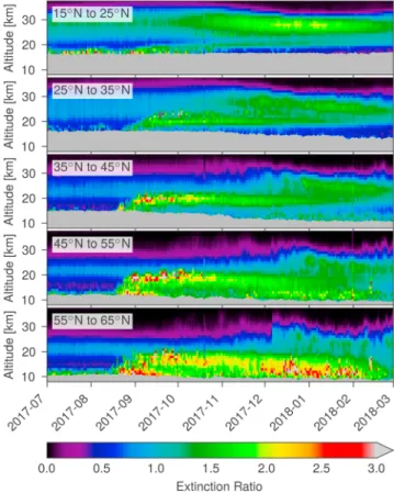
The daily zonal average time series of OMPS‐LP aerosol extinction ratio, shown in Figure 2 for 10° latitude bands, also clearly shows the sustained impact of the forestfire aerosol in each latitude band near 20‐km altitude from mid‐August until approximately January 2018. From early September between 25° and 45°N, very little change in the altitude of the layer is observed over the 5 months and aerosol levels have effectively decayed to background values by February 2018. Although still higher than before thefire event, the levels are indis-tinguishable from the increase due to tropical transport. At the higher latitudes (45–55°N and 55–65°N), there is a slight drop in the altitude of the layer of approximately 3 km over 5 months, and the vertically thin layer of enhanced aerosol from thefire that reaches the tropics rises by approximately 2 km over several months. This daily time series also shows the transport of aerosol from the tropics as a secondary layer that develops above 25 km in October at 25–35°N and appearing successively later at high latitudes. Although this behavior is not observed to the same extent every year, several other years of OMPS‐LP observations reveal similar transport patterns (e.g., 2014 and 2016, not shown).
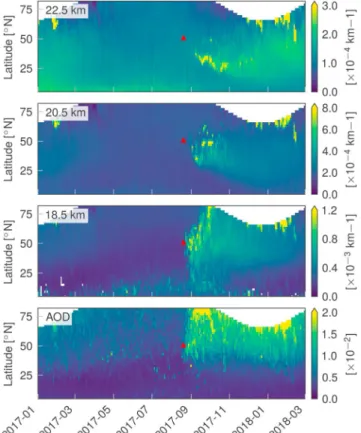
The time series on distinct altitude levels of the OMPS‐LP retrievals, shown in zonal averages in Figure 3, provide another important view of the long‐term transport. The approximate location and time of the forestfire event is marked with a red triangle in each panel. At 17.5 km, the effect of the fires is observed essentially immediately and spreads in latitude both northward and southward but more effectively to the north. At 22.5 km, the aerosol from thefire is not observed until approximately 2 weeks after the fire and appears over 20° of latitude south of thefire location, revealing impressive transport and lofting of the aerosol. The aerosol persists at this level in a fascinatingly coherent plume over more than a month, mean-dering in latitude near the edge of the tropics, before dispersing throughout the Northern Hemisphere. The stratospheric aerosol optical depth (AOD), which is found by integrating the vertical extinction profiles from the tropopause (bottom panel of Figure 3) shows that the vast majority of the total effect is confined to the middle and high latitudes.
Figure 2. Daily time series of zonal average Ozone Mapping and Profiler Suite—Limb Profiler aerosol extinction ratio (aerosol to molecular) at 750 nm for 10° latitude bands from July 2017 to February 2018. Enhanced aerosol extinction from the forestfire is observed in each latitude band near 20‐km altitude from mid‐August until approximately January 2018. Regions below the tropopause are shown as gray.
A detailed comparison of near‐coincident SAGE III/ISS and OMPS‐ LP aerosol extinction profiles during this time period shows many cases where the two instruments report very similar observations, in both profile shape and magnitude. However, there are also many cases where the coincident profiles are substantially different, with varying layer heights and magnitudes. Indeed, it can be a challenge to interpret limb observations in such situations of horizontal variability and strong gradients due to the long line of sight of the observation geometry. Yet the sampling density of the OMPS‐LP observations coupled with the tomographic retrieval provides oppor-tunity to begin to understand these differences. Here, in Figure 4, we show two examples of near coincident OMPS‐LP and SAGE III/ISS observations. Coincidence criteria of 6 hr, 3° latitude, and 20° longitude are used, and often this finds OMPS‐LP measurements from two successive orbits. For each grouping of threefigures, the locations of OMPS‐LP retrievals are shown on the map in red and the tangent point locations of near‐coincident SAGE III/ISS occultation in blue. The aerosol extinction“curtain” produced by the USask 2D retrieval for the OMPS orbit closest to the SAGE III/ISS measurement is shown in the color scale in the top left, with the location of the SAGE III/ISS scan marked with the white line. In the right panels of each grouping, the closest OMPS‐LP and SAGE III/ISS profiles are shown, along with gray shading to indicate the range of values observed by OMPS‐LP across the coincidences. For the case shown in the top grouping from 29 September, the layered vertical structure and magnitudes of the coincident aerosol extinction profiles are very similar in both measurements, and the 2‐D curtain shows relatively slowly varying structure in latitude. Differences in this case could be due to differences in vertical resolution. However, the second case, which shown in the bottom panels, is from 3 days later and shows very different measurements from the coincident OMPS‐LP and SAGE III/ISS profiles. There is a dense, coherent layer very close to the SAGE III/ISS measurement that is not visible in the closest OMPS‐LP measurement but shows up clearly in the 2‐D curtain of successive measurements. The SAGE III/ISS profile shows some evidence of this layer but at a slightly lower altitude due to the fact that it is not sampled directly at the tangent point of the observation. This highlights the utility of the densely sampled limb scatter observations, especially when used in combination with the occultation measurements.
4. Analysis and Discussion
The extent of the observations from these limb observations together with windfields reveals the story of the forestfire aerosol's spatiotemporal evolution during several months that followed the event. Here we choose not to use trajectories, which, unless coupled with a radiative model and aerosol microphysical cycles, cannot be used to account for the plume motion for long.
Figure 5 shows OMPS measurements of elevated aerosol extinction over several months and at distinct altitude levels. In the left column, each dot represents one measurement of elevated aerosol extinction, with the date of the measurement indicated by the color. Panels a, b, and c show the evolution between 15 August and 15 November at altitude levels of 22.5, 20.5, and 18.5 km, respectively. Panel d shows the evolution from 1 November to 31 December, also at 22.5 km. The extinction threshold used to distinguish the plume from background aerosol levels is shown in the bottom left of each panel. In the right column, the National Centers for Environmental Prediction wind vector at the approximate time and location of the elevated aerosol measurements is shown.
Figure 3. Daily time series of zonal average Ozone Mapping and Profiler Suite— Limb Profiler aerosol extinction at three altitude levels and the total
stratospheric aerosol optical depth (AOD). The approximate location and time of the forestfire event is marked with the red triangle. White regions are not sampled by Ozone Mapping and Profiler Suite due to seasonally changing geographic coverage.
Comparison of the panels shows that the movement of elevated aerosol at each level is largely consistent with the windfields. At 18.5 km the plume isfirst detected in August over North America and moves consis-tently to the east skirting the northern edge of the Asian Summer Monsoon Anticyclone, which is still relatively strong at this time in the upper troposphere. The plume then continues moving eastward. More interesting dynamics are observed at the higher altitudes. The aerosol that ascended to 20.5 km above Europe moves southward toward central Asia where it further ascends to 22.5‐km level, probably both diabatically and adiabatically as the isentroposes rise quickly there. By mid‐September the plume at 20.5 km splits in two patches that then depart in the opposite directions. As of this moment, these are essen-tially two independent aerosol plumes with different evolution. The westbound patch continues its further ascent to 22.5 km, gets entrained by tropical easterly winds, and remains within the jet for quite a while. The eastbound patch is displaced to the north and ascends to 22.5 km somewhat slower.
In mid‐November the westbound aerosol gets entrained by an anticyclo-nic pattern above the central Atlantic and is rerouted north and then east. It does not appear that the Asian Summer Monsoon greatly influences the ascent of the aerosol in this case.
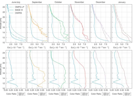
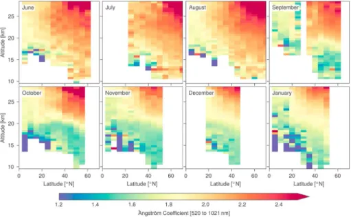
The multispectral aerosol extinction measurements from SAGE III/ISS and the combination of solar occultation and limb scattering observa-tions can provide an indication of changes in aerosol composition and size distribution. Figure 6 shows median 1,020‐ to 525‐nm spectral ratio from SAGE III/ISS in 40–50°N latitude band for each month from July through January. The median profile from July is repeated in each panel to provide a reference for the prefire conditions. This ratio, which is sen-sitive to aerosol size and composition, increases from approximately 0.25 to 0.35 within the enhanced aerosol layer. This increase is also sus-tained over several months and rises slowly with time. Longer wave-length ratios show much smaller changes, with the median 1,550‐ to 1,020‐nm spectral ratio increasing by only 0.02 in the enhanced layer for the months following the fire. Also shown in the top row of Figure 6 is the median extinction at 755 nm for same time periods, including the corresponding OMPS‐LP and OSIRIS median profiles (OSIRIS loses coverage of northern midlatitudes in September). As the aerosols age and the extinction levels decrease, the spectral ratio relaxes slightly toward background levels. However, at high altitudes in December and January the intrusion of aerosol from the tropics also modifies the spectral ratio. Figure 7 plots the zonal, monthly averaged Angstrom exponent, calculated using the same two SAGE III wavelengths, over 8 months starting in June 2017. By September the decrease in Angstrom exponent from the forestfire aerosol in the lower stratosphere north of 40°N is evi-dent, as is the southward transport to the tropics in the following months. As this occurs, the Angstrom exponent does relax slowly to background, but the extinction (see Figure 1) and Angstrom exponent both remain perturbed from background conditions in January. As mentioned above, some of the change at higher latitudes in January, particularly at higher altitudes, is due to intrusions from the tropics. Although a decrease in Angstrom exponent, as observed here, is often interpreted simply as an increase in particle size consistent with the Mie scattering solution for spherical particles, the interpretation is complicated by the inclusion of organics from thefire such as black carbon so we hesitate to speculate on the particle size from these observations.
While there is better than ~20% agreement between occultation and limb scatter measurements of the fire‐generated aerosol layer in Figure 6, this is somewhat unexpected given that the size and composition of the aerosol is very likely quite different than the assumed log‐normal size distribution of spherical
Figure 4. Orbital curtains of aerosol extinction retrieved from OMPS‐LP measurements using the USask tomographic retrieval algorithm (corresponding red points on map) and coincident SAGE III/ISS measurements (corresponding blue points on map). Filled red points indicate an OMPS measurement that falls within the coincidence criteria. SAGE III/ISS measurement tangent altitudes are marked on the OMPS‐LP curtain with a white line. LP = Limb Profiler; OMPS = Ozone Mapping and Profiler Suite; SAGE = Stratospheric Aerosol and Gas Experiment.
Figure 5. Long‐term evolution of enhanced aerosol levels (left panels) along with National Centers for Environmental Prediction windfields (right panels) at three altitude levels. The color of the markers corresponds to the time of the measurement.
Figure 6. Top row: The median 750‐nm aerosol extinction profile in the 40–50°N latitude range measured by SAGE III/ ISS (solid), OSIRIS (short dash), and OMPS (long dash). The median profile measured by SAGE III/ISS in July is included in blue on each successive plot as a reference for the prefire conditions. Bottom row: The median spectral ratio calculated between SAGE III/ISS aerosol extinction at 1,020 to 525 nm shows a change in the enhanced aerosol likely indicating a change in particle size and/or composition. Again, the July profile is repeated in blue for reference on each successive plot. ISS = International Space Station; OMPS‐LP = Ozone Mapping and Profiler Suite—Limb Profiler; OSIRIS = Optical Spectrograph and InfraRed Imaging System; SAGE = Stratospheric Aerosol and Gas Experiment.
hydrated sulfate droplets in the OSIRIS and OMPS‐LP retrieval algorithm. Use of limb scattering measurements in these conditions therefore warrant a brief investigation of possible errors. Estimating the error in the limb scattering retrievals is complicated by the potentially large changes from background conditions. As mentioned previously, the limb scattering measurements are sensitive to microphysical assumptions in the retrieval process. Both retrievals assume a sulfuric acid/water mix with an index of refraction of 1.43 + i3.7 × 10−5. Deviations from the assumed size, as is suggested by the SAGE III particle size retrieval, will increase possible biases. While the relatively forward scattering geometry of the OMPS‐LP measurements limits the impact of these changes, the phase function may still vary by 40% or more in some conditions (see supporting information Figure S1). While changes in the index of refraction were not visible in the SAGE III measurements they may nonetheless be present, and this would also potentially bias the limb scattering measurements. Lidar measurements of the relatively fresh plume in the days and weeks following the Canadian fire indicate single scattering albedos of approximately 0.8 to 0.9 (Haarig et al., 2018; Hu et al., 2019) suggesting some increase in absorbing material. Biases due to the assumed real or imaginary index of refraction were tested using values ranging from 1.43 to 1.34 for the real component and 0.003 to 0.03 for the imaginary component and could also lead to errors of 50% or more (see supporting information Figures S2 and S3). Also, while it is difficult to quantify the sulfate fraction in the presence of smoke particles, the index of refraction does have large error bars depending on the organics and black carbon makeup, with some secondary organic aerosols having index of refraction between 1.4 and 1.6 (Kim et al., 2010) and black/brown carbon higher at 1.7 to 2.0 (Bond & Bergstrom, 2006). It is likely that smoke particles in the plume have a higher real refractive index than sulphates (Fuller et al., 1999; Levin et al., 2010), but how this changes with age is more difficult to estimate. Errors due to underestimation of the real index of refraction have a similar magnitude as overestimation.
Figure 7. Monthly zonal average Angstrom exponent derived from the Stratospheric Aerosol and Gas Experiment III/ International Space Station measurements at 1,020 and 525 nm from June 2017 to January 2018.
Figure 8. The top panel shows the SAGE III 750‐nm extinction ratio in the Northern Hemisphere averaged into 5‐day bins. Below that is the OMPS 750‐nm extinction, also in 5‐day averages for measurements within ±3° latitude of the mean SAGE III measurement for those 5 days. The third panel shows the percent difference between the SAGE III and OMPS time series. Thefinal panel shows the mean SAGE III latitude at each time interval. OMPS = Ozone Mapping and Profiler Suite; SAGE = Stratospheric Aerosol and Gas Experiment.
Although there is the possibility for large errors in the limb scattering retrieval, these errors are difficult to estimate quantitatively as discussed above, and direct comparison with SAGE measurements not affected by these assumptions likely provides a better estimate. Figure 8 shows 5‐ day averaged SAGE III and OMPS extinction measurements within ±3° of the mean SAGE latitude for each time bin. The third panel shows the percent difference between the instruments computed as (SAGE III − OMPS)/SAGE III × 100%. Thefinal panel shows the mean latitude of the SAGE III measurements in each 5‐day period. Errors are generally within approximately 20%. Occasional differences of 50% are seen in the 1‐month period immediately following the fires, although some of this may be due to sampling of the inhomogeneous early plume, as discussed earlier. Overall, this indicates that limb scattering measurements, while imperfect, still provide robust measurements, even in conditions that stray from background assumptions. This makes quantitative comparison of the 2017 fires with previous large fires possible, even during periods where solar occultation measurements are not available.
OSIRIS measurements, which began in 2001, extend stratospheric aerosol measurements to the present day and join the newer OMPS‐LP and SAGE III/ISS measurements to the historical SAGE record (Rieger et al., 2015). Before this 2017 event, the largest impact on stratospheric aerosol levels from a fire in the entire SAGE‐OSIRIS record starting in 1984 was observed in 2009 from an Australian bushfire at 37°S. Figure 9 shows a comparison of the 2017 forestfire event with OMPS‐LP measurements to the 2009 Australian bush fire event in OSIRIS measurements. In each case thefigure shows the difference in monthly zonal average aerosol extinction between the month of and following the event, with the month before the event. Clearly, the 2017 event is substantially larger in magnitude and reaches essentially the same altitude. OSIRIS measurements can saturate at volcanically influenced levels of aerosol (Fromm et al., 2014) but the impact of this effect in the months following the February, 2009, event is negligible due to the relatively lower levels of extinction caused by the wildfire. A direct comparison of the two events with only OSIRIS measurements is not possible due to missing coverage of the Northern Hemisphere in 2017 after September.
5. Summary and Conclusions
Limb sounding satellite observations of stratospheric aerosol extinction following the intense 2017 forestfire events in western North America show that thefire enhanced aerosol levels throughout the Northern Hemisphere for more than 5 months. A sustained layer between approximately 18–22 km reached median values of extinction of almost 10−3km−1, which is approximately an order of magnitude higher than the background levels before thefires. The altitude of the layer did not change substantially over the 5‐month time period, and the higher secondary layer observed at midlatitudes in November and December is due to transport of background aerosol from the tropics. This is by far the largest stratospheric aerosol impact from fire‐generated aerosol measured in the 40‐year record of satellite limb observations from SAGE, OSIRIS, and OMPS‐LP observations.
References
Ansmann, A., Baars, H., Chudnovsky, A., Mattis, I., Veselovskii, I., Haarig, M., et al. (2018). Extreme levels of Canadian wildfire smoke in the stratosphere over central Europe on 21–22 August 2017. Atmospheric Chemistry and Physics, 18, 11,831–11,845. https://doi.org/ 10.5194/acp‐18‐11831‐2018
Bates, D. R. (1984). Rayleigh scattering by air. Planetary and Space Science, 32(6), 785–790.
Acknowledgments
OSIRIS and OMPS‐LP USask 2D Level 2 data are publicly available by request at ftp://odin‐osiris.usask.ca. SAGE III/ISS and OMPS‐LP Level 1b data are publicly available at the NASA Langley Data Center.
Figure 9. (left) The difference in aerosol extinction measured during and after the February 2009 Australian bush fire event measured by OSIRIS (relative to January 2009). (right) The same during and after the August 2017 Canadian forest fire event measured by OMPS (relative to July 2017). The black triangles mark the approximate latitude of the fires. Region below the thermal tropopause is shown in gray. OMPS = Ozone Mapping and Profiler Suite; OSIRIS = Optical Spectrograph and InfraRed Imaging System.
Bond, T. C., & Bergstrom, R. W. (2006). Light absorption by carbonaceous particles: An investigative review. Aerosol Science and Technology, 40(1), 27–67. https://doi.org/10.1080/02786820500421521
Bourassa, A. E., Degenstein, D. A., Elash, B. J., & Llewellyn, E. J. (2010). Evolution of the stratospheric aerosol enhancement following the eruptions of Okmok and Kasatochi: Odin‐OSIRIS measurements. Journal of Geophysical Research, 115, D00L03. https://doi.org/10.1029/ 2009JD013274
Bourassa, A. E., Degenstein, D. A., Gattinger, R. L., & Llewellyn, E. J. (2007). Stratospheric aerosol retrieval with optical spectrograph and infrared imaging system limb scatter measurements. Journal of Geophysical Research, 112, D10217. https://doi.org/10.1029/ 2006JD008079
Bourassa, A. E., Degenstein, D. A., & Llewellyn, E. J. (2008). SASKTRAN: A spherical geometry radiative transfer code for efficient esti-mation of limb scattered sunlight. Journal of Quantitative Spectroscopy and Radiative Transfer, 109(1), 52–73.
Bourassa, A. E., Rieger, L. A., Lloyd, N. D., & Degenstein, D. A. (2012). Odin‐OSIRIS stratospheric aerosol data product and SAGE III intercomparison. Atmospheric Chemistry and Physics, 12(1), 605–614. https://doi.org/10.5194/acp‐12‐605‐2012
Damadeo, R. P., Zawodny, J. M., Thomason, L. W., & Iyer, N. (2013). SAGE version 7.0 algorithm: Application to SAGE II. Atmospheric Measurement Techniques, 6(12), 3539–3561. https://doi.org/10.5194/amt‐6‐3539‐2013
Fromm, M., Bevilacqua, R., Servranckx, R., Rosen, J., Thayer, J. P., Herman, J., & Larko, D. (2005). Pyro‐cumulonimbus injection of smoke to the stratosphere: Observations and impact of a super blowup in northwestern Canada on 3–4 August 1998. Journal of Geophysical Research, 110, D08205. https://doi.org/10.1029/2004JD005350
Fromm, M., Kablick, G. III, Nedoluha, G., Carboni, E., Grainger, R., Campbell, J., & Lewis, J. (2014). Correcting the record of volcanic stratospheric aerosol impact: Nabro and Sarychev Peak. Journal of Geophysical Research: Atmospheres, 119, 10–343.
Fuller, K. A., Malm, W. C., & Kreidenweis, S. M. (1999). Effects of mixing on extinction by carbonaceous particles. Journal of Geophysical Research, 104(D13), 15,941–15,954. https://doi.org/10.1029/1998JD100069
Fyfe, J. C., Salzen, K. V., Cole, J. N. S., Gillett, N. P., & Vernier, J. P. (2013). Surface response to stratospheric aerosol changes in a coupled atmosphere–ocean model. Geophysical Research Letters, 40, 584–588. https://doi.org/10.1002/grl.50156
Haarig, M., Ansmann, A., Baars, H., Jimenez, C., Veselovskii, I., Engelmann, R., & Althausen, D. (2018). Depolarization and lidar ratios at 355, 532, and 1064 nm and microphysical properties of aged tropospheric and stratospheric Canadian wildfire smoke. Atmospheric Chemistry and Physics, 18(16), 11,847–11,861. https://doi.org/10.5194/acp‐18‐11847‐2018
Hu, Q., Goloub, P., Veselovskii, I., Bravo‐Aranda, J.‐A., Popovici, I. E., Podvin, T., et al. (2019). Long‐range‐transported Canadian smoke plumes in the lower stratosphere over northern France. Atmospheric Chemistry and Physics, 19(2), 1173–1193. https://doi.org/10.5194/ acp‐19‐1173‐2019
Kent, G. S., & McCormick, M. P. (1984). SAGE and SAM II measurements of global stratospheric aerosol optical depth and mass loading. Journal of Geophysical Research, 89(D4), 5303–5314. https://doi.org/10.1029/JD089iD04p05303
Khaykin, S. M., Godin‐Beekmann, S., Hauchecorne, A., Pelon, J., Ravetta, F., & Keckhut, P. (2018). Stratospheric smoke with unprece-dentedly high backscatter observed by lidars above southern France. Geophysical Research Letters, 45, 1639–1646. https://doi.org/ 10.1002/, https://doi.org/10.1002/2017GL076763
Kim, H., Barkey, B., & Paulson, S. E. (2010). Real refractive indices ofα‐and β‐pinene and toluene secondary organic aerosols generated from ozonolysis and photo‐oxidation. Journal of Geophysical Research, 115, D24212. https://doi.org/10.1029/2010JD014549 Kremser, S., Thomason, L. W., von Hobe, M., Hermann, M., Deshler, T., Timmreck, C., et al. (2016). Stratospheric aerosol—Observations,
processes, and impact on climate. Reviews of Geophysics, 54, 278–335. https://doi.org/10.1002/2015RG000511
Laat, A. T. J., Stein Zweers, D. C., & Boers, R. (2012). A solar escalator: Observational evidence of the self‐lifting of smoke and aerosols by absorption of solar radiation in the February 2009 Australian Black Saturday plume. Journal of Geophysical Research, 117, D04204. https://doi.org/10.1029/2011JD017016
Levin, E. J. T., McMeeking, G. R., Carrico, C. M., Mack, L. E., Kreidenweis, S. M., Wold, C. E., et al. (2010). Biomass burning smoke aerosol properties measured during Fire Laboratory at Missoula Experiments (FLAME). Journal of Geophysical Research, 115, D18210. https:// doi.org/10.1029/2009JD013601
Rieger, L. A., Bourassa, A. E., & Degenstein, D. A. (2015). Merging the OSIRIS and SAGE II stratospheric aerosol records. Journal of Geophysical Research: Atmospheres, 120, 8890–8904. https://doi.org/10.1002/2015JD023133
Rieger, L. A., Malinina, E. P., Rozanov, A. V., Burrows, J. P., Bourassa, A. E., & Degenstein, D. A. (2018). A study of the approaches used to retrieve aerosol extinction, as applied to limb observations made by OSIRIS and SCIAMACHY. Atmospheric Measurement Techniques, 11(6), 3433–3445. https://doi.org/10.5194/amt‐11‐3433‐2018
Robock, A. (2000). Volcanic eruptions and climate. Reviews of Geophysics, 38(2), 191–219. https://doi.org/10.1029/1998RG000054 Seftor, C. (2017). Record breaking aerosol index values over Canada, NASA OMPS blog. Retrieved from https://ozoneaq.gsfc.nasa.gov/
omps/blog/2017/08/record‐breaking‐aerosol‐index‐value‐over‐canada, Accessed May 15.
Solomon, S., Daniel, J. S., Neely, R. R., Vernier, J. P., Dutton, E. G., & Thomason, L. W. (2011). The persistently variable“background” stratospheric aerosol layer and global climate change. Science, 333(6044), 866–870. https://doi.org/10.1126/science.1206027 Thomason, L. W., Moore, J. R., Pitts, M. C., Zawodny, J. M., & Chiou, E. W. (2010). An evaluation of the SAGE III version 4 aerosol
extinction coefficient and water vapor data products. Atmospheric Chemistry and Physics, 10(5), 2159–2173. https://doi.org/10.5194/acp‐ 10‐2159‐2010
Trepte, C. R., & Hitchman, M. H. (1992). Tropical stratospheric circulation deduced from satellite aerosol data. Nature, 355(6361), 626–628. https://doi.org/10.1038/355626a0
Vernier, J. P., Thomason, L. W., Pommereau, J. P., Bourassa, A., Pelon, J., Garnier, A., et al. (2011). Major influence of tropical volcanic eruptions on the stratospheric aerosol layer during the last decade. Geophysical Research Letters, 38, L12807. https://doi.org/10.1029/ 2011GL047563
Zawada, D. J., Dueck, S. R., Rieger, L. A., Bourassa, A. E., Lloyd, N. D., & Degenstein, D. A. (2015). High‐resolution and Monte Carlo additions to the SASKTRAN radiative transfer model. Atmospheric Measurement Techniques, 8(6), 2609–2623.
Zawada, D. J., Rieger, L. A., Bourassa, A. E., & Degenstein, D. A. (2018). Tomographic retrievals of ozone with the OMPS Limb Profiler: Algorithm description and preliminary results. Atmospheric Measurement Techniques, 11(4), 2375–2393. https://doi.org/10.5194/amt‐ 11‐2375‐2018
Erratum
In the originally published version of this article, a typesetting error switched the captions of Figures 8 and 9. The figure captions have since been corrected, and this version may be considered the autho-ritative version of record.