HAL Id: hal-00295719
https://hal.archives-ouvertes.fr/hal-00295719
Submitted on 11 Aug 2005
HAL is a multi-disciplinary open access
archive for the deposit and dissemination of
sci-entific research documents, whether they are
pub-lished or not. The documents may come from
teaching and research institutions in France or
abroad, or from public or private research centers.
L’archive ouverte pluridisciplinaire HAL, est
destinée au dépôt et à la diffusion de documents
scientifiques de niveau recherche, publiés ou non,
émanant des établissements d’enseignement et de
recherche français ou étrangers, des laboratoires
publics ou privés.
simulation with a chemistry-climate model employing
realistic forcing
M. Dameris, V. Grewe, M. Ponater, R. Deckert, V. Eyring, F. Mager, S.
Matthes, C. Schnadt, A. Stenke, B. Steil, et al.
To cite this version:
M. Dameris, V. Grewe, M. Ponater, R. Deckert, V. Eyring, et al.. Long-term changes and variability
in a transient simulation with a chemistry-climate model employing realistic forcing. Atmospheric
Chemistry and Physics, European Geosciences Union, 2005, 5 (8), pp.2121-2145. �hal-00295719�
www.atmos-chem-phys.org/acp/5/2121/ SRef-ID: 1680-7324/acp/2005-5-2121 European Geosciences Union
Chemistry
and Physics
Long-term changes and variability in a transient simulation with a
chemistry-climate model employing realistic forcing
M. Dameris1, V. Grewe1, M. Ponater1, R. Deckert1, V. Eyring1, F. Mager1,*, S. Matthes1, C. Schnadt1,**, A. Stenke1,
B. Steil2, C. Br ¨uhl2, and M. A. Giorgetta3
1Institut f¨ur Physik der Atmosph¨are, DLR-Oberpfaffenhofen, Wessling, Germany 2Max-Planck-Institut f¨ur Chemie, Mainz, Germany
3Max-Planck-Institut f¨ur Meteorologie, Hamburg, Germany
*now at: University of Cambridge, Centre for Atmospheric Science, Department of Geography, Cambridge, UK **now at: ETH Z¨urich, Institut f¨ur Atmosph¨are und Klima, Z¨urich, Switzerland
Received: 25 January 2005 – Published in Atmos. Chem. Phys. Discuss.: 14 April 2005 Revised: 29 June 2005 – Accepted: 1 August 2005 – Published: 11 August 2005
Abstract. A transient simulation with the interactively
cou-pled chemistry-climate model (CCM) E39/C has been car-ried out which covers the 40-year period between 1960 and 1999. Forcing of natural and anthropogenic origin is pre-scribed where the characteristics are sufficiently well known and the typical timescales are slow compared to synoptic timescale so that the simulated atmospheric chemistry and climate evolve under a “slowly” varying external forcing. Based on observations, sea surface temperature (SST) and ice cover are prescribed. The increase of greenhouse gas and chlorofluorocarbon concentrations, as well as nitrogen oxide emissions are taken into account. The 11-year solar cycle is considered in the calculation of heating rates and photoly-sis of chemical species. The three major volcanic eruptions during that time (Agung, 1963; El Chichon, 1982; Pinatubo, 1991) are considered. The quasi-biennial oscillation (QBO) is forced by linear relaxation, also known as nudging, of the equatorial zonal wind in the lower stratosphere towards ob-served zonal wind profiles. Beyond a reasonable reproduc-tion of mean parameters and long-term variability character-istics there are many apparent features of episodic similari-ties between simulation and observation: In the years 1986 and 1988 the Antarctic ozone holes are smaller than in the other years of that decade. In mid-latitudes of the South-ern Hemisphere ozone anomalies resemble the correspond-ing observations, especially in 1985, 1989, 1991/1992, and 1996. In the Northern Hemisphere, the episode between the late 1980s and the first half of the 1990s is dynami-cally quiet, in particular, no stratospheric warming is found between 1988 and 1993. As observed, volcanic eruptions strongly influence dynamics and chemistry, though only for
Correspondence to: M. Dameris
few years. Obviously, planetary wave activity is strongly driven by the prescribed SST and modulated by the QBO. Preliminary evidence of realistic cause and effect relation-ships strongly suggests that detailed process-oriented studies will be a worthwhile endeavour.
1 Introduction
In recent years, more and more results of interactively cou-pled chemistry-climate models (CCMs) have become avail-able (e.g. Rozanov et al., 2001; Austin, 2002; Nagashima et al., 2002; Pitari et al., 2002; Schnadt et al., 2002; Steil et al., 2003; Manzini et al., 2003). First of all, they have been developed to examine the feedback between dynami-cal, physidynami-cal, and chemical processes in the atmosphere, with a particular focus on the upper troposphere and stratosphere. The primary purpose of CCMs is to support analyses of long-term observations and to explain recent changes and variabil-ity of chemical composition and dynamics. Like other com-plex model systems, CCMs must be carefully checked with respect to their abilities and deficiencies to describe present and recent atmospheric conditions before they can be applied for reliable estimates of future changes (e.g. Eyring et al., 2005b).
Currently, there are two concepts to perform numerical ex-periments with CCMs: Firstly, so-called time-slice experi-ments are well suited to investigate the internal variability of the coupled chemistry-climate system and to indicate and es-timate the significance of specific changes of certain parame-ters or processes in past, present or future climate states with respect to a reference state. Such simulations are carried out with fixed boundary conditions given for a specific year, for
example, concentrations of greenhouse gases (GHGs), emis-sions of natural and anthropogenic source gases, sea surface temperatures (SSTs), etc., to investigate the corresponding “equilibrium climate”. The comparison of time-slice simu-lations among each other is favourable to identify and inter-pret long-term temporal developments, e.g., pattern changes, in case that the assessment of statistical significance poses a problem. Secondly, results derived from transient model sim-ulations, which consider observed gradual changes in GHGs and other boundary conditions, allow a more straightforward comparison with the actual temporal development of the real atmosphere. In particular, non-persistent perturbations of the stationary or slowly varying behaviour of the real atmosphere can be included in the simulation for a more detailed model evaluation. Both modelling strategies lead to useful results for a better understanding of atmospheric processes. This is demonstrated by a considerable number of papers which have recently been published (e.g. Rozanov et al., 2001; Austin, 2002; Nagashima et al., 2002; Pitari et al., 2002; Schnadt et al., 2002; Steil et al., 2003; Manzini et al., 2003). A number of examples concerning strengths and weaknesses of CCMs were discussed in Austin et al. (2003) where the results of different CCMs have been compared with obser-vations and each other. The studies mentioned above have concentrated on the stratosphere, others have the main fo-cus on the troposphere (e.g. Wang and Prinn, 1999; Johnson et al., 1999; Grewe et al., 2001a). All these CCM studies have in common that they focus on specific cause and ef-fect relationships with respect to atmospheric chemistry and dynamics, but rarely have tried to investigate the complete system.
It is the central objective of this paper to investigate and discuss the results of a transient simulation with a state-of-the-art CCM. While E39/C simulates tropospheric and lower stratospheric processes as components of equal importance, the focus of our analysis is on the upper troposphere and lower stratosphere. Although E39/C extends only to about 30 km and therefore neglects direct influences of the up-per stratosphere, we do not believe that this has a signifi-cant impact on our conclusions. Possible boundary effects are discussed if appropriate. Moreover, we have tried to in-clude a comprehensive set of external forcings on variability and trends in order to allow a fair comparison with observa-tions and to assess the capability to reproduce the develop-ment of the real atmosphere. To our knowledge, this is one of the first transient CCM simulations which, beyond trends in trace gas emissions and concentrations, also considers the forcings from observed sea surface temperature (SST) vari-ability, from large volcanic eruptions, the 11-year solar cy-cle effect, and the quasi-biennial oscillation (QBO). They all have significant impacts on processes which determine dy-namics and chemistry of the atmosphere. This investigation aims to identify and better understand the importance of ex-ternal forcings on climate and chemical composition. A key question is how deterministic the response of a non-linear
model system to such forcings is. However, it is impossible to give a reliable and final answer to this question in a sin-gle paper. The employed experimental setup using observed SSTs without additional sensitivity simulations does not al-low to determine to what extent the SST development over recent decades is a deterministic response to external forcing and to what extent it resulted from internal variability. This would require at least ensemble simulations with E39/C to reduce the level of stochastic variability, while use of a cou-pled interactive ocean would be even more favourable. Nev-ertheless, a detailed comparison of model results and data products derived from long-term observations is presented to advance our understanding of the model’s potential and to approach a quantitative answer to this question.
In the following section a brief description of the model and the experimental set-up is given. Section 3 concentrates on long-term changes (trends) in observations and model data. The response due to prescribed forcings (i.e., volcanic eruptions, QBO, solar cycle, SSTs) is discussed in Sect. 4. The results discussed in this paper concentrate on the upper troposphere and lower stratosphere region (UTLS), which is conditioned by the model domain. The last section gives a brief outlook.
2 Model description and experimental set up
2.1 The CCM ECHAM4.L39(DLR)/CHEM
In this study, the interactively coupled CCM ECHAM4.L39(DLR)/CHEM (hereafter: E39/C) is used for a transient model simulation covering the time period from 1960 to 1999. Previously, the model system has been applied for several investigations, but results from time-slice runs were used exclusively. A basic description of E39/C is given in detail by Hein et al. (2001), Grewe et al. (2001b), and Schnadt et al. (2002). In the following, the setup of E39/C is only briefly summarised.
The horizontal resolution of E39/C is spectral T30, i.e., dynamical processes have an isotropic resolution of about 670 km. The corresponding Gaussian transform latitude-longitude grid, on which the model physics, chemistry, and tracer transport are calculated, has a mesh size of 3.75◦×3.75◦. In the vertical, E39/C has 39 layers from the surface up to the top layer centred at 10 hPa (Land et al., 2002). The chemistry model CHEM (Steil et al., 1998) is based on a generalised family concept which has three up-grades (Steil et al., 2003): a) reduce the use of the steady state approximation; b) consider coupling between families by solving combined families; and c) definitions of fami-lies for transport and chemistry are different. CHEM ac-counts for relevant stratospheric and tropospheric O3related
homogeneous chemical reactions and heterogeneous chem-istry on PSCs and sulphate aerosols. It does not include bromine chemistry. This should influence calculated ozone
Table 1. Overview of the external forces included in the transient model simulation.
Forcing Circulation Chemistry
SST Real observations - GISS/Hadley –
Volcanoes Simulated heating rates Observed/estimated SADs from SAGE
QBO Zonal stratospheric tropical winds –
’nudged’ towards observations
Solar Cycle Changes in the solar constant Changes in extra-terrestrial fluxes (7 bands)
affecting photolysis rates
CO2 Greenhouse gas –
CH4, N2O, CFCS Greenhouse gases Reaction with OH/photolysis impacts strat.
and trop. chemistry
NOxemissions – Impact on ozone chemistry
depletion rates, especially in the Northern Hemisphere, since there ozone is only partly destroyed by chlorine. This has to be taken into account when analysing the model results. The model version used in the present study includes updates of the rate coefficients of gas-phase reactions following JPL (2000). Compared to previous model versions, two hetero-geneous reactions on stratospheric aerosol have been added (ClONO2+HCl→Cl2+HNO3 and HOCl+HCl→Cl2+H2O).
The transport of chlorine components has been improved by transporting both, total chlorine and the partitioning of chlorine species, to minimise numerical diffusion in regions with lower vertical resolution. As a reminder, this model version does not include complex non-methane hydrocarbon (NMHC) chemistry. It only considers intermediate products of the methane oxidation (CH2O, CH3O, CH3O2, and the
HOx-family), which are computed at each time-step. The
photolysis at solar zenith angles (SZAs) larger than 87.5◦ has been implemented into E39/C to account for the effects of twilight stratospheric ozone chemistry. Lamago et al. (2003) showed that modelled temperature as well as ozone fields, particularly in polar regions, improve when SZAs up to 93◦ are considered. Net heating rates and
photoly-sis rates in E39/C are calculated from the current modeled three-dimensional (3-D) distributions of the radiatively ac-tive gases O3, CH4, N2O, H2O, and CFCs, and the 3-D cloud
distribution. The model climatology has been extensively validated; specifically, analyses on the model’s performance in the Arctic stratosphere have been carried out (Hein et al., 2001; Austin et al., 2003).
The parameterisation by Price and Rind (1992) used in previous E39/C simulations to account for NOx emissions
from lightning has been replaced by an improved parameter-isation developed by Grewe et al. (2001b). Grewe et al. re-late the flash rate to the vertical air mass exchange within a convective cloud. A comparison of flash frequencies calcu-lated by E39/C and those derived from the Optical Transient Detector (OTD) observations onboard the MicroLab satellite showed a qualitatively and quantitatively reasonable
agree-ment (Kurz and Grewe, 2002). The parameterisation takes into account intra-cloud and cloud to ground lightning (Price and Rind, 1993) and uses effective NOx emission profiles
(Pickering et al., 1998). The annual mean emission rate over the 40-year simulation period amounts to 5.16 Tg(N)/a. 2.2 Design of the transient simulation
The transient integration of E39/C is designed to represent the atmospheric development during the period from 1960 to 1999. A spin-up of ten years with stationary conditions of the late 1950s precedes the actual transient part of the exper-iment. The simulation aims at reproducing the effect of nat-ural as well as anthropogenic forcings. Natnat-ural factors con-sidered are the 11-year solar cycle, the QBO, and chemical and direct radiative effects of the major volcanic eruptions of Agung in 1963, El Chichon in 1982, and Mt. Pinatubo in 1991. The anthropogenic influence is represented by atmospheric concentrations of the most important GHGs, chlorofluorocarbons (CFCs), and nitrogen oxide emissions. Other ozone precursors in the troposphere are not considered. Carbon monoxide (CO) mixing ratios at the Earth surface are prescribed as a function of latitude and season (Hein et al., 1997) and are kept constant throughout this simulation. Ta-ble 1 gives an overview of the boundary conditions for the transient simulation.
We emphasize that a considerable part of the anthro-pogenic impact on tropospheric climate is accounted for by using a SST development prescribed from observations. The SSTs are given as monthly mean values following the global sea ice and sea surface temperature (HadISST1) data set pro-vided by the UK Met Office Hadley Centre (Rayner et al., 2003). The data are based on blended satellite and in situ observations. For the simulation, a linear interpolation based on the monthly mean values is applied. A few gaps in sea ice coverage appeared which were caused by the interpolation of the original data set to the model grid, e.g., a grid box in the Arctic region which is free of ice is surrounded by grid
Table 2. Total intensity (solar constant, in W/m2) and extra-terrestrial fluxes (in phot/cm2s) at the uppermost model level, as assumed in E39/C. The spectral intervals are given in nm. The val-ues for solar maximum represent valval-ues measured in the year 1991.
value in value in difference
solar minimum solar maximum [in %]
total intensity [W/m2] 1365.00 1366.09 0.1
extra-terrestrial flux at 10 hPa [phot/cm2s]
178.8–202.0 8.7990×10¹² 9.6701×10¹² 9.9 202.0–241.0 1.7007×10¹⁴ 1.7704×10¹⁴ 4.1 241.0–289.9 1.1179×10¹⁵ 1.1396×10¹⁵ 1.9 289.9–305.5 1.2734×10¹⁵ 1.2786×10¹⁵ 0.4 305.5–313.5 7.9740×10¹⁴ 8.0102×10¹⁴ 0.5 313.5–337.5 3.3641×10¹⁴ 3.3660×10¹⁴ 0.1 337.5–422.5 2.0640×10¹⁶ 2.0668×10¹⁶ 0.1 422.5–752.5 1.2865×10¹⁷ 1.2865×10¹⁷ 0.0
boxes which all contain ice. These obvious inconsistencies have been removed by hand.
Both, chemical and direct radiative effects of enhanced stratospheric aerosol abundance from large volcanic erup-tions are considered. For the heterogeneous reacerup-tions cov-ered in the chemistry module, sulphate aerosol surface area densities partly had to be approximated from observations as follows: The original data set consists of monthly and zon-ally averaged sulphate aerosol surface area densities (WMO, 2003). It was deduced from satellite-based extinction mea-surements (SAGE I, SAGE II, SAM II, and SME), as has been described in Jackman et al. (1996), using the method-ology of Rosenfield et al. (1997). The Agung eruption in 1963 is not covered by this data set. As a remedy, the well-documented years following the eruption of Mt. Pinatubo (1991–1994) have been adopted and associated with the pe-riod 1963–1966 with modifications based on published re-sults to account for differences in total mass of sulphate aerosols in the stratosphere, in maximum height of the erup-tion plumes, and in the volcanoes’ geographical locaerup-tion (e.g. Sato et al., 1993; Andronova et al., 1999; Robock, 2000). Above the maximum vertical extent of Agung’s erup-tion plume the annual mean of 1979 has been incorporated. By 1979 the total mass of stratospheric sulphate aerosol had probably returned to its background value, being main-tained by a permanent supply of tropospheric sulphur species (Junge et al., 1961; Mc Cormick et al., 1995). For the time periods 1960–1962 and 1968–1978 the annual mean of 1979 has been adopted, and for the period 1996–1999 the annual mean of 1995 has been used. Additionally, the data set has been interpolated linearly from 177 to 16 vertical levels and from 18 latitudes to 48 latitudes.
Eruption-related radiative heating is implemented in E39/C using pre-calculated monthly and zonal mean net heating rates. These rates are taken from a previous ECHAM4(T42)/L19 (L19 = 19 vertical layers) Pinatubo sen-sitivity experiment, which was forced by a realistic space-time dependent aerosol distribution (Kirchner et al., 1999). Kirchner and colleagues forced their model by aerosol dis-tributions and spectral radiative characteristics calculated applying SAGE II extinctions (same as mentioned above) and used effective radii retrieved by the Upper Atmosphere Research Satellite (UARS). We decided to use the pre-calculated heating rates after interpolating to the 39 layers of E39/C, as no significant difference was expected from a di-rect calculation in E39/C with both ECHAM4 versions using identical radiation codes. The data set provided by Kirchner et al. extends from July 1991 to April 1993. Thus, only part of the eruption-influenced time span was available, e.g., June 1991 (month of eruption) is missed. Therefore, for June 1991 the radiative forcing has been taken as 0.5×July 1991 values, and an exponential decay has been adopted in the period from May 1993 to July 1993. With regard to Agung and El Chi-chon, similar estimates of additional heating rates were not available due to the lack of solicited information of aerosol parameters. Considering the limited information about the pre-Pinatubo eruptions (see above) and as there are strong hints for similar temperature responses in the stratosphere (e.g. Labitzke, 1994), sets of heating rates for the Agung and El Chichon periods have been created with slight modifica-tions to the horizontal structure of the radiative heating dis-tributions. This approach is certainly a simplified one, but due to the lack of consistent information for the three vol-canic eruptions this strategy seems to be reasonable as a first attempt.
The QBO is described based on zonal wind profiles mea-sured near the equator. Radiosonde data from Canton Is-land (1953–1967), Gan/Maledives (1967–1975) and Singa-pore (1976–2000) have been used to develop a time series of monthly mean zonal winds at the equator (Naujokat, 1986; Labitzke et al., 2002). This data set covers the lower strato-sphere up to 10 hPa. It is used to assimilate the QBO in E39/C, such that the QBO is synchronised with other ex-ternal inter-annual variations prescribed in this experiment. For the assimilation it is assumed that the QBO is zonally symmetric, i.e., has little variation along a latitude band, and that it has a Gausian half width of about 12 degree latitude around the equator. The QBO is forced in E39/C by a lin-ear relaxation of the predicted zonal wind towards the con-structed QBO time series, which follows the observed zonal wind profile (Giorgetta and Bengtsson, 1999). This assimila-tion is applied equatorwards of 20◦latitude from 90 hPa up to the highest layer of the model centred at 10 hPa. The re-laxation time scale has been set to 7 days within the QBO core domain. Outside of this core domain the time scale depends on latitude and pressure (Giorgetta and Bengtsson, 1999). Figure 1 shows the results of the assimilated monthly
-20 -20 -20 -20-15 -15 -15 -15 -15 -10 -10 -10 -10 -10 -10 -10 -10 -5 -5 -5 -5 -5 -5 -5 -5 -5 5 5 5 5 5 5 5 5 5 5 5 5 5 5 5 5 5 5 5 5 5 5 5 5 5 5 5 5 5 5 5 5 10 10 10 10 10 10 10 10 Pressure [hPa] 120 144 168 192 216 240 264 288 312 336 360 1960 1962 1964 1966 1968 1970 1972 1974 1976 1978 1980 10 20 50 100 200 400 650 1000 -20 -20 -15 -15 -15 -15 -15 -15 -15 -15 -10 -10 -10 -10 -10 -10 -10 -10 -5 -5 -5 -5 -5 -5 -5 -5 5 5 5 5 5 5 5 5 5 5 5 5 5 5 5 5 5 5 5 5 5 5 5 5 5 5 5 5 5 5 5 5 5 5 5 5 10 10 10 10 10 10 10 10 10 10 Pressure [hPa] 360 384 408 432 456 480 504 528 552 576 600 1980 1982 1984 1986 1988 1990 1992 1994 1996 1998 2000 10 20 50 100 200 400 650 1000 -40 -35 -30 -25 -20 -15 -10 -5 5 10 15 20 [m/s]
Fig. 1. Monthly mean zonal winds (in m/s) near the equator (zonal mean values) in the E39/C model simulation. Negative (positive) wind
speed indicates easterly (westerly) wind.
mean zonal winds of the E39/C run for the time period 1960 to 1999. The assimilated QBO compares well with the ob-served phase state and the obob-served amplitudes of the west-erlies and eastwest-erlies (Giorgetta and Bengtsson, 1999, their Fig. 1).
The influence of the 11-year solar cycle on photolysis rates is parameterised according to the intensity of the 10.7 cm ra-diation of the sun (data available at: http://www.drao.nrc. ca/icarus/www/daily.html). Table 2 gives the values of the extra-terrestrial fluxes in different spectral intervals assumed for high (i.e., these values represent the year 1991) and low solar activity used at the upper boundary of E39/C. The 1991 solar maximum values are employed as reference values for the calculation of respective values for maximum solar activ-ity of the other solar cycles which are considered in the tran-sient run, i.e., 1958, 1969, and 1980. These values are scaled with the intensity of the 10.7 cm flux of the corresponding years. Photolysis rates are calculated in 8 spectral intervals (Landgraf and Crutzen, 1998). The spectral distribution of changes in extra-terrestrial flux is based on investigations presented by Lean et al. (1997). The ozone columns above the model top (centred at 10 hPa) are considered by a sea-sonally dependent climatology which is taken from HALOE observations. It must be mentioned that those climatological
values represent an average of 6 years only and therefore do not consider changes due to the solar cycle. The impact of solar activity changes on short-wave radiative heating rates is prescribed based on changes of the solar constant (see Ta-ble 2). Short-wave radiative heating rates are considered in two spectral intervals (Morcrette, 1999; Fouquart and Bon-nel, 1980), respecting continuum scattering, grey absorption, water vapour and uniformly mixed gases transmission func-tions and ozone transmission.
Continuously changing mixing ratios of the most relevant greenhouse gases (CO2, N2O, CH4) are prescribed, CO2for
the entire model domain, the others at the Earth’s surface ac-cording to Hein et al. (1997) and IPCC (2001; see Fig. 2). As mentioned above, for CO no long-term change is assumed. Changes in hydrocarbons are also not considered, except for methane. Neglecting these species and associated trends may lead to some underestimation of tropospheric ozone changes and an overestimate of OH values, but this should not af-fect significantly our conclusions of this paper. Natural and anthropogenic nitrogen oxide (NOx=NO+NO2) emissions at
the Earth’s surface, and NOx emission from lightning and
air traffic are considered. In the following a brief summary of the individual NOx emission sources and their temporal
Fig. 2. Changes of mixing ratios of CO2(in ppmv), N2O (in ppbv), CH4(in ppmv), and Cly(in ppbv), as adopted in the transient
sim-ulation with E39/C.
The horizontal distribution of NOxemissions from
indus-try is based on Benkovitz et al. (1996). Its temporal develop-ment has been adapted to match the Benkovitz et al. (1996), Hein et al. (2001), as well as the IPCC (2001) values. The in-crease of the emission rates from 1960 to 1999 are assumed to be piecewise constant, i.e., 2.5%/year between 1960 and 1979, 1.5%/year between 1980 and 1989, and 3.9%/year be-tween 1990 and 1999. This should represent the slowdown of emissions during the 1980s in Europe and the stronger increase during the 1990s mainly in Asia. The same geo-graphic distribution is used for all years of the simulation with the global IPCC trend imposed. The different devel-opment in different global regions is neglected because reli-able numbers were not accessible when the model run was started. This is certainly a constraint but should not have a substantial influence on the results discussed in this paper. Anthropogenic NOx emissions include those from surface
transportation as an individual component (Matthes, 2003), which contributes approximately 30% to the total industry emissions (see also Matthes et al., 20051). Ship emissions have been removed from the global dataset (Benkovitz et al., 1996). Instead, a more sophisticated ship emission inven-tory with 1993 annual global NOxemissions of 3.08 Tg(N)
is used as the basic data set (Corbett et al., 1999). Trend estimates of NOxemissions from international shipping for
the time period 1960 to 2000 have been adopted from Eyring et al. (2005a). Based on these assumptions, the annual global NOxemissions from ships for the years 1960 to 1999 amount
to 1.17 Tg(N) and 3.28 Tg(N), respectively. Aircraft NOx
emissions are based on a data set representing 1992 (Schmitt and Brunner, 1997). Trends previous to 1992 have been
ex-1Matthes, S., Grewe, V., Sausen, R., and Roelofs, G.-J.: Global impact of road traffic emissions on the chemical composition of the atmosphere, Atmos. Chem. Phys. Disscuss., submitted, 2005.
trapolated using IPCC (1999). For the period 1992 to 1999 an exponential interpolation has been applied. The aircraft NOx
emissions for the years 1960 to 1999 amount to 0.10 Tg(N) and 0.71 Tg(N), respectively.
Nitrogen oxide emissions from biomass burning are based on Hao et al. (1990) and have been revised using ATSR fire counts (David Lee, pers. comm., 2004). The trend rates used are based on estimates presented in Chapter 4 of IPCC (1999): An increase of NOx emissions from biomass
burn-ing of 7% has been specified for the years between 1992 and 2015 which results in a rate of approximately 0.3%/year. This rate is used in the E39/C transient simulation and it leads to an increase of 13% between 1960 and 1999. Global NOx
soil emissions by micro-biological production are assumed to be constant over the four decades of the transient simu-lation. They are taken from Yienger and Levy (1995). As mentioned above, lightning NOxemissions are calculated
in-teractively, based on the parameterised mean mass flux in the updraft of deep convective clouds (see previous section), re-sulting in a mean annual emission of 5.16 Tg(N). The inter-annual variability ranges between 4.81 and 5.42 Tg(N)/a and the seasonal cycle varies with ±14%. We anticipate that no systematic trend of lightning NOx emissions is found over
the 40-year transient simulation.
To take into account exchange processes from the upper stratosphere, upper boundary conditions are adopted for the two families ClX and NOy at 10 hPa
(ClX=HCl+ClONO2+ClOx,
ClOx=Cl+ClO+ClOH+2·Cl2O2+2·Cl2,
NOy=NOx+N+NO3+2·N2O5+HNO4+HNO3).
They largely determine lower stratospheric nitrogen oxide and chlorine concentrations. Monthly mean concentrations are taken from results of the two-dimensional (2-D) middle atmosphere model by Br¨uhl and Crutzen (1993), which also considers effects of the 11-year solar cycle. For example, the NOy values prescribed at the model’s upper boundary
fluctuate according to solar activity. Since CFCs are not explicitly transported by E39/C, they are included based on results derived from the 2-D model (depending on latitude and altitude), and serve as a source for total chlorine (Cly)
by photolysis within the model domain. The development of CFC concentrations is prescribed in agreement with most recent assumptions (WMO, 2003). Stratospheric Cly has
been calculated as a sum of the simulated ClOx, ClONO2,
HCl fields, and chlorine from the prescribed CFC fields (see Fig. 2). Its temporal evolution reflects the observed development (WMO, 2003, their Figs. 1–7).
3 Long-term trends
In this section climatic variability and trends of key param-eters will be presented and discussed with respect to corre-sponding observations.
Fig. 3. Development of monthly mean total ozone between 1960 and 1999, as calculated with E39/C. The zonal mean values are given in
Dobson Units (DU).
3.1 Ozone
Figure 3 shows the development of monthly and zonal mean total ozone for the whole simulation period. It indicates the well-known features, e.g., highest ozone values in north-ern spring time which is highly variable from year-to-year, low ozone values in the tropics with a small seasonal cy-cle and little interannual variability, a relative ozone max-imum in mid-latitudes of the Southern Hemisphere in late winter/early spring, and a minimum ozone column above the south polar region in the same period. The ozone hole ap-pears for the first time in the year 1982 in E39/C, which is in agreement with observations (Chubachi, 1985; Farman et al., 1985). An additional interesting feature is the absence of to-tal ozone values above 475 DU in the Northern Hemisphere during the late 1980s and the first half of the 1990s. This indicates a period of at least six years without distinct mid-winter warmings of the stratosphere. There is no other com-parable episode in the 40-year simulation. This agrees with the evolution of the real atmosphere, where northern winters from 1989/1990 to 1996/1997 show no major stratospheric warming events (e.g. Naujokat and Pawson, 1996; Naujokat et al., 1997; Pawson and Naujokat, 1999) resulting in sig-nificant springtime ozone losses during these years (e.g. Rex et al., 2004).
For a closer insight into regional and temporal patterns in the interannual variability of ozone changes, Fig. 4 shows total ozone anomalies for the whole model simulation with
respect to mean values based on the years 1964 to 1980. The features discussed above can easily be identified again, es-pecially that ozone depletion begins at high latitudes of the Southern Hemisphere and that the reduction of the ozone layer occurs later in both, the Northern Hemisphere and the tropical region. But there are also some additional eye-catching features: For example, as identified in observations (e.g. Bojkov and Fioletov, 1995), the ozone holes in the years 1986 and 1988 are clearly smaller than in the respective year before. A closer inspection of the dynamics of the polar vor-tices in E39/C during these years indicate in both cases that the vortex is less stable and displaced from the polar region towards lower latitudes, which is very similar to the observed dynamical behaviour of the polar vortices in 1986 and 1988. There are a number of other interesting similarities in mid-latitudes of the Southern Hemisphere, i.e., modelled posi-tive and negaposi-tive ozone anomalies which nicely match ob-servations, in particular in 1985, 1989, 1991, 1992, and 1996 (see Bojkov and Fioletov, 1995, their Plate 1). A process related discussion about possible reasons for these consis-tencies with observations will be given in the next section. Looking into the tropics, there is distinct variability clearly reflecting the QBO signal; this is discussed in more detail in Sect. 4.2.
Before looking more closely at the long-term variability and changes (trends) calculated by the model, we take a look at the systematic bias of total ozone in E39/C. Figures 5a
Fig. 4. Anomalies of total ozone relative to associated mean values derived for the period between 1964 and 1980. Positive (negative) values
(in %) indicate more (less) ozone with regards to the reference period.
and 5b show 20-year mean climatological total ozone val-ues derived from the E39/C simulation, i.e., the 1960s and 1970s, and the 1980s and 1990s. The climatology derived from measurements of the TOMS instrument for the years 1980 to 1999 is displayed in Fig. 5c. A comparison of Figs. 5b and 5c indicates that E39/C is able to reproduce the main features (e.g., regional distribution, seasonal cycle) in qualitative agreement with TOMS observations. In the Northern Hemisphere and the tropics, the model calculates total ozone values which are about 10 to 15% higher than the values derived from TOMS. These model results con-firm the findings of the E39/C time-slice experiments (e.g. Hein et al., 2001). However, in the Southern Hemisphere the model shows an improved behaviour with respect to former studies with E39/C: The absolute total ozone values are in overall agreement with TOMS, merely the ozone hole sea-son in E39/C lasts slightly longer and the mid-latitude ozone maximum is somewhat higher. This model improvement can partly be attributed to the fact that large SZAs are now considered for the calculation of photolysis rates which has a clear impact on the model behaviour, particularly in the Southern Hemisphere (Lamago et al., 2003).
Figure 5d displays the differences between the two E39/C climatologies affected by the ozone hole (1980–1999; Fig. 5b) and the preceding era (1960–1979; Fig. 5a). Since the 1960s and 1970s represent a climatological mean state of an almost unperturbed episode, this climatology can be taken as a basis to derive trends from 1980 onwards. As
an-ticipated, largest changes are found in the south polar region during spring time, where 60 DU less ozone is calculated in the second half of the transient simulation compared with the first half. This amounts to an ozone reduction of about 20% per decade. Especially in the 1990s, ozone decreases steadily with more than 40% less ozone at the end of the century compared to 1980. These estimates agree well with numbers derived from observations. For example, based on TOMS-data for the years between 1978 and 1994, Mc Peters et al. (1996) estimated an ozone loss of 20%/decade.
Also in the Northern Hemisphere, the trend pattern and absolute numbers agree with analyses from measurements: Mc Peters et al. found an ozone reduction in northern spring of about 6%/decade. The model shows a decrease of about 25 DU (Fig. 5d), which relates to a trend of about 5% per decade. A small increase (less than 7 DU) in total ozone is simulated by E39/C in northern summer. It is caused by an increase of tropospheric ozone concentration whereas at the same time no clear change is simulated in the lower strato-sphere (see Fig. 6b). The vertical ozone distribution (Fig. 6a) and its seasonal changes are very similar to results derived from E39/C time-slice experiments (e.g. Hein et al., 2001) which are in reasonable agreement with observations (e.g. Fortuin and Kelder, 1998). The simulated ozone changes throughout the four decades are almost everywhere statisti-cally significant: Ozone mixing ratios have increased dur-ing equinox (MAM, SON) in the middle troposphere of the Northern Hemisphere by more than 10 ppbv, whereas in the
(a) Latitude Time [month] J F M A M J J A S O N D J -90 -60 -30 0 30 60 90 -90 -60 -30 0 30 60 90 175 200 225 250 275 300 325 350 375 400 425 450 475 500 525 550 [DU] (b) Latitude Time [month] J F M A M J J A S O N D J -90 -60 -30 0 30 60 90 -90 -60 -30 0 30 60 90 175 200 225 250 275 300 325 350 375 400 425 450 475 500 525 550 [DU] (c) Latitude Time [month] J F M A M J J A S O N D J -90 -60 -30 0 30 60 90 -90 -60 -30 0 30 60 90 175 200 225 250 275 300 325 350 375 400 425 450 475 500 525 550 [DU] (d) Latitude Time [month] J F M A M J J A S O N D J -90 -60 -30 0 30 60 90 -90 -60 -30 0 30 60 90 -60 -55 -50 -45 -40 -35 -30 -25 -20 -15 -10 -5 0 5 10 [DU]
Fig. 5. Climatologies of total ozone derived from E39/C for the periods 1960 to 1979 (a), 1980 to 1999 (b), and from TOMS measurements
during the years from 1980 to 1999 (c). Differences between the two E39/C climatologies are displayed in (d), where positive (negative) values indicate more (less) ozone in second half of the 40-year transient simulation. Given values are in DU.
lower stratosphere a general decrease is evident, in particular in the polar Southern Hemisphere spring time (SON). The increase of tropospheric ozone mixing ratios is due to the in-creased NOxemissions (e.g. Grewe et al., 2001b) whereas
stratospheric ozone depletion is a consequence of increased halogen loading and temperature decrease in the stratosphere due to an increased abundance of GHGs (e.g. Schnadt et al., 2002).
3.2 Temperature and zonal wind
Climatologies of temperature and zonal mean wind fields for the 1960s and their changes throughout the four decades, as simulated by E39/C, are displayed in Figs. 7 and 8. The mean fields for the 1960s (Figs. 7a and 8a) are satisfactorily repro-duced compared with NCEP re-analysis data (not shown) as well as the climatological mean values for the 1990s (see also Pawson et al., 2000). Sub-tropical and polar night jets are clearly distinguishable, i.e., a transition zone with reduced wind speed is found in both hemispheres for all seasons. A continuous model problem arises in the Southern Hemi-sphere winter and spring months, where E39/C is calculating too low temperatures in the entire polar lower stratosphere. Therefore, the climatological mean polar vortex is too strong
and stable (Fig. 8a, see also Hein et al., 2001; Austin et al., 2003). Another discrepancy has been identified in the zonal mean stratospheric wind fields in the summer hemispheres. The summer vortices in both hemispheres are slightly shifted towards the tropics, a wind reversal in upper model layers at higher latitudes is missed. No easterly winds are simulated poleward of 55◦S in the Southern Hemisphere (DJF) and in the Northern Hemisphere (JJA), the calculated easterlies at polar latitudes are too weak. The structure of temperature changes between the 1960s and 1990s (i.e., increase of tropo-spheric temperature, decrease of stratotropo-spheric temperature) partly arises from the increase in greenhouse gas concentra-tions, in the polar lower stratosphere it mostly reflects the decrease of ozone (Fig. 7b). Strongest temperature decrease is seen in the Southern Hemisphere polar lower stratosphere in SON (up to 10 K at 30 hPa) and DJF (up to 6 K at around 70 hPa), the time during and after the appearance of the ozone hole, which is in good agreement with assessments de-rived from observations (e.g. Randel and Wu, 1999). A sta-tistically significant temperature increase of more than 1 K is found in the (sub-)tropical upper troposphere whereas a (non significant) cooling is calculated in the lower tropical strato-sphere. The latter finding is in qualitative agreement with
(a)
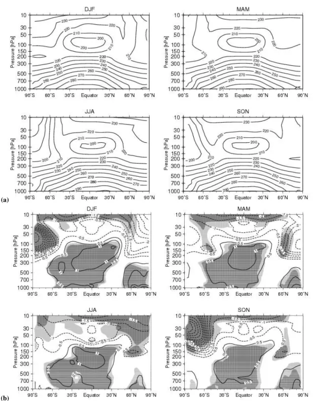
(b)
Fig. 6. (a) Seasonal mean values of zonal mean ozone mixing ratios derived from E39/C transient simulation for the 1960s (1960 to 1969). (b) Differences calculated between mean values derived for the 1960s and corresponding values for the 1990s. Positive (negative) values
indicate more (less) ozone in the 1990s. Light (dark) shading indicates regions in which differences are statistically significant at the 95% (99%) level (t-test). Units are in ppbv.
analyses of observations which also indicate a cooling trend with numbers ranging from 0.3 to 1.4 K per decade (e.g. WMO, 1999). The picture is rather unclear in the tropical
tropopause region. For example, temperature trends derived from observations estimated at 100 hPa (WMO, 1999) range from +0.3 to −0.5 K. Certainly, this is a difficult region to
(a)
(b)
Fig. 7. Same as in Fig. 6, but for temperature. Positive (negative) values indicate higher (lower) temperature in the 1990s. Units are in K.
The interval of contour lines is 0.5 K, minimum values in the southern polar stratosphere are −5.5 K in DJF and −7.0 K in SON.
obtain a clear trend signal, because it is the transition layer with a warming below and a cooling above. As many other models, E39/C simulates a warming in the upper troposphere which maximises at 250 hPa, but this is not in agreement with radiosonde temperature data which indicate a cooling (e.g.
Parker et al., 1997). Long-term temperature changes at mid-dle and higher latitudes of the Northern Hemisphere midmid-dle troposphere (500 hPa) derived from E39/C (Fig. 7b) vary be-tween +0.5 K (JJA) and +1.0 K (DJF), which is less than de-tected at the Meteorological Observatory Hohenpeissenberg
(a)
(b)
Fig. 8. Same as in Fig. 6, but for zonal wind. Positive (negative) values indicate higher (lower) wind speed in the 1990s. Units are in m/s.
The interval of contour lines is 1 m/s plus the 0.5 and −0.5 contour lines, maximum values in the southern stratosphere are 7 m/s in DJF and 10 m/s in SON.
(MOHp), station of the German Weather Service (47.8◦N, 11◦E) where an increase of 0.7±0.3 K per decade has been found since 1967 (Steinbrecht et al., 1998). One reason for this might be that many tropospheric ozone precursors in-cluding their trends are not considered in the E39/C
simula-tion. In general, the long-term temperature changes derived from the E39/C transient model simulation confirm recent estimates from E39/C time-slice experiments (i.e. 1980 and 1990 conditions) presented also in Shine et al. (2003).
(a) (b)
(c) (d)
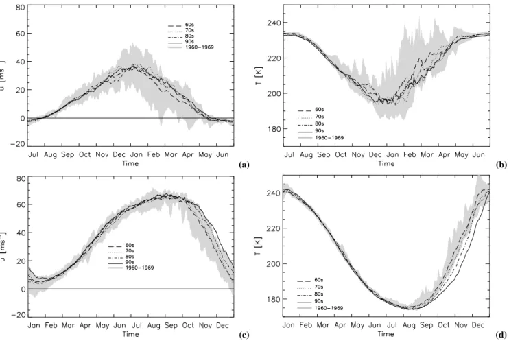
Fig. 9. Climatological mean curves of the annual cycle of the zonal wind (in m/s) at 60◦N (a) and 60◦S (c) at 30 hPa, and of the zonal mean temperature (in K) at 80◦N (b) and 80◦S (d) at 30 hPa. Different lines indicate decadal mean values of the four decades, i.e. the 1960s, 1970s, 1980s, and 1990s. The shaded areas show the range of minimum and maximum values found within the 1960s.
Corresponding changes of the zonal mean wind field are shown in Fig. 8b. The statistically significant increase of the zonal mean wind speed of up to 6 m/s in the South-ern Hemisphere lower stratosphere during spring (SON) and summer months (DJF) reflects the ozone hole formation and the corresponding decrease of polar stratospheric tempera-tures. Another systematic change pattern, which is obvious throughout all seasons, is found at mid-latitudes of the North-ern Hemisphere (the pattNorth-ern is obvious though less distinct in the Southern Hemisphere, as well). Here, the temperature change in the upper troposphere/lower stratosphere intensi-fies the zonal wind due to the thermal wind equation. This results in a more intense tropospheric jet stream in DJF and MAM, and tends to shift the jet stream to lower latitudes in JJA and SON. This is accompanied by a warming of the Arc-tic lower troposphere and a reduction of the horizontal tem-perature gradient at lower altitudes, resulting in a reduction of the zonal mean wind at around 50◦to 60◦N. The strength-ening of the tropospheric jet is consistent with observations, however the weakening of the westerly zonal flow near the surface at northern latitudes from about 50◦to 60◦is not (e.g.
Shindell et al., 2001).
To display dynamical changes of the polar vortices during the 40 model years, an analysis of zonal mean temperature and zonal wind is presented in the style of the NCEP anal-yses (see NCEP web-page: http://code916.gsfc.nasa.gov/ Data-services/met/). Figure 9 shows climatological mean curves of the annual cycle of the zonal wind at 60◦N and S
at 30 hPa (Figs. 9a and c) and of the zonal mean temperature at 80◦N and S at 30 hPa (Figs. 9b and d). The lines represent mean values for the four decades covered by the transient simulation, the shaded area denotes the minimum and maxi-mum values reached during the 1960s of the model. Similar to the results presented in Hein et al. (2001), the model again shows its ability to reproduce hemispheric differences of dy-namical variability changes. While the annual cycle is well captured in both hemispheres, and the mean values in the Northern Hemisphere agree well with respective analyses de-rived from observations, the model shows again deficiencies in the Southern Hemisphere which are related to the cold bias (see discussion above). With regards to the dynamical vari-ability of the Northern Hemisphere during winter and spring, E39/C shows reduced interannual variability in early win-ter. Nevertheless, E39/C is able to reproduce stratospheric
warmings in mid and late winter, but the number of major events is smaller than observed. In the Northern Hemisphere the climatological mean values for the four decades do not indicate systematic changes (mainly due to the high dynam-ical variability), which is supported by analyses of observa-tions (e.g. Labitzke and Naujokat, 2000). In the Southern Hemisphere the lower stratosphere changes steadily towards more stable polar vortices and colder conditions in late win-ter and early spring. The lifetime (persistence) of the polar vortex has been prolonged by about three weeks, as the com-parison of the results of the 1960s with those of the 1990s shows. This is in good agreement with an estimate pre-sented by Zhou et al. (2000) who carried out their analysis on 19 years (1979–1998) of NCEP/NCAR reanalysis data and found that the Southern Hemisphere polar vortex has last about two weeks longer in the 1990s than in the early 1980s. 3.3 Tropopause and water vapour
Lower stratospheric water vapour trends may give a substan-tial contribution to the total radiative forcing of trace gas changes in the recent past (e.g. Rosenlof et al., 2001; Forster and Shine, 2002). However, results from time series anal-ysis of the few available observed data (e.g. Oltmans et al., 2000; Rosenlof et al., 2001; Randel et al., 2004) of strato-spheric water vapour do not produce a uniform picture of the magnitude and even the sign of a respective trend. A possible feedback chain driving stratospheric water vapour trends involves trends in tropopause height (e.g. Steinbrecht et al., 2001; Santer et al., 2003) and related tropopause tem-perature, which at least in the tropics may control changes in the water vapour penetration from the troposphere into the stratosphere (Zhou et al., 2001). While in the present paper we will not investigate in detail the mechanisms responsible for long-term changes of water vapour concentrations in the lower stratosphere (a paper on this individual subject will be prepared later), we will give a brief overview of the overall trend simulated in the transient simulation.
The changes of the thermal tropopause pressure are given in Fig. 10a. Whereas no obvious systematic changes (trends) are seen in the first two decades of the simulation, model results indicate a gradual change in tropopause height after about 1980. In both hemispheres, E39/C simulates a de-crease (inde-crease) of tropopause pressure (height) poleward of around 50◦. The subtropical regions show an increase (de-crease) of tropopause pressure (height). There appears to be no uniform trend throughout the 40-year simulation in the tropics. The major volcanic eruptions included in the tran-sient simulation lead to a temporary increase of tropopause pressure due to tropospheric cooling. Changes in tropopause temperature (not shown) are directly related to the vari-ability of the tropopause height: An increase (decrease) of tropopause height goes along with a decrease (increase) of tropopause temperature. A comparison with an analysis of tropopause height changes at MOHp, 47.8◦N (Steinbrecht et
al., 1998, 2001) shows a qualitative agreement, i.e., a more or less steady increase of tropopause height in February dur-ing the last 30 years. However, the model underestimates the rise in tropopause height compared to the estimates by Stebrecht et al. (2001). Whereas SteinStebrecht et al. finds an in-crease of 125 m/decade for the station MOHp, E39/C calcu-lates only about +80 m/decade for the corresponding model grid point. A possible explanation for the rise of tropopause height might be identified in the warming of the troposphere and accompanying cooling of the stratosphere (Steinbrecht et al., 2001). If this is the case, the difference between model results and observations might be explained by the fact, that the tropospheric warming in the model at Northern Hemi-sphere mid-latitudes is smaller than observed (see discussion above).
Figure 10b depicts the changes of water vapour mixing ra-tio at the thermal tropopause during the 40 year model sim-ulation. A uniform trend is obvious only in the subtropical region, where water vapour mixing ratios are higher in the late 1980s and throughout the 1990s. Long-term changes are not uniform in the tropics, and neither at middle and high lati-tudes of both hemispheres. As discussed before, the volcanic eruptions involve characteristic signatures (see also below).
The general distribution of the pattern change in the lower stratosphere is equal to that at the tropopause. E39/C results, which allow a comparison with measurements of the Boulder frost point hygrometer and corresponding HALOE data dis-cussed in Randel et al. (2004) (their Fig. 8a), are presented in Fig. 11 for the lower stratosphere (80 hPa). The figure shows not only the results at 40◦N, but also at 40◦S, since the temporal development is very similar.
A comparison between the measurement time series of stratospheric water vapour over Boulder (Oltmans et al., 2000) and the respective model data for the period after 1979 indicates a systematic model error with respect to the abso-lute concentration, but good agreement with respect to the observed trend during these two decades (Stenke and Grewe, 2005). While the simulated stratospheric water vapour dis-tribution was significantly improved by including methane oxidation (e.g. Hein et al., 2001), it has also been established that the Boulder trend, as well as other observed trends dur-ing the 1990s are too strong to be explained by methane ox-idation alone (Rosenlof, 2002). Recently, Joshi and Shine (2003) have proposed that part of the observed long-term wa-ter vapour trend may be explained by the observed series of volcanic eruptions, provided that the stratospheric residence time of water vapour is in the order of 5 to 10 years and, thus, considerably longer than the residence time of the vol-canic aerosols. Our model simulations do not reproduce this behaviour, as they indicate a memory of little more than 4 years at about 25 km height (Fig. 11).
Interestingly, E39/C simulates no positive trend in lower stratospheric water vapour mixing ratios in the years before 1980. On the contrary, a negative trend is found in the 1960s. A further discussion about possible reasons for this model
(a)
(b)
Fig. 10. Zonal mean changes of pressure (in hPa, top panel) and of water vapour mixing ratio (in ppmv, bottom panel) at the thermal
tropopause, as simulated with E39/C.
behaviour is given in Sect. 4.3. Compared with the Boul-der measurements one must conclude that the water vapour signals of the large volcanic eruptions are overestimated in E39/C (see discussion in Sect. 4.1). In addition, a more
de-tailed analysis of stratospheric water vapour variability and trends involving further sensitivity studies with the model system is given in Stenke and Grewe (2005).
2136 M. Dameris et al.: Variability in a transient CCM simulation -1 0 1 2 3 [ppmv] 1960 1965 1970 1975 1980 1985 1990 1995 2000 80 hPa
Fig. 11. Temporal development of zonal mean water vapour
anoma-lies (in ppmv) at 40◦N (black curve) and 40◦S (grey curve) at
80 hPa as simulated with E39/C. The given values of differences are with respect to reference values of the years 1960 to 1980.
4 Variability due to external forcings
In this section, the model response to prescribed forcings is investigated. A guiding question for the discussion is how deterministic is the response of the non-linear atmospheric (model) system? We consider both, abrupt perturbations (e.g. volcanic eruptions) and quasi-periodic forcings like the QBO and the 10 to 12 year solar activity cycle. It is im-portant for a better understanding of the climate system to identify key parameters which are most relevant for the de-scription of atmospheric variability and changes and which, therefore, must form the focus of quantitative assessments of future atmospheric changes. As already mentioned, we can-not expect unassailable quantitative conclusions from only one simulation. Since E39/C is driven by observed SSTs, which themselves may include a non-deterministic variabil-ity component from internal ocean fluctuations, there are ob-vious limitations in estimating the deterministic behaviour of the system.
4.1 Volcanic eruptions
Major volcanic eruptions strongly disturb the atmosphere, as many analyses of observed physical, dynamical, and chemical parameters have shown (e.g. Coffey, 1996; Angell, 1997a,b; Andronova et al., 1999; Robock, 2000). Due to up-graded observation techniques, the documentation of effects following the eruption of Mt. Pinatubo in 1991 is the most comprehensive. As described in Sect. 2, the transient simu-lation performed with E39/C considers the effects of volca-noes in the chemistry, as well as in the radiation scheme of the interactive model system.
Figure 12 shows a comparison of global mean tempera-ture anomalies in the lower stratosphere derived from Mi-crowave Sounding Unit (MSU) Channel 4 (1979–2002) and equivalent temperatures (derived according to Santer et al., 1999) from the E39/C transient simulation (1960–1999). The most obvious features are the temperature increases imme-diately following the eruptions of Agung, El Chichon, and Mt. Pinatubo, which reach about 2 K in the simulation. The main part of the model signal originates from tropical lati-tudes, where maxima in the zonal mean response of more than 3 K occur (not shown). It is evident from observations
Fig. 12. Comparison of global mean temperature anomalies in the lower stratosphere (15 to 23 km) derived from observations (MSU Channel 4) and equivalent values calculated from results of the E39/C model simulation.
www.atmos-chem-phys.org/0000/0001/ Atmos. Chem. Phys., 0000, 0001–33, 2005
Fig. 12. Comparison of global mean temperature anomalies in the
lower stratosphere (15 to 23 km) derived from observations (MSU Channel 4) and equivalent values calculated from results of the E39/C model simulation.
that the model overestimates the lower stratosphere tempera-ture response following the eruptions by about 1 K (see also WMO, 1986). Kirchner et al. (1999) found a 2 K excess of their simulated temperature response (near the equator at 70 hPa, see their Fig. 5b) compared to observations, which they explained by the missing QBO modulation of heating rates and missing ozone depletion in their model configu-ration (both effects contributing 1 K). As the QBO has been nudged into our transient experiment (see Sects. 2.2 and 4.2), no inconsistency to observations occurs in this respect. Like-wise, the 1 K cooling effect that observed tropical ozone de-pletion forces on tropical temperatures according to Kirchner et al. (1999), should be included in our simulation in case that the interactive chemistry-climate coupling produces the cor-rect signal. A reduction of tropical ozone similar to the ob-served one is indeed evident in the simulation (Fig. 4, com-pare with Bojkov and Fioletov, 1995). We cannot convinc-ingly explain the apparent inconsistency between the conclu-sions of Kirchner et al. (1999) and our results, but some pos-sibilities are conceivable: The vertical distribution of column ozone depletion may be different in both model systems, ei-ther due to shortcomings of the chemistry-climate model or because the diagnostic method used by Kirchner et al. (1999) was too simple. Similar differences may exist with respect to the QBO induced heating rates. A further possibility is the different water vapour feedback to be expected in both simulations: As the volcano-related heating of the tropical tropopause region is higher than observed in both simula-tions, but more distinct in the Kirchner et al. (1999) config-uration, stratospheric water vapour uptake and its related ra-diative cooling feedback can be expected to be stronger in the simulations of Kirchner et al. (1999). If this is correct, the aerosol absorption heating rates calculated by Kirchner et al. (1999) for the Mt. Pinatubo eruption and adopted in our simulations may overestimate the actual effect after all, as they are able to balance an exaggerated water vapour ra-diative cooling in the original framework, but will overdo with respect to the smaller and more realistic water vapour
(a)
(b)
Fig. 13. Top: Monthly mean deviation of O3production and O3destruction at 50.1◦N, 50 hPa. The deviation has been calculated separately for each month, relative to the associated reference month, as a climatological mean for 1967–1979. Bottom: Monthly mean deviation of
O3concentration for the months April, November, and the difference April-November at 50.1◦N, 50 hPa. The deviation has been calculated
separately for April and November, relative to the associated reference month as a climatologiocal mean for 1967–1979.
feedback in the CCM simulation. A more speculative reason for the overestimation of the volcano signal is the possible injection of moist air masses from the volcano exhaust into the stratosphere that would not be modulated by freeze dry-ing at the tropopause. If such contribution were substantial, a mechanism of moistening and cooling the stratosphere would be absent from both the simulations of Kirchner et al. (1999) and ours.
The heating of the stratosphere caused by volcanic aerosol results not only in an increase of the stratospheric mean tem-perature of about 2 K, it also enhances the meridional cir-culation. The vertical ascent in the tropics is amplified by roughly 20%, which results in an uplift of the ozone
pro-file, i.e., a vertical displacement of the ozone maximum, and a decrease of the total ozone column of approximately 5% (Stenke and Grewe, 2005, see also Fig. 4). The water vapour in the tropical lowermost stratosphere is significantly enhanced, which leads to an increase of OH by 20 to 25% at 70 hPa and a significantly stronger HOxdestruction cycle.
However, chemical timescales in the lower stratosphere are still long compared to the dynamical timescale so that the chemical changes have only an impact on ozone in the order of 0.1% on the total column (Stenke and Grewe, 2005).
In northern mid-latitudes (40◦N–50◦N) at about 50 hPa ozone concentrations are not only dynamically controlled, but also by chemistry. Relative changes of ozone production
Fig. 14. Temporal development of total ozone for the midlatitude
region of 30◦N and 60◦N, calculated for January, February, and
March averages, derived from E39/C model results. Values are given in DU.
and destruction cycles are similar during the three volcanic episodes, except for chlorine. Ozone production is reduced by 30% (top panel of Fig. 13), which is strongly deter-mined by NOxremoval from the gas-phase due to
heteroge-neous conversion (on aerosol) from N2O5to HNO3. Ozone
loss rates involve more complex interactions. The increase of water vapour leads to a more pronounced ozone de-struction due to HOx in the order of 50% to 100%. The
NOx cycle is reduced by 20 to 40% due to a shift within
the NOy components towards more HNO3 from the
reac-tion NO2+OH→HNO3. There are other chemical reactions
which have an additional influence on the NOxcycle (e.g.,
it should be reduced by the reaction N2O5+H2O as well),
but these effects have not been analysed in detail. Ozone de-struction by chlorine is doubled during the El Chichon period and even enhanced by a factor of 10 during the Pinatubo pe-riod compared to the non-volcanic pepe-riod 1967 to 1979. In total, the enhanced ozone depletion by the HOxcycle
dom-inates during the Agung episode. During El Chichon, both the HOx and ClOx cycle are of equal importance. During
the Pinatubo episode the changes in the destruction cycles are clearly dominated by the ClOx cycle. This leads to an
increased ozone destruction of around 20%, 40%, and 80% during the three volcanic episodes of Agung, El Chichon, and Mt. Pinatubo, respectively (Fig. 13a).
Using these changes in the production and loss rates, the effect on ozone is a reduction in the order of 5% per month at 50 hPa in the period March to May, based on a simple calculation applying the ozone production and loss terms from the climate-chemistry simulation. This leads to approx-imately 15% ozone loss at 50 hPa during spring related to the Pinatubo perturbation, which can be revealed by compar-ing early winter (November) and late sprcompar-ing (April) ozone
values at 50 hPa (Fig. 13b). Both the November ozone val-ues and the difference to the April ozone valval-ues are strongly perturbed during the post El Chichon and post Pinatubo pe-riod. Taking into account that 40% of the ozone column is affected by this process, then this reduces the ozone column by roughly 6%, which agrees with observational data (WMO, 2003).
The perturbation of dynamical and chemical values and parameters discussed so far lasted only for a relatively short time period of between 1.5 and 4 years. In addition, Fig. 12 indicates that the modelled temperature trend is in good agreement with the MSU analysis. Interestingly, similar to the changes derived from MSU data, the model results also indicate stepwise changes towards lower temperatures in the lower stratosphere after the eruptions of El Chichon and Mt. Pinatubo, which is not simulated after the eruption of Agung. No temperature trend is detected in the years after El Chichon and Pinatubo, neither in MSU analysis nor in E39/C data (see also Pawson and Naujokat, 1997). Dedicated addi-tional simulations would be necessary for a conclusive inter-pretation, but a plausible explanation could be the following: The eruption of Agung happened during low solar activity whereas El Chichon and Mt. Pinatubo erupted shortly after and during solar maximum, respectively. The solar cycle ef-fect probably masks the anticipated, more or less linear nega-tive temperature trend, which is caused by enhanced concen-trations of GHGs. Slightly enhanced (reduced) temperatures are expected in the lower stratosphere during higher (lower) solar activity due to higher (lower) short-wave heating rates (e.g. Matthes et al., 2004). The calculated temperature differ-ences (i.e. annual, global mean) between solar maximum and minimum in the lower stratosphere (around 15 to 25 km) are approximately 0.2 K (Matthes et al., 2003), which is the same order of magnitude that is expected from the anthropogenic greenhouse effect. Therefore, in the years from 1985 to 1991 and after 1996 with increasing solar activity, the cooling of the lower stratosphere due to increasing concentrations of GHGs might be compensated such that no net temperature trend is obvious.
4.2 The quasi-biennial oscillation
Looking more carefully at the modelled temperature anoma-lies (Fig. 12), in particular in the years between 1965 and 1982, the QBO signal can be detected, which also contributes to the overall variability. A modulation of dynamical and chemical quantities caused by the prescribed QBO is also obvious in Fig. 4 in the equatorial region. Qualitatively, the QBO signal is in good agreement with a similar analysis de-rived from merged satellite and ground based data (Bojkov and Fioletov, 1995; updated version until the year 2000 is at our disposal, Fioletov, pers. communication). The anoma-lies derived from observations and the model results are of the same order of magnitude until the 1980s (i.e., up to 6%). They are notably smaller during the 1990s in E39/C, where
observed fluctuations have continued with similar magni-tudes. Here the modelled ozone varies only by about 2– 3%. It seems that in E39/C the QBO signal in total ozone is partly masked by the (too) strong ozone anomalies after the volcanic eruptions. QBO signatures in E39/C can be de-tected in total ozone in all latitudinal regions. For exam-ple, at mid-latitudes of the Northern Hemisphere (Fig. 14), E39/C shows amplitudes in total ozone of 12 DU±4 DU dur-ing winter months (JFM) which can be clearly related to the QBO. Similar results have been found in an analysis based on TOMS data (Burrows et al., 2000; see also Fig. 2.4 in EC-report, 2001). A linear regression analysis of long-term mea-surements of ozone at MOHp, 47.8◦N indicates QBO-related fluctuations of ±10 DU (peak-to-trough ozone changes up to 20 DU) in February (Steinbrecht et al., 2001). The dominant effect of the QBO in the lower stratosphere is the variation of the meridional circulation and the tropical ascent. For ex-ample, in the case of a westerly phase of the QBO the merid-ional circulation converges horizontally towards the jet core so that the upwelling is strongly reduced (increased) in the shear layer below (above) the jet. The opposite modification is found for the meridional circulation in the vicinity of the easterly jet. The QBO signal in tropical upwelling explains enhanced water vapour and reduced NOyand ozone mixing
ratios, all in the range of 5% to 10% around 50 hPa. This is consistent with the behaviour of tropospheric tracers, which are included in the model (Grewe, 2004). They do all show increased values at 50 hPa during episodes of QBO-induced enhanced upwelling. This explains to a large extent the vari-ations of the chemical species. Since water vapour has an op-posite vertical gradient compared to NOyand ozone, the
vari-ations are anti-correlated. Varivari-ations of lower stratospheric ozone depletion in the tropics caused by the QBO are in the order of ±15 to 20%. If chemistry leads, than increased loss rates should cause lower ozone values. This is not the case: Ozone is increased (due to transport) and then ozone loss rates are increased. Positive (negative) ozone anomalies re-sult in enhanced (reduced) NOxand HOxdestruction cycles.
This gives a clear indication that the variations of the de-struction cycles are a consequence of the ozone variations and not vice versa; since otherwise ozone anomalies should be correlated with the ozone loss rates. Therefore, the QBO signal in column ozone is dynamically induced with some negative feedbacks from chemistry. Returning to Fig. 12, quasi-biennial fluctuations in the global mean temperature anomalies of the lower stratosphere are visible in the E39/C data, in particular in the years between 1966 and 1982, which is a long period without major volcanic activity. After the eruptions of El Chichon and Mt. Pinatubo a similar signature cannot be identified, neither in E39/C nor in the MSU data analysis.
Fig. 15. Total ozone deviations (in %) for the latitude range 25◦S to 25◦N. Anomalies are calculated from E39/C results with respect to the model data during the years 1964 to 1980.
4.3 The solar cycle
The impact of solar activity, in particular of the 11-year solar cycle, on climate and the stratosphere has often been investi-gated (e.g. Haigh, 1996). For example, total ozone anomalies in the tropics (25◦N to 25◦S) have been discussed in WMO (2003; Fig. 4–5 therein), based on combined observations for the years from 1978 to 2003 (synergistic use of ground-based and satellite data). Decadal variations of total ozone in the tropics (peak-to-trough variations of about 3%) suggest a correspondence with the activity cycle of the sun: The max-ima are approxmax-imately in phase with the 11-year solar cycle. Our transient simulation includes the effects of changing photolysis rates below 30 km altitude and also chemically induced ozone changes caused by prescribed time evolution of NOy at the model top. Calculated ozone anomalies in
the tropical belt derived from E39/C (Fig. 15) develop simi-larly to observations (WMO, 2003), with positive anomalies around solar maxima (1981 and 1991) and negative anoma-lies around solar minima (1986 and 1996). While this is no proof for a dominating impact of solar cycle fluctuations on the tropical ozone layer, the phenomenological similarity be-tween observed and modelled development indicates that a detailed investigation may be worthwhile. A respective pa-per dealing with the separation of the solar signal in dynamic and chemical components is in preparation. Interestingly, be-fore 1978 the solar signal is less but still suggested by higher ozone values around 1960 and 1969 in comparison to 1965. Note that the solar cycle between 1965 and 1976 was less dis-tinct, according to 10.7 cm radiation intensity records, than the other cycles included in the period. Recalling discussions in previous sections a distinct QBO signal is immediately ev-ident in Fig. 15.
To get a better insight into the radiative impact of solar activity changes on dynamics and chemistry in E39/C, it is helpful to have a look at the long-term variability of ozone
Fig. 16. Temporal development of ozone production rates (left, in cm−3s−1) and ozone photolysis rates (right, in s−1) at 10 hPa (top), 30 hPa (middle), and 50 hPa (bottom), for the latitude range 25◦S to 25◦N.
photolysis and production rates during the 40 year transient simulation. Figure 16 shows respective results of E39/C at 10, 30, and 50 hPa at lower latitudes (25◦N to 25◦S). The values calculated at 10 hPa directly reflect the prescribed changes of the extra-terrestrial flux at the upper boundary of E39/C. This must be kept in mind because the low upper boundary conditionally implies some uncertainties on causes and effects in this case. For example, the largest percent-age ozone changes have been found in the upper stratosphere (e.g. Haigh, 1996). While this does not significantly change the total ozone column, it might have a dynamical influence on the lower and middle stratosphere. In the model, the so-lar signal can, to some part, still be identified at 30 hPa, the picture changes further down in the lower stratosphere. At 50 hPa, the 11-year solar cycle is no longer obvious because of feedback processes (e.g., interactive ozone) and the influ-ence of volcanic eruptions. Here, changes of ozone photoly-sis and production on longer time scales are identified, with minimum ozone photolysis and production rates in 1975 and
higher values before and after that year. Interestingly, corre-sponding similar long-term changes are found in other model data sets: For example, in Sect. 3.3 it is shown that water vapour mixing ratios at mid-latitudes of the lower strato-sphere slightly increase in the 1980s and 1990s, which is supported by observations at the Boulder station (Oltmans et al., 2000). Model results for the 1970s indicate lowest water vapour mixing ratios without a visible trend and de-creasing mixing ratios in the 1960s, whereas the values in the early 1960s are similar to those of the late 1990s. We explain these changes of water vapour mixing ratios with a corresponding behaviour of the cold-point temperature (not shown), which modifies the transport of water vapour from the troposphere into the stratosphere: A decrease of the cold-point temperature is found from 1960 until the early 1970s (i.e. around 1 K) and an increase of approximately 0.5 K is calculated from the beginning 1980s to 1999. Based on the currently available model results we speculate, although we cannot definitely conclude on the basis of this analysis,