HAL Id: hal-01795319
https://hal.archives-ouvertes.fr/hal-01795319
Submitted on 18 Sep 2018
HAL is a multi-disciplinary open access
archive for the deposit and dissemination of
sci-entific research documents, whether they are
pub-lished or not. The documents may come from
teaching and research institutions in France or
abroad, or from public or private research centers.
L’archive ouverte pluridisciplinaire HAL, est
destinée au dépôt et à la diffusion de documents
scientifiques de niveau recherche, publiés ou non,
émanant des établissements d’enseignement et de
recherche français ou étrangers, des laboratoires
publics ou privés.
Unified Stochastic Reverberation Modeling
Roland Badeau
To cite this version:
Roland Badeau. Unified Stochastic Reverberation Modeling. 26th European Signal Processing
Con-ference (EUSIPCO), Sep 2018, Rome, Italy. �hal-01795319�
Unified Stochastic Reverberation Modeling
Roland Badeau
LTCI, Télécom ParisTech, Université Paris-Saclay, Paris, France Email: [email protected]
Abstract—In the field of room acoustics, it is well known that reverberation can be characterized statistically in a particular region of the time-frequency domain (after the transition time and above Schroeder’s frequency). Since the 1950s, various formulas have been established, focusing on particular aspects of reverberation: exponential decay over time, correlations between frequencies, correlations between sensors at each frequency, and time-frequency distribution. In this paper, we introduce a new stochastic reverberation model, that permits us to retrieve all these well-known results within a common mathematical framework. To the best of our knowledge, this is the first time that such a unification work is presented. The benefits are multiple: several new formulas generalizing the classical results are established, that jointly characterize the spatial, temporal and spectral properties of late reverberation.
Index Terms—Reverberation, room impulse response, room frequency response, stochastic models, Poisson processes, station-ary processes, Wigner distribution.
I. INTRODUCTION
When a microphone records a sound produced by an audio source in a room, the received signal is made of several contributions [1]: firstly, the direct sound, that corresponds to the direct propagation of the sound wave from the source to the microphone, then a few early reflections, that are due to the sound wave reflections on the various room surfaces (walls, floor, ceiling. . . ), and finally the late reverberation: after a time called transition time [2], [3], reflections are so frequent that they form a continuum and, because the sound is partially absorbed by the room surfaces at every reflection, the sound level decays exponentially over time. This phenomenon is called reverberation, and it can be modeled as the convolution between the source signal and a causal room impulse response (RIR), made of a few isolated impulses before the transition time, and of a continuous, exponentially decaying, random process in late reverberation. The Fourier transform of the RIR is called room frequency response (RFR), and the modal theory [4]–[6] shows that its profile is qualitatively similar to that of the RIR: below a frequency called Schroeder’s frequency, the RFR is made of a few isolated modes, and above this frequency the modes become so dense that they can be represented as a continuous random process [7]–[9].
To sum up, reverberation can be modeled as a stochastic process in a rectangular region of the time-frequency do-main [10], as depicted in Fig. 1. If in addition the dimensions of the room are much larger than the wavelength, and the source and the microphones are located at least a half-wavelength away from the walls, then in this time-frequency
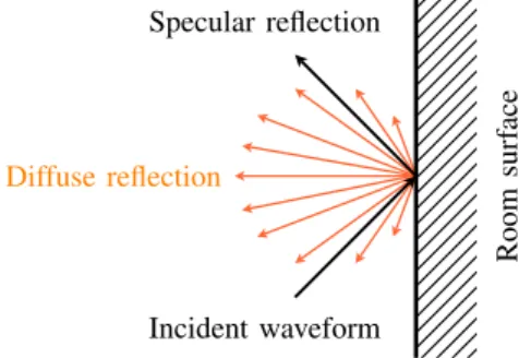
region, the sound field can generally be approximated as diffuse [11]–[13]. Diffusion is a consequence of the reflections on the room surfaces not being specular (i.e. mirror-like), but rather scattered in various directions, as represented in Fig. 2. After many reflections, the sound field can be considered as isotropic: the sound waves come uniformly from all directions.
t f
Validity domain of the stochastic model
t Direct sound Early reflections Late reverberation Transition time f Iso la te d ro o m m o d es Dens e room modes Schr oeder ’s fr equenc y
Room impulse response (RIR)
Room fr equenc y res pons e (RFR)
Fig. 1. Time-frequency profile of reverberation (adapted from [10] and [14]).
Historically, the first stochastic reverberation model is due to Schroeder [7] and Moorer [15]: the RIR at microphone i is hi(t) = bi(t)e ↵t1t 0 (1)
where ↵ > 0 and bi(t)is a centered white Gaussian process.
Parameter ↵ is related to the reverberation time Trin seconds
by the equation Tr = 3 ln(10)↵ . The Gaussian distribution of
bi(t) arises from the central limit theorem: in late
reverbera-tion, hi(t)is the sum of many independent contributions.
Schroeder [7]–[9] also noticed that the independency of the samples hi(t)implies that the RFR, defined as their Fourier
transform Fhi(f ), is a stationary random process. From (1), he
derived several formulas that can be summarized by expressing the complex autocorrelation function of Fhi(f ):
corr [Fhi(f1),Fhi(f2)] =
1 1 + ı⇡f1 f2
↵
. (2) Following a similar approach in the spectral domain, under the diffuse field assumption, Cook [16] computed the correlation at frequency f between two sensors at distance D:
corr [Fh1(f ),Fh2(f )] = sinc ⇣ 2⇡f D c ⌘ . (3) Equation (3) was later generalized to combinations of pressure and velocity sensors [17] and to differential microphones [18]. Finally, Polack [19] generalized model (1) by assuming that bi(t)is a centered stationary Gaussian process, whose power
spectral density (PSD) B(f) has slow variations1. Then he
showed that the Wigner distribution [20] of the RIR is Whi,hi(t, f ) = B(f )e
2↵t1
t 0. (4)
In order to account for the fact that the attenuation coeffi-cient ↵ actually depends on the frequency f, he also proposed an empirical generalization of (4):
Whi,hi(t, f ) = B(f )e 2↵(f )t1t 0. (5)
In other respects, based on the billiard theory, Polack [2], [3] also showed that the durations of the various trajectories in a room, from a given source position to the microphone, are distributed according to a Poisson process [21].
Room sur face Incident waveform Specular reflection Diffuse reflection
Fig. 2. Specular vs. diffuse reflection.
In this paper, we propose a unified stochastic model of reverberation, that will permit us to retrieve all formulas (1) to (4) in a common mathematical framework2, to establish a link
with the Poisson distribution proposed by Polack, and to show how the probability distribution of the RIR, which is impulsive in early reverberation, converges to the Gaussian distribution in late reverberation. In addition, this model will also permit us to go deeper into the description of the statistical properties of the RIR over the space, time and frequency domains, and to prove several new results. Finally, we will explain why this model can actually be applied in the whole time-frequency domain in signal processing applications.
This paper is structured as follows: Section II presents important mathematical definitions and notation that will be used throughout the paper. Then our general stochastic re-verberation model is introduced in Section III. The statistical properties of this model at one sensor are investigated in Section IV. The statistical relationships between two sensors are then analyzed in Section V. Finally, some conclusions and
1Note that in this case, F
hi(f )is no longer a stationary process. 2A straightforward generalization of this model also permits to prove (5),
that will be presented in a future paper; a few hints will be given in Section VI.
perspectives are presented in Section VI. Note that this is a fully theoretical work: our purpose was to unify several results that have already been validated experimentally. In order to make the main discussion as clear as possible, all mathematical proofs were moved to Appendices A to C in [22].
II. MATHEMATICAL DEFINITIONS
• R, C: sets of real and complex numbers, respectively • R+: set of nonnegative real numbers
• ı =p 1: imaginary unit
• [a, b]: closed interval, including a and b 2 R • ]a, b[: open interval, excluding a and b 2 R
• L2([a, b]): square-integrable functions of support [a, b] • x(bold font), z (regular): vector and scalar, respectively • k.k2: Euclidean/Hermitian norm of a vector or a function • z: complex conjugate of z 2 C
• x>: transpose of vector x
• S2: unit sphere in R3(S2={x 2 R3;kxk2= 1}) • E[X]: expected value of a random variable X • X(✓) =E[eı✓X]: characteristic function of X
• Covariance of two complex random variables X and Y :
cov[X, Y ] =E[(X E[X])(Y E[Y ])] (6)
• var[X] = cov[X, X]: variance of a random variable X • Correlation of two complex random variables X and Y :
corr[X, Y ] = pcov[X, Y ]
var[X] var[Y ] (7)
• P( ): Poisson distribution of parameter > 0:
N⇠ P( ) , P (N=n) = e n!n , N(✓) = e (e
ı✓ 1)
(8)
• sinc(x) =sin(x)x : cardinal sine function
• 1A: indicator function (1A(x)is 1 if x 2 A or 0 if x /2 A) • (t) = ( t): conjugate and time-reverse of : R ! Ce • Convolution of two functions 1and 2:R ! C:
( 1⇤ 2)(t) =
R
u2R 1(u) 2(t u)du • Fourier transform of a function : R ! C:
F (f ) =Rt2R (t)e 2ı⇡f tdt (f 2 R) (9) • Two-sided Laplace transform of a function : R ! C:
L (s) =Rt2R (t)e stdt (s2 C) (10) • Wigner distribution (a.k.a. Wigner-Ville distribution) of
two second-order random processes 1(t)and 2(t):
W 1, 2(t, f )=
R
Rcov[ 1(t+u2), 2(t-u2)]e-2ı⇡f udu. (11)
III. DEFINITION OF THE STOCHASTIC MODEL
The model that we present in this section is based on the source image principle [1], [23]. As illustrated in Fig. 3 in the case of specular reflections in a rectangular room3,
the trajectory inside the room from the real source to the
3Fig. 3 illustrates the source image principle in 2D-space for convenience,
microphone is equivalent to a virtual straight trajectory from a so-called source image which is outside the room. A remark-able property of this principle is that, regardless of the room dimensions, the density of the source images is uniform in the whole space: the number of source images contained in a given disk, of radius sufficiently larger than the room dimensions, is approximately invariant under any translation of this disk.
Fig. 3. Positions of microphone (green plus), source (thick blue point) and source images (black points). The original room walls are drawn with thick lines. A virtual straight trajectory from one source image to the microphone is drawn with colors, along with the real trajectory in the original room.
Since we aim to define a general stochastic reverberation model, independent of the geometry of the room, we will consider that the positions of the source images are random and uniformly distributed (note that this assumption is a fortiori valid in the case of a diffuse sound field, which is uniform). More precisely, we will assume that the number N (V )of source images contained in any Borel set V ⇢ R3
follows a Poisson distribution of parameter |V |, where |V | is the Lebesgue measure (volume) of V . Mathematically, this is formalized by considering a Poisson random measure with independent increments dN(x) ⇠ P( dx).
In other respects, we will assume that the sound waves undergo an exponential attenuation along their trajectories, that is due to the multiple reflections on the room surfaces and to the propagation in the air. In this paper we focus on the case of omnidirectional microphones, so we will further assume that this attenuation is isotropic (in accordance with the diffuse field approximation) and independent of the frequency. It will thus only depend on the length of the trajectory, as in [19].
Finally, we suppose that several microphones4 indexed by
an integer i are placed at arbitrary positions xi in the room.
We end up with the following model: hi(t) =
R
x2R3hi(t, x) e
↵
ckx xik2dN (x), (12)
where hi(t)is the RIR at microphone i, ↵ > 0 is the
attenu-ation coefficient (in Hz), and c > 0 is the sound speed in the air (approximately 340 m/s in usual conditions). The impulse hi(t, x), propagated from the source image at position x, is
modeled as a coherent sum of monochromatic spherical waves:
4For the sake of simplicity, we will focus on the case of two microphones;
the generalization to an arbitrary number of microphones is straightforward.
hi(t, x) = Z f2R A(f )e 2ı⇡f⇣t kx xik2c ⌘ kx xik2 df, (13) where A(f) is a linear-phase frequency response (in order to ensure coherence). In Appendix A in [22], we show that (12) and (13) are equivalent to the following model:
Definition 1 (Unified stochastic reverberation model). Let ↵ > 0, c > 0, and T > 0. Let dN(x) be a uniform Poisson random measure on R3 with independent increments:
dN (x)⇠ P( dx). (14) Let g(t) 2 L2([ T, T ]), such that
Fg(0) =dFg
df (0) = 0, (15) 8f 2 R, Lg(↵ + 2ı⇡f ) 0. (16)
At any sensor position xi2 R3, hi(t)is defined as
8t 2 R, hi(t) = e ↵(t T )bi(t), (17) where bi(t) = Z x2R3 g ✓ t T kx xik2 c ◆ dN (x) kx xik2. (18)
Equivalently, the Fourier transform of hi(t)is
Fhi(f ) =Lg(↵+2ı⇡f )e 2ı⇡f TZ R3 e ↵+2ı⇡fc kx xik2 kx xik2 dN (x). (19) This definition calls for comments. Firstly, the linear-phase frequency response A(f) in (13) was parameterized as
A(f ) =Lg(↵ + 2ı⇡f )e 2ı⇡f T. (20)
This technical definition aims to simplify the mathematical developments in the next sections. Secondly, any function g 2 L2([ T, T ])is such that F
g(f )and f 7! Lg(↵ + 2ı⇡f )are
infinitely differentiable, so Fg(0), ddfFg(0)and Lg(↵ + 2ı⇡f )
are well-defined. The constraints (15) and (16) imposed to g are required to prove Propositions 2 and 3 in Sections IV and V. In particular, the support of g is chosen so that hi(t)
in (17) and bi(t) in (18) are causal. Thirdly, the existence
of functions g that satisfy these constraints is guaranteed by Lemma 1 in Appendix A in [22].
Now it is time to investigate the properties of this model. In Section IV, we will focus on one sensor at spatial position xi.
Then in Section V, we will analyze the spatial relationships between two sensors at different positions xiand xj.
IV. STATISTICAL PROPERTIES AT ONE SENSOR
Let us first introduce an equivalent model definition: Proposition 1 (Equivalent model definition at one sensor). With the same notation as in Definition 1, we have:
bi(t) = Z r2R+ g⇣t T r c ⌘ dN(r) r , (21) Fhi(f ) =Lg(↵ + 2ı⇡f )e 2ı⇡f T Z r2R+ e ↵+2ı⇡fc rdN (r) r (22)
where dN(r) are independent Poisson increments on R+:
dN (r)⇠ P(4⇡ r2dr). (23)
Proposition 1 is proved in Appendix A in [22]. Let us now investigate the statistical properties of this model:
Proposition 2 (Statistical properties at one sensor position). The model in Definition 1 has the following properties:
1) First order moments:
• in the spectral domain: 8f 2 R,
E[Fhi(f )] =
4⇡ c2L
g(↵ + 2ı⇡f ) e 2ı⇡f T
(↵ + 2ı⇡f )2 , (24)
• in the time domain:
8t 2T, E[hi(t)] =E[bi(t)] = 0. (25)
2) Second order moments:
• in the spectral domain: 8f, f1, f22 R,
var[Fhi(f )] = 2⇡ cLg(↵ + 2ı⇡f ) 2/↵, (26) corr[Fhi(f1),Fhi(f2]) = e 2ı⇡(f1 f2)T 1 + ı⇡f1 f2 ↵ . (27)
• in time domain: 8t 2T , bi(t)is a wide sense
sta-tionary (WSS) process, of autocovariance function 8⌧ 2 R, (⌧) = cov[bi(t+⌧ ), bi(t)] = 4⇡ ceg⇤g(⌧) (28) autocorrelation function 8⌧ 2 R, (⌧) = corr[bi(t + ⌧ ), bi(t)] = (eg ⇤ g)(⌧) kgk2 2 (29) and power spectral density
8f 2 R, B(f) = F (f) = 4⇡ c |Fg(f )|2. (30)
Consequently,
8t 2T, var[hi(t)] = 4⇡ ckgk22e 2↵(t T ) (31)
8t1, t2 2T, corr[hi(t1), hi(t2)]= (t1 t2)(32) • in the time-frequency domain:
8f 2 R, 8t 2T, Whi,hi(t, f ) = B(f ) e
2↵(t T ).
(33) 3) Asymptotic normality: when t ! +1 (i.e. t T), bi(t)
is distributed as a stationary Gaussian process. Proposition 2 is proved in Appendix B in [22]. Note that (30) and (15) show that B(f) is very flat at f = 0: B(0) =dBdf(0) =ddf2B2(0) =d
3B
df3(0) = 0. The asymptotic
nor-mality is related to the central limit theorem: when r becomes large, the volume contained between the spheres of radius r and r+dr increases as r2dr, and so does the number of source
images included in this volume as shown in (23), which leads to the addition of an increasing number of independent and identically distributed (i.i.d.) random increments dB(x).
This proposition permits us to retrieve most of the classical results listed in the introduction. Firstly, hi(t)is centered for
t 2T (the fact that it is not centered for t 2 [0, 2T ] explains why the expected value of the frequency response E[Fhi(f )]in (24) is not zero). Secondly, (17) corresponds to
Schroeder and Moorer’s model defined in (1) when T ! 0 (in this case the process bi(t)becomes white, and it is Gaussian
when t T), and in the general case it is equivalent to Polack’s model [19, chap. 1] (bi(t) is a centered stationary
Gaussian process when t T). When T ! 0, (27) reduces to Schroeder’s formula (2), which was indeed established by assuming that bi(t) is white. Finally, (33) is equivalent to
Polack’s time-frequency model defined in (4). To the best of our knowledge, the other formulas in Proposition 2 are novel.
V. STATISTICAL PROPERTIES BETWEEN TWO SENSORS
Let us now focus on the relationships between two sensors: Proposition 3 (Statistical properties between two sensors). Let us consider the model in Definition 1 at two positions xi
and xj2 R3. Let us define the rectangular window
8t 2 R, w(t) =2Dc 1[ D
c,Dc](t), (34)
where D = kxi xjk2. Then, in addition to the properties
listed in Proposition 2, we also have:
• in the spectral domain: 8f1, f22 R,
corr[Fhi(f1),Fhj(f2)] = e ↵D c 2ı⇡(f1 f2)(T +D2c)sinc(⇡(f1+fc 2)D) 1+ı⇡f1 f2↵ (35)
• in the time domain: 8t 2T +Dc, b(t) = [bi(t), bj(t)]>is
a centered WSS process, of cross-autocovariance function 8⌧ 2 R, i,j(⌧ ) = cov[bi(t + ⌧ ), bj(t)] = w⇤ (⌧) (36)
cross-autocorrelation function
8⌧ 2 R, i,j(⌧ ) = corr[bi(t + ⌧ ), bj(t)] = w⇤ (⌧) (37)
and cross-power spectral density
8f 2 R, Bi,j(f ) =F i,j(f ) = B(f )sinc(
2⇡f D c ). (38) Consequently,
8t1, t2 2T +Dc, corr[hi(t1), hj(t2)] = w⇤ (t1 t2) .
(39)
• in the time-frequency domain: 8f 2 R,
8t 2T +D
2c,Whi,hj(t, f ) = B(f )e
2↵(t T )sinc(2⇡f D c ).
(40)
• asymptotic normality: when t ! +1 (i.e. t T), b(t) is distributed as a stationary Gaussian process.
Proposition 3 is proved in Appendix C in [22]. Applying equation (35) to f1 = f2 = f, we get Cook’s formula (3)
when ↵ ! 0 (no exponential decay). This formula was indeed originally proved by considering plane waves under a far-field assumption [16]. Besides, equation (39) shows that hi(t)and
hj(t)are correlated on a time interval that corresponds to the
wave propagation from one sensor to the other. To the best of our knowledge, all formulas in Proposition 3 are novel.
VI. CONCLUSION AND PERSPECTIVES
In this paper, we proposed a new stochastic model of reverberation, that permitted us to retrieve various well-known results within a common framework. This unification work resulted in several new results, that jointly characterize the properties of late reverberation in the space, time, and fre-quency domains. The most noticeable result in our opinion is (40), which very simply makes the connection between Polack’s time-frequency model (4) and Cook’s formula (3).
Although this model was motivated by physical assumptions that only hold in a particular region of the time-frequency domain (after the transition time and above Schroeder’s fre-quency), from a signal processing perspective however, one of its most interesting features is that it is also applicable before the transition time and below Schroeder’s frequency. Indeed, since the parameter of the Poisson distribution dN(r) in (23) increases quadratically with the distance r, the model permits to describe both the impulsiveness of the RIR before the transition time, and its asymptotic normality in late re-verberation. Moreover, the frequency response Lg(↵ + 2ı⇡f )
in (19) is able to fit both the smooth PSD B(f) at high frequencies, and sharp resonances due to isolated modes below Schroeder’s frequency. Therefore we end up with a stochastic model involving very few parameters (↵, , filter g, and the distances between microphones), that is able to accurately describe reverberation in the whole time-frequency domain. We thus believe that this model has an interesting potential in a variety of signal processing applications.
However this reverberation model, as it is presented in this paper, is not yet suitable for modeling real RIRs. Indeed, one assumption has to be relaxed: the attenuation coefficient ↵ is not constant but rather depends on frequency in prac-tice, as in Polack’s generalized time-frequency model (5). In a future paper, we will thus present a generalization of the proposed model where we will introduce a frequency-varying attenuation coefficient. Fortunately, a simplification holds asymptotically (in late reverberation), that makes all mathematical derivations still analytically tractable. In partic-ular, we will be able to present a formula that generalizes both (5) and (40). A second generalization of this model would be to represent acoustic fields that are not perfectly diffuse. Apparently, obtaining a mathematical characterization of such acoustic fields should be feasible, because a similar simplification holds asymptotically. Finally, the generalization to directional microphones is straightforward, by using the same approach as presented in [18].
Our future contributions will also focus on the signal pro-cessing aspects of this work: we will show how the generalized model (with a frequency-varying attenuation coefficient) can be formalized in discrete time, and we will propose a fast algorithm that permits to estimate the model parameters with a complexity of O(L log(L)2), where L is the length of the
RIR in samples. Finally, our ultimate goal is to investigate the potential of this model in applications such as source separation, dereverberation, and synthetic reverberation.
REFERENCES
[1] H. Kuttruff, Room Acoustics, Fifth Edition. CRC Press, 2014. [2] J.-D. Polack, “Modifying chambers to play billiards: the foundations of
reverberation theory,” Acta Acustica united with Acustica, vol. 76, no. 6, pp. 256–272(17), Jul. 1992.
[3] ——, “Playing billiards in the concert hall: The mathematical founda-tions of geometrical room acoustics,” Applied Acoustics, vol. 38, no. 2, pp. 235 – 244, 1993.
[4] D.-Y. Maa, “Distribution of eigentones in a rectangular chamber at low frequency range,” The Journal of the Acoustical Society of America, vol. 10, no. 3, pp. 235–238, 1939.
[5] R. Balian and C. Bloch, “Distribution of eigenfrequencies for the wave equation in a finite domain: I. three-dimensional problem with smooth boundary surface,” Annals of Physics, vol. 60, no. 2, pp. 401–447, 1970. [6] J.-D. Polack, “The relationship between eigenfrequency and image source distributions in rectangular rooms,” Acta Acustica united with Acustica, vol. 93, pp. 1000–1011, 2007.
[7] M. R. Schroeder, “Frequency-correlation functions of frequency re-sponses in rooms,” The Journal of the Acoustical Society of America, vol. 34, no. 12, pp. 1819–1823, 1962.
[8] M. R. Schroeder and K. H. Kuttruff, “On frequency response curves in rooms. Comparison of experimental, theoretical, and Monte Carlo results for the average frequency spacing between maxima,” The Journal of the Acoustical Society of America, vol. 34, no. 1, pp. 76–80, 1962. [9] M. R. Schroeder, “Statistical parameters of the frequency response
curves of large rooms,” The Journal of the Acoustical Society of America, vol. 35, no. 5, pp. 299–306, 1987.
[10] J.-M. Jot, L. Cerveau, and O. Warusfel, “Analysis and synthesis of room reverberation based on a statistical time-frequency model,” in Audio Engineering Society Convention 103, Sep. 1997.
[11] T. Schultz, “Diffusion in reverberation rooms,” Journal of Sound and Vibration, vol. 16, no. 1, pp. 17 – 28, 1971.
[12] W. B. Joyce, “Sabine’s reverberation time and ergodic auditoriums,” The Journal of the Acoustical Society of America, vol. 58, no. 3, pp. 643– 655, 1975.
[13] L. Cremer, H. A. Müller, and T. J. Schultz, Principles and applications of room acoustics. London: Applied Science Publishers, 1982, vol. 1. [14] A. Baskind, “Modèles et méthodes de description spatiale de scènes sonores : application aux enregistrements binauraux,” Ph.D. dissertation, Université Pierre et Marie Curie (UPMC), Paris, France, 2003. [15] J. A. Moorer, “About this reverberation business,” Computer Music
Journal, vol. 3, no. 2, pp. 13–28, 1979.
[16] R. K. Cook, R. V. Waterhouse, R. D. Berendt, S. Edelman, and M. C. Thompson Jr., “Measurement of correlation coefficients in reverberant sound fields,” The Journal of the Acoustical Society of America, vol. 27, no. 6, pp. 1072–1077, 1955.
[17] F. Jacobsen and T. Roisin, “The coherence of reverberant sound fields,” The Journal of the Acoustical Society of America, vol. 108, no. 1, pp. 204–210, 2000.
[18] G. W. Elko, “Spatial coherence functions for differential microphones in isotropic noise fields,” Mcrophone arrays, pp. 61–85, 2001. [19] J. D. Polack, “La transmission de l’énergie sonore dans les salles,” Ph.D.
dissertation, Université du Maine, 1988.
[20] L. Cohen, “Time-frequency distributions-a review,” Proc. IEEE, vol. 77, no. 7, pp. 941–981, Jul. 1989.
[21] S. N. Chiu, D. Stoyan, W. S. Kendall, and J. Mecke, Stochastic Geometry and Its Applications, 3rd ed. Wiley, 2013.
[22] R. Badeau, “Research report on unified stochastic reverberation modeling,” Télécom ParisTech, Paris, France, Tech. Rep., Feb. 2018. [Online]. Available: http://service.tsi.telecom-paristech.fr/cgi-bin/ valipub_download.cgi?dId=333
[23] J. B. Allen and D. A. Berkley, “Image method for efficiently simulating small-room acoustics,” Journal of the Acoustical Society of America, vol. 65, no. 4, pp. 943–950, 1 1979.
![Fig. 1. Time-frequency profile of reverberation (adapted from [10] and [14]).](https://thumb-eu.123doks.com/thumbv2/123doknet/14391140.508162/2.892.461.803.431.705/fig-time-frequency-profile-reverberation-adapted.webp)