HAL Id: hal-02935359
https://hal.sorbonne-universite.fr/hal-02935359
Submitted on 10 Sep 2020
HAL is a multi-disciplinary open access
archive for the deposit and dissemination of
sci-entific research documents, whether they are
pub-lished or not. The documents may come from
teaching and research institutions in France or
abroad, or from public or private research centers.
L’archive ouverte pluridisciplinaire HAL, est
destinée au dépôt et à la diffusion de documents
scientifiques de niveau recherche, publiés ou non,
émanant des établissements d’enseignement et de
recherche français ou étrangers, des laboratoires
publics ou privés.
by joint decomposition of brain and behavior
Jennifer Stiso, Marie-Constance Corsi, Jean Vettel, Javier Garcia, Fabio
Pasqualetti, Fabrizio de Vico Fallani, Timothy Lucas, Danielle Bassett
To cite this version:
Jennifer Stiso, Marie-Constance Corsi, Jean Vettel, Javier Garcia, Fabio Pasqualetti, et al.. Learning
in brain-computer interface control evidenced by joint decomposition of brain and behavior. Journal
of Neural Engineering, IOP Publishing, 2020, 17 (4), pp.046018. �10.1088/1741-2552/ab9064�.
�hal-02935359�
PAPER
Learning in brain-computer interface control
evidenced by joint decomposition of brain and
behavior
To cite this article: Jennifer Stiso et al 2020 J. Neural Eng. 17 046018
View the article online for updates and enhancements.
Recent citations
Models of communication and control for brain networks: distinctions, convergence, and future outlook
Pragya Srivastava et al
Journal of Neural Engineering
Learning in brain-computer interface control evidenced by joint
OPEN ACCESS
RECEIVED
10 December 2019
REVISED
21 April 2020
ACCEPTED FOR PUBLICATION
5 May 2020
PUBLISHED
23 July 2020
Original Content from this work may be used under the terms of the Creative Commons Attribution 4.0 licence. Any further distribution of this work must maintain attribution to the author(s) and the title of the work, journal citation and DOI.
decomposition of brain and behavior
Jennifer Stiso1,2 , Marie-Constance Corsi3,4 , Jean M Vettel2,5,6 , Javier Garcia2,5 , Fabio Pasqualetti7 , Fabrizio De Vico Fallani3,4
, Timothy H Lucas8
and Danielle S Bassett2,8,9,10,11,12,13
1 Neuroscience Graduate Group, Perelman School of Medicine, University of Pennsylvania, Philadelphia, PA 19104, United States of
America
2 Department of Bioengineering, School of Engineering & Applied Science, University of Pennsylvania, Philadelphia, PA 19104, United
States of America
3 Inria Paris, Aramis project-team, F-75013, Paris, France
4 Institut du Cerveau et de la Moelle Epini`ere, ICM, Inserm, U 1127, CNRS, UMR 7225, Sorbonne Universit´e, F-75013, Paris, France 5 Human Research & Engineering Directorate, US CCDC Army Research Laboratory, Aberdeen, MD, United States of America 6 Department of Psychological & Brain Sciences, University of California, Santa Barbara, CA, United States of America 7 Department of Mechanical Engineering, University of California, Riverside, CA 92521, United States of America
8 Department of Electrical & Systems Engineering, School of Engineering & Applied Science, University of Pennsylvania, Philadelphia,
PA 19104, United States of America
9 Department of Neurology, Perelman School of Medicine, University of Pennsylvania, Philadelphia, PA 19104, United States of America 10 Department of Psychiatry, Perelman School of Medicine, University of Pennsylvania, Philadelphia, PA 19104, United States of America 11 Department of Physics & Astronomy, College of Arts & Sciences, University of Pennsylvania, Philadelphia, PA 19104, United States of
America
12 The Santa Fe Institute, Santa Fe, NM 87501, United States of America 13 Author to whom correspondence should be addressed.
E-mail:[email protected]@seas.upenn.edu
Keywords: brain-computer interface, magnetoencephalography, control theory, network neuroscience, learning Supplementary material for this article is availableonline
Abstract
Objective. Motor imagery-based brain-computer interfaces (BCIs) use an individual’s ability to
volitionally modulate localized brain activity, often as a therapy for motor dysfunction or to probe
causal relations between brain activity and behavior. However, many individuals cannot learn to
successfully modulate their brain activity, greatly limiting the efficacy of BCI for therapy and for
basic scientific inquiry. Formal experiments designed to probe the nature of BCI learning have
offered initial evidence that coherent activity across spatially distributed and functionally diverse
cognitive systems is a hallmark of individuals who can successfully learn to control the BCI.
However, little is known about how these distributed networks interact through time to support
learning. Approach. Here, we address this gap in knowledge by constructing and applying a
multimodal network approach to decipher brain-behavior relations in motor imagery-based
brain-computer interface learning using magnetoencephalography. Specifically, we employ a
minimally constrained matrix decomposition method – non-negative matrix factorization – to
simultaneously identify regularized, covarying subgraphs of functional connectivity, to assess their
similarity to task performance, and to detect their time-varying expression. Main results. We find
that learning is marked by diffuse brain-behavior relations: good learners displayed many
subgraphs whose temporal expression tracked performance. Individuals also displayed marked
variation in the spatial properties of subgraphs such as the connectivity between the frontal lobe
and the rest of the brain, and in the temporal properties of subgraphs such as the stage of learning
at which they reached maximum expression. From these observations, we posit a conceptual model
in which certain subgraphs support learning by modulating brain activity in sensors near regions
important for sustaining attention. To test this model, we use tools that stipulate regional dynamics
on a networked system (network control theory), and find that good learners display a single
subgraph whose temporal expression tracked performance and whose architecture supports
easy modulation of sensors located near brain regions important for attention.
Significance. The
nature of our contribution to the neuroscience of BCI learning is therefore both computational
and theoretical; we first use a minimally-constrained, individual specific method of identifying
mesoscale structure in dynamic brain activity to show how global connectivity and interactions
between distributed networks supports BCI learning, and then we use a formal network model of
control to lend theoretical support to the hypothesis that these identified subgraphs are well suited
to modulate attention.
1. Introduction
Both human and non-human animals can learn to volitionally modulate diverse aspects of their neural activity from the spiking of single neurons to the coherent activity of brain regions [36,98,99]. Such neural modulation is made possible by routing empirical measurements of the user’s neural activ-ity to a screen or other external display device that they can directly observe [41,75,98]. Referred to as a brain-computer interface (BCI), this technology can be used not only to control these external devices, but also to causally probe the nature of specific cognitive processes [6,81,88], and offers great promise in the treatment of neural dysfunction [71,89,111]. How-ever, translating that promise into a reality has proven difficult [1,50,103] due to the extensive training that is required and due to the fact that some individu-als who undergo extensive training will only achieve moderate control [27,56,75]. A better understanding of the neural processes supporting BCI learning is an important first step towards the development of BCI therapies and the identification of specific individuals who are good candidates for treatment [27,56].
While BCIs vary widely in their nature, we focus on the common motor imagery based BCIs where subjects are instructed to imagine a particular move-ment to modulate activity in motor cortex. Perform-ance on motor imagery based BCIs has been associ-ated with a diverse array of neural features, demo-graphic factors, and behavioral measures [3,47,52,
56,62]. Neural features predicting performance are frequently identified in areas associated with either performing or imagining action; for example, bet-ter performance is associated with higher pre-task activity in supplementary motor areas [48] and lar-ger grey matter volume in somatomotor regions [48]. Interestingly, performance has also been predicted by activity in a diverse range of other cognitive systems relevant for sustained attention, perhaps due to the high cognitive demands associated with BCI learn-ing [56]. Specifically, better performance is associated with greater parietal power suppression in the α band, midline power suppression in the β band, and frontal and occipital activation with motor power suppres-sion in the γ band [3,37,43]. The role of sustained attention in BCI control is corroborated by the fact that personality and self-report measures of attention predict successful learning [51]. The heterogeneity of
predictors suggests the possibility that individual dif-ferences in the interactions between cognitive systems necessary for action, action planning, and attention might explain the idiosyncratic nature of BCI con-trol, although these interactions are challenging to quantify [6,29].
Assessing the interactions between cognitive sys-tems has historically been rather daunting, in part due to the lack of a common mathematical language in which to frame relevant hypotheses and formal-ize appropriate computational approaches. With the recent emergence and development of network sci-ence [79], and its application to neural systems [16], many efforts have begun to link features of brain net-works to BCI learning specifically and to other types of learning more generally. In this formal modeling approach [9], network nodes represent brain regions or sensors and network edges represent statistical relations or so-called functional connections between regional time series [30]. Recent studies have demon-strated that patterns of functional connections can provide clearer explanations of the learning process than activation alone [8], and changes in those func-tional connections can track changes in behavior [5]. During BCI tasks, functional connectivity reportedly increases within supplementary and primary motor areas [50] and decreases between motor and higher-order association areas as performance becomes more automatic [24]. Data-driven methods to detect putat-ive cognitputat-ive systems as modules in functional brain networks have been used to demonstrate that a par-ticularly clear neural marker of learning is recon-figuration of the network’s functional modules [61,
68]. Better performance is accompanied by flexible switching of brain regions between distinct modules as task demands change [7,40,87].
While powerful, such methods for cognitive sys-tem detection are built upon an assumption that lim-its their conceptual relevance for the study of BCI learning. Specifically, they enforce the constraint that a brain region may only affiliate with one module at a time [60], in spite of the fact that many regions, com-prised of heterogeneous neural populations, might participate in multiple neural processes. To address this limitation, recent efforts have begun to employ so-called soft-partitioning methods that detect coher-ent patterns in mesoscale neural activity and con-nectivity [19,32,60,67]. Common examples of such methods are independent component analysis and
principal component analysis, which impose prag-matic but not biological constraints on the ortho-gonality or independence of partitions. An appeal-ing alternative is non-negative matrix factorization (NMF), which achieves a soft partition by decompos-ing the data into the small set of sparse, overlappdecompos-ing, time-varying subgraphs that can best reconstruct the original data with no requirement of orthogonal-ity or independence [66]. Previous applications of this method to neuroimaging data have demonstrated that the detected subgraphs can provide a description of time varying mesoscale activity that complements descriptions provided by more traditional approaches [60]. For example, some subgraphs identified with NMF during the resting state have similar spatial dis-tributions to those found with typical module detec-tion methods, while others span between modules [60]. As a minimally constrained method for obtain-ing a soft partition of neural activity, NMF is a prom-ising candidate for revealing the time-varying neural networks that support BCI learning.
Here, we investigate the properties of dynamic functional connectivity supporting BCI learning. In individuals trained to control a BCI, we use a wavelet
decomposition to calculate single trial phase-based
connectivity in magnetoencephalography (MEG) data in three frequency bands with stereotyped behavior during motor imagery: α (7–14 Hz), β (15–30 Hz), and γ (31–45 Hz) (figure 1, step 1). We construct multimodal brain-behavior time series of dynamic functional connectivity and perform-ance, or configuration matrix (figure 1, step 2 and 3), and apply NMF to those time series to obtain a soft partition into additive subgraphs [66] (fig-ure1, step 4). We determine the degree to which a subgraph tracks performance by defining the
per-formance loading as the similarity between each
sub-graph’s temporal expression and the time course of task accuracy (figure 1, step 5). We first identify sub-graphs whose performance loading predicted the rate of learning and then we explore the spatial and tem-poral properties of subgraphs to identify common features across participants. We hypothesize that sub-graphs predicting learning do so by being structured and situated in such a way as to easily modulate pat-terns of activity that support sustained attention, an important component of successful BCI control [56]. After demonstrating the suitability of this approach for our data (figure S1A–B), we test this hypothesis by capitalizing on recently developed tools in network control theory, which allowed us to operationalize the network’s ability to activate sensors located near regions involved in sustained attention as the energy required for network control [45]. Collectively, our efforts provide a network-level description of neural correlates of BCI performance and learning rate, and a formal network control model that explains those descriptions.
2. Methods
2.1. Participants
Written informed consent was obtained from twenty healthy, right-handed subjects (aged 27.45 ± 4.01 years; 12 male), who participated in the study conduc-ted in Paris, France. Subjects were enrolled in a lon-gitudinal electroencephalography (EEG) based BCI training with simultaneous MEG recording over four sessions, spanning 2 weeks. All subjects were BCI-naive and none presented with medical or psycholo-gical disorders. The study was approved by the ethical committee CPP-IDF-VI of Paris.
2.2. BCI task
Subjects were seated in a magnetically shielded room, at a distance of 90 cm from the display screen. Sub-jects’ arms were placed on arm rests to facilitate sta-bility. BCI control features including EEG electrode and frequency were selected in a calibration phase at the beginning of each session, by instructing the sub-jects to perform motor imagery without any visual feedback.
The BCI task consisted of a standard one-dimensional, two-target box task [110] in which the subjects modulated their EEG measured α [8–12 Hz] and/or β [14–29 Hz] activity over the left motor cor-tex to control the vertical position of a cursor mov-ing with constant velocity from the left side of the screen to the right side of the screen. The specific sensor and frequency selected to control the BCI were based on brain activity recorded during a calibra-tion phase before each day of recording. Here, sub-jects were instructed to perform the BCI task, but received no visual feedback; specifically, the target was present on the screen, but there was no ball moving towards the target. Each subject completed 5 consecutive runs of 32 trials each for the calibration phase. The EEG features (sensor and frequency) with the largest R-squared values for discriminating motor imagery conditions from rest conditions were used in the subsequent task.
Both cursor and target were presented using the software BCI 2000 [93]. To hit the target-up, the sub-jects performed a sustained motor imagery of their right-hand grasping and to hit the target-down they remained at rest. Some subjects reported that they imagined grasping objects while others reported that they simply imagined clenching their hand to make a fist. Each trial lasted 7 s and consisted of a 1 s inter-stimulus interval, followed by 2 s of target presenta-tion, 3 s of feedback, and 1 s of result presentation (figure 2a). If the subject successfully reached the tar-get, the target would change from grey to yellow dur-ing the 1 s result section. Otherwise it would remain grey. The feedback portion was the only part of the trial where subjects could observe the effects of their
Figure 1. Schematic of non-negative matrix factorization. (1) MEG data recorded from 102 gradiometers is segmented into windows (t1, t2, t3, t4, ... tn) that each correspond to the feedback portion of a single BCI trial. (2) A Morlet wavelet decomposition
is used to separate the signal into α (7–14 Hz), β (15–30 Hz), and γ (31-45 Hz) components. (3) In each window, and for each band, functional connectivity is estimated as the weighted phase-locking index between sensor time series. Only one band is shown for simplicity. The subject’s performance on each trial is also recorded. (3) The lower diagonal of each trial (highlighted in grey in panel (3)) is reshaped into a vector, and vectors from all trials are concatenated to form a single configuration matrix. The subject’s time-varying performance comprises an additional row in this configuration matrix. This matrix corresponds to A in the NMF cost function. (5) The NMF algorithm decomposes the configuration matrix (composed of neural and behavioral data) into m subgraphs with a performance loading (where m is a free parameter), with three types of information: (i) the weight of each edge in each subgraph, also referred to as the connection loading (viridis color scale), (ii) the performance loading (purple color scale) and (iii) the time-varying expression of each subgraph (black line graphs). The performance loading indicates how similar the time-varying performance is to each subgraph’s expression. The connections and performance loadings together comprise W in the NMF cost function, and the temporal expression comprises H. (6) Across bands and subjects, we then group subgraphs by their ranked performance loading for further analysis.
volitional modulation of motor region activity. Spe-cifically, the subjects saw the vertical position of the cursor change based on their neural activity, as it moved towards the screen at a fixed velocity. Brain activity was updated every 28 ms. In the present study, we therefore restricted our analysis to the feedback portion of the motor imagery task because we were interested in the neural dynamics associated with learning to volitionally regulate brain activity rather than in the neural dynamics occurring at rest.
Subjects completed four sessions of this BCI task, where each session took place on a different day within two weeks. Each session consisted of six runs of 32 trials each. Each trial had either a target in the upper quadrant of the screen, indicating increased motor imagery was needed to reach it, or a tar-get in the lower quadrant of the screen, indicating no change in activity was needed to reach it. Only signals from the motor imagery trials were analyzed.
This procedure left us with, before trial rejection due to artifacts, 16 motor imagery trials × 6 runs × 4 sessions, or 384 trials per subject. Each trial was 7 seconds in duration, leading to runs 3 minutes in dur-ation. Combined with the training phase, each session was 1-1.5 hours total.
2.3. Neurophysiological recordings 2.3.1. Recording
MEG and EEG data were simultaneously recorded with an Elekta Neuromag TRIUX machine (MEG) and a 74 EEG-channel system (EEG). While EEG and MEG data were recorded simultaneously, only MEG were analyzed because they are less spatially smeared than EEG signals, and therefore more appropriate for network analyses [26]. Signals were originally sampled at 1000 Hz. We also recorded electromyo-gram (EMG) signals from the left and right arm of subjects, electrooculograms, and electrocardiograms.
EMG activity was manually inspected to ensure that subjects were not moving their forearms during the recording sessions. If subjects did move their arms, those trials were rejected from further analyses.
2.3.2. Preprocessing
As a preliminary step, temporal Signal Space Separ-ation (tSSS) was performed using MaxFilter (Elekta Neuromag) to remove environmental noise from MEG activity. All signals were downsampled to 250 Hz and segmented into trials. ICA was used to remove blink and heartbeat artifacts. An FFT of the data from each subject was inspected for line noise, although none was found in the frequency bands studied here. We note that the frequency of the line noise (50 Hz) was outside of our frequency bands of interest. In the present study, we restricted our analyses to gra-diometer sensors. Gragra-diometers sample from a smal-ler area than magnetometers, which is important for ensuring a separability of nodes by network mod-els [17]. Furthermore, gradiometers are typically less susceptible to noise than magnetometers [39]. We combined data from 204 planar gradiometers in the voltage domain using the ‘sum’ method from Fieldtrip’s ft_combine_planar() function, resulting in 102 gradiometers (http://www.fieldtriptoolbox.org/).
2.3.3. Connectivity analysis
To estimate phase-based connectivity, we calculated the weighted phase-locking index (wPLI) [107]. The wPLI is an estimate of the extent to which one sig-nal consistently leads or lags another, weighted by the imaginary component of the cross-spectrum of the two signals. Using phase leads or lags allows us to take zero phase lag signals induced by volume conduction and to reduce their contribution to the connectivity estimate, thereby ensuring that estimates of coupling are not artificially inflated [107]. By weighting the metric by the imaginary component of the cross spec-trum, we enhance robustness to noise [107]. Form-ally, the wPLI between two time series x and y is given by
ϕ(x, y) =|E{imag(Γxy)}| E{|imag(Γxy)|}
, (1)
where E{} denotes the expected value across estimates (here, centered at different samples), Γxydenotes the cross spectrum between signals x and y, and imag() selects the imaginary component.
We first segment MEG data from gradiometers into 3-second trials, sampled at 250 Hz. The cross spectrum is then estimated using wavelet coherence [65] in each of three frequency bands of interest (α 7–14 Hz, β 15–25 Hz, and γ 30–45 Hz), with wave-lets centered on each timepoint. We chose to compute the wavelet coherence because – in contrast to Welch’s method—it does not assume stationarity of the signal [65]. We implemented the procedure in the Fieldtrip
package in MATLAB, with a packet width of 6 cycles and zero-padding up to the next power of two (‘next-pow2’). We then calculate the wPLI as the mean of the imaginary component of the cross spectrum, divided by the imaginary component of the mean of the cross spectrum.
We then construct a network model of these statistical relationships where sensors (N = 102) are nodes, and the weight of the edge between node i and node j is given by the weighted phase-locking value. The graph, G, composed of these nodes and edges is a weighted, undirected graph that is encoded in an adjacency matrix A. By constructing this net-work model, we can use statistics from graph theory and computational approaches from control theory to quantify the structure of inter-sensor functional relations [6,9].
2.3.4. Uniformly phase randomized null model
In order to ensure that our results are not due to choices in preprocessing, the time invariant cross-correlation of neural signals, or the autocross-correlation of neural signals, we repeated all of the preprocessing and analysis steps with a uniformly phase random-ized null model [53]. To enhance the simplicity and brevity of the exposition, we will also sometimes refer to this construct simply as the null model. Surrogate data time series from the null model were calculated using a custom function in MATLAB. Essentially, the FFT of the raw data is taken, the same random phase offset is added to every channel, and then the inverse FFT is taken to return the signal to the time domain [102]. Mathematically, this process is achieved by tak-ing the discrete Fourier transform of a time series yv:
Y(u) = V−1 ∑ v=0
yvei2πuv/V, (2)
where V is the length of the time series, v indexes time, and u indexes frequencies. We then multiply the Four-ier transform by phases chosen uniformly at random before transforming back to the time domain:
yv=√1 V V−1 ∑ v=0 eiau|Y(u)|e−i2πkv/V, (3)
where the phase at∈ [0, 2π).
2.3.5. Construction of a multimodal configuration matrix
In this work, we wished to use a data-driven mat-rix decomposition technique to identify time-varying subgraphs of functional connectivity that support learning. Specifically, for each subject and each fre-quency band, we created a multimodal configuration
matrix of edge weights and BCI performance over
time, prior to submitting this matrix to a decompos-ition algorithm that we describe in more detail below
(figure 1, step 4). We made separate matrices for each frequency band rather than concatenating them into a single matrix because it is easier for the NMF algorithm to converge if there are more time points relative to the number of edges. To construct the mat-rix, we first vectorize the upper triangle (not includ-ing the diagonal) of each trial’s connectivity matrix, and then we concatenate all of the vectors and our one performance measure into an E× T matrix, where T is the number of trials (384, if no trials were removed), and E is the number of edges (5151) plus the num-ber of behavioral measures (1). This concatenation process results in a 5152× 384 multimodal (brain-behavior) matrix. In this task, each subject’s perform-ance is recorded as their percentage of successful trials (out of 32) on each run. This measure includes both motor imagery trials, where the target was located in the upper quadrant of the screen, and rest trials where the target was located in the lower quadrant of the screen. Because this measure was averaged over tri-als but the connectivity was calculated on individual trials, we interpolate the performance time series to obtain a graded estimate of the percentage of correct trials that is T time points long. The performance vec-tor is then normalized to have the same mean as the other rows of the configuration matrix.
2.4. Non-negative matrix factorization
We used a data-driven matrix decomposition method—non-negative matrix factorization (NMF) – to identify time-varying groups of neural interac-tions and behavior during BCI learning [66]. Intuit-ively, NMF decomposes a matrix into a set of additive subgraphs with time-varying expression such that a linear combination of these subgraphs weighted by temporal expression will recreate the original matrix with minimal reconstruction error [60,66]. The NMF algorithm can also be thought of as a basis decom-position of the original matrix, where the subgraphs are a basis set and the temporal coefficients are basis weights. Unlike other graph clustering methods [80], NMF creates a soft partition of the original network, allowing single edges to be a part of multiple sub-graphs. Additionally, unlike other basis decomposi-tion methods [4,23], NMF does not impose harsh constraints of orthogonality, or independence of the subgraphs; it simply finds the most accurate parti-tion, given that the original matrix is non-negative. In many systems (including those whose edges reflect phase-locking), the non-negativity constraint is not difficult to satisfy; moreover, this constraint is partic-ularly relevant to the study of physical systems, where the presence of a negative edge weight can be difficult to interpret.
Formally, the NMF algorithm will approximate
an E× T configuration matrix ˆA by the
multiplica-tion of two matrices: W, the subgraph matrix with dimensions E× m, and H, with dimensions m × T. The matrices A, W, and H are shown in figure1, steps
4 and 5. Here, E is the number of time varying pro-cesses (behavior and functional connections derived from MEG data), T is the number of time points, and
m is the number of subgraphs. Details of how we solve
for W and H, as well as how we select parameters can be found in the Supplemental Materials.
2.4.1. Subgraph inclusion
Most subgraphs are sparse, with distributions of tem-poral coefficients skewed towards zero (see figure S4). However, for every subject and every frequency band, one subgraph showed very little regularization (no edges were equal to 0) and had a uniform, rather than skewed distribution of temporal coefficients. These subgraphs are clear outliers from the others, and appear to be capturing global phase-locking across the entire brain, rather than any unique subsystem. To answer this question about the time varying inter-actions between neural systems, we were particu-larly interested in differences between the subgraphs that were spatially localized, having edges regularized to zero. Because including these outlier subgraphs would obscure those differences, we removed these subgraphs from all further analyses.
2.5. Group average subgraphs
After applying NMF to the multimodal brain-behavior matrix, we next turned to a study of the nature of the detected subgraphs after ranking them by performance loading. Specifically, we were ini-tially interested in determining which edges con-tributed to each ranked subgraph most consistently across the population. For this purpose, we used a consistency based approach to create a group rep-resentative subgraph for each ranked subgraph [92]. In this procedure, each subject’s subgraph was first thresholded to retain only the 25% strongest con-nections (see figure S5 for evidence that results are robust to variations in this choice). We then con-structed an average N× N subgraph G, where N is the number of channels and where each element
Gij quantifies how many subjects (out of 20) dis-played an edge between region i and region j in their thresholded subgraph. In addition to visually depicting these group representative subgraphs, we also wished to summarize their content in spatial bins. It is important to note that without source reconstruction, meaningful inference about which anatomical regions correspond to which sensors is extremely difficult [82]. We therefore binned edges into 10 anatomically defined areas using montages obtained from BrainStorm [101] software (neuroim-age.usc.edu/brainstorm/Tutorials/MontageEditor). For parsimony, and acknowledging the limits of ana-tomical inference from sensor data, we refer to each of these bins as a different lobe (frontal, motor, pari-etal, occipital, and temporal) in a given hemisphere (figure S9).
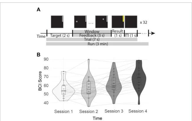
Figure 2. BCI task and performance. (A) Schematic of the BCI task. First the target, a grey bar in the upper or lower portion of the screen, was displayed for 1 s. Next, the subjects have a 3 s feedback period, where the vertical position of the cursor is determined by their neural activity while it moves horizontally at a fixed velocity. This portion corresponds to the analysis window, indicated with a grey bar in the figure. The result is then displayed for 1 s. If the subject reached the target, it will turn yellow; otherwise it will remain grey. There is a 1 s intertrial interval (ITI) between trials where nothing is displayed on the screen. This sequence is repeated 32 times per run, with 6 runs per session. (B) Each subject’s average performance across four days within two weeks. BCI Score is the percentage of correct trials during that session.
2.6. Optimal Control
Our final broad goal was to provide a theoretical explanation for why certain networks support BCI learning. We hypothesized that these regularized net-works might have structures that make it easier for the brain to modulate the patterns of activity that are necessary for BCI control. This hypothesis motiv-ated us to formulate and validate a model to explain how the sparse statistical relationships characteristic of each subgraph could support the production of brain activity patterns implicated in BCI learning [11,
44]. Additionally, this model should account for the brain’s ability to reach these patterns of activity in the context of the BCI task, where there is increased voli-tional modulation of the left motor cortex. Here, we use tools from network control theory to satisfy these conditions [84]. Specifically, we characterize the the-oretical brain activity at each sensor as a vector x(t), and we use the adjacency matrix A of a subgraph to quantify the ease with which that activity can affect other regions. We then incorporate volitional input control as input into the brain (u(t)) at a specific region (given by B). Then, by stipulating
˙
x(t) = Ax(t) + Bu(t), (4)
we model the linear spread of activity along the con-nections in A in the context of input to regions given in B. We note that these dynamics are simple, and
we do not expect them to fully capture the rich-ness of observed signals; nevertheless, simple mod-els have the notable advantages of interpretability and flexibility.
With this model of network dynamics, optimal control trajectories can be formalized and identified by developing a cost function that seeks to minimize two terms: (i) the distance of the current state from the target state and (ii) the energy required for con-trol. Specifically, we solve the following minimization problem: min u ˆ T 0 (xT− x(t))T(xT− x(t)) + ρuκ(t)T uκdt, s.t. x = Ax(t) + Bu(t),˙ x(0) = x0, and
x(T) = xT, (5)
where ρ is a free parameter that weights the input constraint, xT is the target state, and T is the con-trol horizon, which is a free parameter that defines the finite amount of time given to reach the target state. During BCI control, there is specific, targeted control to a specific area of the brain (here, the left motor cortex) in addition to other ongoing control and sensory processes. We wished for our selection of the input matrix B to reflect this richness and also allow for computationally tractable calculations of optimal control, which is difficult for sparse control sets. Therefore, we constructed the input matrix B
so as to allow input that was dominated by the BCI control site, while maintaining minor contributions from other areas. More specifically, rather than being characterized by binary state values, channels other than the one located over left motor cortex were given the smallest non-zeros value that assured low error calculations: approximately 5× 10⁻⁵at their corres-ponding diagonal entry in B. See Supplement for the full derivation from reference [44]. It is important to note that in general the tools from linear con-trol theory are not applicable to the functional net-works commonly derived from neuroimaging data for two reasons. The first reason is that the model which the tools are built upon stipulates a time-dependent propagation of activity along edges; such a propagation is physically true for structural con-nections derived from white matter, but is not gen-erally true for other types of connections used in network models, such as morphometric similarity or most common functional connectivity measures. The second reason is that the model assumes that interac-tions between nodes ‘a’ and ‘c’ are not due to node ‘b’, an assumption that is violated by measures of statist-ical similarity such as the Pearson correlation coeffi-cient which is the measure of functional connectivity most commonly employed in neuroimaging studies. Because we are using neither structural connectivity nor common measures of functional connectivity, it was necessary for us to first prove that the networks we are studying are consistent with our model. To address the first point regarding the propagation of activity along edges, we demonstrate that the struc-ture of the subgraphs used have utility in predicting empirical brain state transitions, and that the relative contribution of each subgraph is related to its tem-poral expression (figure S1C–D). It is only in light of these validations that we are able to interpret our res-ults as a potential model for driving brain activity. To address the second point regarding isolation of pair-wise relations not due to third party effects, we note that the matrix A that we study reflects statistical sim-ilarity in phase after strict regularization that removes redundant statistical relationships (figure S1A–B).
2.6.1. Target state definition
A central hypothesis in this work is that certain reg-ularized subgraphs are better suited to drive the brain to patterns of activity that are beneficial for BCI control than others. To test this hypothesis, we create target states that reflect these beneficial pat-terns, based on previous literature. Target states for motor imagery and attention are obtained for each band individually from references [3, 37, 43], and can be briefly described as follows: α contralateral motor suppression for motor imagery and parietal suppression for attention, β contralateral motor sup-pression and ipsilateral motor activation for motor imagery and vertex suppression for attention, and γ contralateral motor activation for motor imagery
and motor cortex suppression with frontal and occipital activation for attention (figure S10). While acknowledging the limits of anatomical inference from sensor data, we sought to approximate these true functional systems at the sensor level by divid-ing channels into lobes usdivid-ing standard montages provided by Brainstorm [101] software (neuroim-age.usc.edu/brainstorm/Tutorials/MontageEditor). The target state of channels in brain regions where we did not have specific hypotheses for their activ-ity were set to zero; the target state of channels with activation were set to 1 and that of channels with deactivation were set to -1. Initial states were set to 0 for all channels. We then calculate the optimal energy (using the optimal control equation described above) required to reach each of these target states to test the hypothesis that subgraphs that support learning will have lower energy requirements than those that do not.
2.7. Statistical Analyses
Much of our analyses involve testing differences in distributions across subjects for different subgraphs or sessions, both for phase-randomized and empirical data. We also compare these distributions to subject learning rate defined as the slope of performance over time. For the results displayed in figure2here in the main manuscript, we used a repeated meas-ures ANOVA to test for the presence of a main effect across conditions given that the distributions of per-formances were normal (see figure S11). In figure3
here in the main manuscript, we sought to associate learning rate with ranked performance loading. After plotting quantile-quantile plots (see figure S12-S14) for the learning rate, and each of the performance loadings, it became clear that the lowest loadings were not normally distributed. Therefore, we used a linear model combined with non-parametric test-ing utiliztest-ing 5000 permutations (lmPerm package in R https://cran.r-project.org/web/packages/lmPerm). Standardized coefficients were calculated using the lm.beta package in R ( https://cran.r-project.org/web/packages/lm.beta/lm.beta.pdf). We use a Bonferroni correction to control false posit-ive errors due to multiple comparisons across all 6 predictors (α = 0.008). To obtain an estimate of how sensitive our results are to our specific sample, we also plot summary statistics from 500 mod-els obtained from bootstrapping a sample of equal size (N = 60, 3 band and 20 subjects). To exam-ine differences in consistency (figure 4 here in the main manuscript), we use a linear model
(consist-ency ~ band + dataType + rank) to test for a main
effect of data type (null or empirical), band, and sub-graph on consistency (see figure S15). We next sought to determine if different subgraphs had consistently different temporal expression for null and empirical data (figure5here in the main manuscript). We also used a repeated measures ANOVA to test for a main
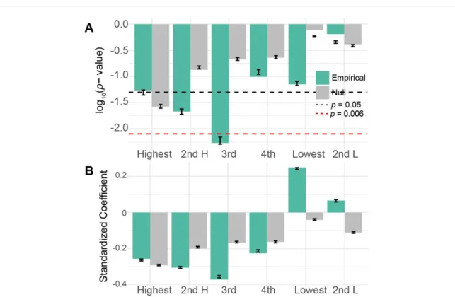
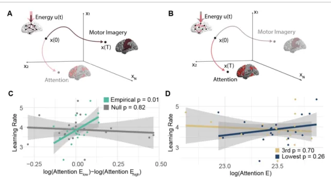
Figure 3. Performance loading is associated with learning. (A) Here we show the p-values for empirical (green) and uniformly phase randomized (grey) data for linear models relating the slope of performance with ranked performance loading from each frequency band. The black line corresponds to p = 0.05, while the red dashed line corresponds to the Bonferroni corrected
α =0.008. Error bars show the standard error and median of p-values from 500 models with bootstrapped samples. (B) The standardized regression coefficients for the same models. Error bars show the standard error and mean of coefficients from 500 models with bootstrapped samples.
effect of subgraph across bands, and paired t-tests to test for differences amongst individual subgraphs (figure S16). Lastly, for the results shown in figure6
here in the main manuscript, we test the relationship between learning rate and optimal control energy dif-ferences for several different models. Pearson’s correl-ations were used, given that the data appears normally distributed and has few outliers (see figure S17-S20). 2.8. Data and Code
Code for analyses unique to this manu-script are available at github.com/jastiso/Net BCI. Code for the NMF algorithm and the NMF parameter selection is available at github. com/akhambhati/Echobase/tree/master/Echobase/ Network/Partitioning/Subgraph. Code for optimal control analyses is available at github.com/jastiso/ NetworkControl. Data necessary to reproduce each figure will be made available upon request.
3. Results
3.1. BCI Learning Performance
Broadly, our goal was to examine the properties of dynamic functional connectivity during BCI learning, and to offer a theoretical explanation for why a certain pattern of connectivity would support individual dif-ferences in learning performance. We hypothesized that decomposing dynamic functional connectivity
into additive N× N subgraphs would reveal unique networks that are well suited to drive the brain to patterns of activity associated with successful BCI control. We use MEG data from 20 healthy adult individuals who learned to control a motor-imagery based BCI over four separate sessions spanning a two week period. Consistent with prior reports of this experiment [24], we find a significant improvement in performance across the four sessions (one-way ANOVA F(3, 57) = 13.8, p = 6.8−7) (figure 2). At the conclusion of training, subjects reached a mean performance of 68%, which is above chance (approx-imately 55 – 60%) level for this task [77].
3.2. Dynamic patterns of functional connectivity supporting performance
To better understand the neural basis of learning performance, we detected and studied the accom-panying patterns of dynamic functional connectiv-ity. First, we calculated single trial phase-based con-nectivity in MEG data in three frequency bands: α (7-14 Hz), β (15-25 Hz), and γ (30-45 Hz). We then used non-negative matrix factorization (NMF) – a matrix decomposition method—to separate the time-varying functional connectivity into a soft par-tition of additive subgraphs. We found that the selec-ted parameters led to an average of 7.4 subgraphs, with a range of 6 to 9, and that all frequency bands had a decomposition error lower than 0.47 (mean
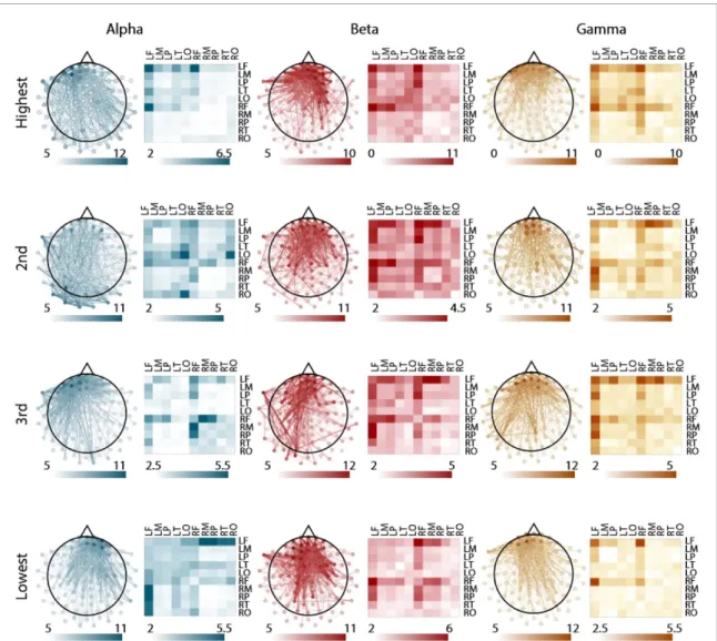
Figure 4. Spatial distribution of subgraph edges that are consistent across participants. Consistent edges for each frequency band and for each ranked subgraph. Left images show individual edges plotted on a topographical map of the brain. Right images show the mean edge weight over sensors for a given region. We studied 10 regions, including the frontal lobe, temporal lobe, parietal lobe, occipital lobe, and motor cortex in both hemispheres. The weight of the edge corresponds to the number of individual participants for whom the edge was among the 25% strongest for that subgraph.
α error = 0.352, mean β error = 0.379, mean γ error = 0.465) (figure S2). The error is the Frobenius norm of the squared difference between our observed and estimated connectivity matrices (with dimen-sions 5152× 384) and takes values between 0 and 1. For each band, the error value is low, giving us con-fidence that we have fairly accurately reconstructed relevant neural dynamics. To determine whether any properties of the identified subgraphs were trivially due to preprocessing choices, NMF parameters, or time-invariant autocorrelation in neural activity, we repeated the full decomposition process after permut-ing the phases of all time series uniformly at random. We found that the statistics of subgraph number and decomposition error were similar for the uniformly phase randomized data, indicating that any differ-ences in subgraph and temporal expression between null and empirical data is not due to the NMF algorithm’s inability to find a good decomposition, but rather due to the structure of the chosen decom-position (figure S2).
We quantified the similarity between each sub-graph’s temporal expression and the time course of performance, and we refer to this quantity as the sub-graph’s performance loading (figure 1). Here, per-formance is calculated as the percentage of accurate trials over a run of 32 trials. We hypothesized that the ranked performance loading would be associated with task learning, as operationalized by the slope of performance over time. It is important to note the distinction between performance and learning: performance is defined as task accuracy and there-fore varies over time, while learning is defined as the linear rate of change in that performance over the course of the experiment (384 trials over 4 days). We tested whether learning was correlated with the performance loading of subgraphs. Because the min-imum number of subgraphs in a given subject was 6, we decided to investigate the top four highest performance loading subgraphs, and the smallest and second smallest nonzero loading subgraphs. We found a general trend that the performance loading
from high loading subgraphs was negatively associ-ated with learning rate, and the performance load-ing from low loadload-ing subgraphs was positively asso-ciated with learning rate (figure3AB). We assessed the statistical significance of these trends and found that only the third highest loading subgraph displayed a performance loading that was significantly correl-ated with learning rate after Bonferroni correction for multiple comparisons (linear model with permuta-tion tests slope ~ loading3 + band : p = 0.005). Per-formance loading from uniformly phase randomized surrogate data for this subgraph was not associated with learning rate (p = 0.292). The direction of the observed effect in the empirical data is notable; sub-jects with lower loading onto high loading subgraphs learned the task better, suggesting that learning is facilitated by a dynamic interplay between several subnetworks. It is also notable that the highest load-ing subgraphs do not have the strongest associations with learning, indicating that the subgraphs that most closely track performance are not the same as the sub-graphs that track changes in performance.
3.3. Spatial properties of dynamic patterns of functional connectivity
Next we sought to better understand why the third highest loading subgraph was most robustly associ-ated with learning. We hypothesized that because of this subgraph’s strong association across subjects, it might recruit sensors near consistent brain regions and reflect the involvement of specific cognitive sys-tems across subjects. To evaluate this hypothesis, we began by investigating the shared spatial prop-erties of this subgraph in comparison to the others. To identify shared spatial features we grouped sub-graphs together by their ranked performance loading, and then quantified how consistent edges were across participants [92] (see Methods). We found that the average consistency varied by frequency band, and differed between the empirical and surrogate data, but not across ranked subgraphs (linear model
con-sistency ~ band + rank + data : Fband(2, 17) = 90.36, pband=9.00× 10⁻¹⁰, Fdata(1, 17) = 41.8, pdata= 5.78× 10⁻⁶). The α band had the most consistent edges, followed by the γ band, and then the β band (tαβ=−12.68, pαβ=4.3× 10⁻¹⁰, tαγ=−10.41, pαγ=1.2× 10⁻⁸). In the uniformly phase random-ized surrogate data, we observed less consistent sub-graphs than those observed in the empirical data
(t =−6.47, p = 5.78 × 10⁻⁶). These observations
support the conclusion that across the population, despite heterogeneous performance, similar regions interact to support performance and learning to vary-ing degrees.
In order to approximate system-level activa-tion with sensor level data, we used lobe montages provided by Brainstorm (see Methods). Subgraphs were dominated by connectivity in the frontal lobe
sensors, with subtle differences in the pattern of con-nections from the frontal lobe sensors to sensors loc-ated in other areas of the brain (figure4). To determ-ine which functional edges were most consistent in each subgraph and frequency band, we calculated the average consistency over each lobe and motor cortex in both hemispheres (for the same analysis in sur-rogate data, see figure S6). In the α band, the most consistent edges on average were located in the left frontal lobe in the highest performance loading sub-graph, in the left occipital lobe in the second highest performance loading subgraph, between right frontal and right motor in the third highest performance loading subgraph, and between left frontal lobe and right parietal lobe in the lowest performance loading subgraph. In the β band, the most consistent edges were located between right and left frontal lobe for the highest and second highest performance loading sub-graph, between left frontal lobe and right motor for the third highest performance loading subgraph, and between left and right frontal lobe for the lowest per-formance loading subgraph. In the γ band, the most consistent edges were located in the left frontal and right frontal lobes for the highest performance load-ing subgraph, in the left frontal lobe and right motor for the second highest performance loading sub-graph, and in left frontal and right frontal lobe for the third highest and lowest performance loading sub-graphs. We wished to demonstrate that the consistent involvement of more frontal sensors across subgraphs was not due to the presence of electro-oculogram (EOG) artifacts that persisted after removal of eye blinks with ICA. We therefore calculated the weighted phase-locking index between both vertical and hori-zontal EOG sensors and all neural sensors. Qualit-atively, we did not observe any consistently strong connectivity between EOG channels and more frontal sensors, indicating that the frontal connectivity iden-tified in our analysis is likely not due to residual arti-facts from eye movements (figure S7). We also note that the most consistent individual edges for each subgraph are still only present in 10−12 individu-als, indicating a high amount of individual variab-ility. Collectively, these observations suggest wide-spread individual variability in the spatial compos-ition of ranked subgraphs, with the most consistent connectivity being located in the frontal lobe during BCI learning.
3.4. Temporal properties of dynamic patterns of functional connectivity
Importantly, subgraphs can be characterized not only by their spatial properties, but also by their temporal expression. We therefore next examined the temporal properties of each subgraph to better understand why the third highest performance loading subgraph was most robustly associated with learning. As a sum-mary marker of temporal expression, we calculated the total energy of the time series operationalized as
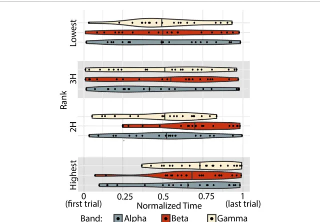
Figure 5. Temporal expression of ranked subgraphs. The peak temporal expression for every subject (black data point), for each frequency band (indicated by color) and for each subgraph (ordered vertically). Violin plots show the density distribution of all subjects’ peaks. The median is marked with a solid line through the violin plot.
the sum of squared values, as well as the time of the peak value of the time series. Across frequency bands, we found no significant dependence between energy and subgraph ranking. We did find a significant effect of rank for the peak time of temporal expression obtained from the empirical data (repeated measures ANOVA peak ~ rank + band : Frank(3, 215) = 6.67, prank=2.53× 10⁻⁴but not from the uniformly phase randomized surrogate data (Frank(3, 215) = 1.28, p = 0.282). Overall, peak times are widely
distrib-uted across individuals. However we find that across bands, the highest performance loading subgraph has a later peak, which is intuitive since performance is generally increasing over time and these subgraphs most strongly track performance.
We then performed post-hoc paired t-tests cor-rected for multiple comparisons (Bonferroni correc-tion α = 0.006) between the highest performance loading subgraph and all other ranked subgraphs in each band. In the α band, the highest performance loading subgraph only peaked significantly later than the lowest (paired t-test N = 20, tlow=8.06, plow= 1.49× 10⁻⁷) after Bonferroni correction (α = 0.006). In the β band, the highest performance loading sub-graph peaked significantly later than all others (paired
t-test N = 20, t2 H=10.9, p2 H=1.39× 10⁻⁹; t3 H=
7.56, p3 H=3.57× 10⁻⁷; tlow=8.07, plow=1.49−7). In the γ band, the highest performance loading subgraph peaked significantly later than the second highest, and lowest loading subgraphs (paired t-test
N = 20, t2 H=4.50, p2 H=2.46× 10⁻⁴; tlow=8.06, plow=1.49× 10⁻⁷) (figure 5). Finally, we asked whether the time of the peak in the third highest performance loading subgraph was associated with learning. We did not find a relationship between peak time and learning in any frequency band (Pear-son’s correlation: α : r = 0.005, p = 0.98, β : r = 0.047,
p = 0.84, γ : r =−0.21, p = 0.37). To summarize these
findings, we note that across participants and espe-cially in the β band, subgraphs that support perform-ance are highly expressed late in learning, when per-formance tends to be highest. However, subgraphs that support learning do not have consistent peaks across subjects, and each individual’s peak does not relate to their learning rate, indicating that some other feature of these subgraphs must explain their role in learning.
3.5. Explaining dynamic patterns of functional connectivity supporting BCI learning via network control theory
Lastly we asked how the third highest loading sub-graph could facilitate successful BCI performance, as shown in figure3. Here, we considered an edge— extracted under penalties of spatial and temporal sparsity—as a potential path for a brain region to affect a change in the activity of another brain region [35,109]. Assuming the true connectivity structure is sparse, the regularization applied in the NMF algorithm can remove large statistical relationships
between regions that are not directly connected, but might receive common input from a third region [28] (see Methods for addition discussion, and see fig-ure S1A–B for the effect of regularization on the pre-valence of triangles). We hypothesized that the pat-tern of edges in this subgraph would facilitate brain states, or patterns of activity, that were predictive of BCI literacy. Specifically, we expected that when the brain mirrored the connectivity of the third sub-graph, the brain could more easily reach states of sustained motor imagery or sustained attention than when the brain mirrored the connectivity of the low-est performance loading subgraph. To operationalize these hypotheses from sensor level data, we identified sensors near motor and attention areas with mont-ages from Brainstorm and set those as targets (see Methods). We also hypothesized that the magnitude of this difference would be associated with each sub-ject’s learning rate. To test these hypotheses, we used mathematical models from network control theory to quantitatively estimate the ease with which the brain can reach a desired pattern of activity given a pat-tern of connectivity (see Methods and figure S1C– D for analyses demonstrating the efficacy of the reg-ularized subgraphs in linearly predicting changes in activity). Specifically we calculated the optimal con-trol energy required to reach a target state (either sus-tained motor imagery or sussus-tained attention) from an initial state when input is applied primarily to the left motor cortex, which was the site of BCI control (fig-ure 6A–B).
We tested whether the third highest performance loading subgraph supported the transition to states of sustained motor imagery or sustained attention with smaller energy requirements than other sub-graphs that did not support learning in the same way. We chose the lowest performance loading subgraph for comparison because it was the only subgraph with a large positive standardized regression coef-ficient for fitting learning, which contrasts sharply with the large negative coefficient for the third sub-graph. For both states (motor imagery and attention), we found no population level differences in energy requirements by the two subgraphs (paired t-test
N = 20, motor imagery: tα=−0.005, pα=0.565,
tβ=1.38, pβ=0.184, tγ=−1.00, pγ=0.329. attention: tα=−1.35, pα=0.193, tβ=−0.344, pβ=0.735, tγ=−0.937, pγ=0.360). We next tested whether the magnitude of the difference in energy required by the two subgraphs to reach a given state tracked with learning rate. In the β band, we observed a significant correlation between the magnitude of the energy difference to reach attentional states and learn-ing rate over subjects (Pearson’s correlation coef-ficient r = 0.560, p = 0.010 3, Bonferroni corrected for multiple comparisons across frequency bands; figure6). Notably, the relationship remained signi-ficant when controlling for subgraph density (linear model slope∼ energy_difference + density_difference:
tenergy=2.68, penergy=0.015 8, tdensity=−0.266, pdensity=0.794). When using subgraphs derived from the uniformly phase randomized surrogate data, the relationship was not observed (Pearson’s correlation
r =−0.056 8, p = 0.819). We next asked which
sub-graph contributed most to this effect. We found no significant relationship between learning rate and the energy required to reach the attentional state by the third highest performance loading subgraph (Pearson’s correlation r =−0.389, p = 0.702) or by the lowest performance loading subgraph (Pearson’s correlation r = 0.227, p = 0.335). This finding sug-gests that learning rate depends on the relative dif-ferences between subgraphs, rather than the energy conserving architecture of one alone. As a final test of specificity, we assessed whether this difference was selective to the third highest and lowest perform-ance loading subgraph. We found no significant rela-tionship when testing the difference of the highest with the third highest performance loading subgraph (Pearson’s correlation r =−0.554, p = 0.586), the highest with the lowest performance loading sub-graph (Pearson’s correlation r = 0.40, p = 0.077), the second highest with the third highest performance loading subgraph (Pearson’s correlation r = 0.266,
p = 0.257), or the second highest with the lowest
per-formance loading subgraph (Pearson’s correlation
r =−0.072, p = 0.764). This pattern of null results
underscores the specificity of our finding.
3.6. Reliability and specificity of inferences from network control theory
Collectively, our findings are consistent with the hypothesis that during BCI learning, one subnetwork of neural activity arises, separates from other ongo-ing processes, and facilitates sustained attention. An alternative hypothesis is that our results are due to trivial factors related to the magnitude of the atten-tional state, or could have just as easily been found if we had placed input to a randomly chosen region of the brain, rather than to the left motor cortex which was the actual site of the BCI control. To determine whether these less interesting factors could explain our results, we performed the same network control calculation but with a spatially non-overlapping tar-get state, and then—in a separate simulation—with a mirrored input region (right motor cortex rather than left motor cortex). We performed the spatial shifting by ordering the nodes anatomically (to pre-serve spatial contiguity), and then circularly shift-ing the attention target state by a random number between 1 and N− 1. For 500 circularly shifted states, only 3 (0.6%) had a correlation value equal to or stronger than the one observed (figure S8). Further-more, we found no significant relationship between learning rate and the difference in energy required by the two subgraphs to reach the true attention state when input was applied to the right motor cortex
Figure 6. Separation of the ability to modulate attention is associated with learning. Different patterns of connections will facilitate transitions to different patterns of brain activity. We hypothesize that the ease with which connections in certain regularized subgraphs facilitate transitions to patterns of activity that support either motor imagery (A) or attention (B) will be associated with learning rate. We use network control theory to test this hypothesis. We model how much energy (u(t)) is required to navigate through state space from some initial pattern of activity x(0) to a final pattern of activity x(T). Some networks (e.g. the brown network in panel A) will require very little energy (schematized here with a smaller, solid colored arrow) to reach patterns that support motor imagery, while other networks (e.g. the pink network in panel B) will have small energy requirement to reach patterns of activity that support attention. (C) The relationship between learning rate and the difference in energy required to reach the attention state when the underlying network takes the form of the lowest versus third highest performance loading subgraphs for empirical data (green) and uniformly phase randomized surrogate data (grey). (D) The relationship between the learning rate and the energy required to reach the attention state when the underlying network takes the form of the lowest performance loading subgraph, or when the underlying network takes the form of the third highest
performance loading subgraph.
instead of the left motor cortex (Pearson’s correla-tion t = 0.711, p = 0.313). Together, these two find-ings suggest that the relationship identified is specific to BCI control.
Finally, we assessed the robustness of our res-ults to choices in modeling parameters. First we per-formed the computational modeling with two differ-ent sets of control parameter values (see Supplemdiffer-ent). In both cases, the significant relationship remained between learning rate and the difference in energy required by the two subgraphs to reach the atten-tional state (set one Pearson’s correlation coefficient
r = 0.476, p = 0.033 8; set two Pearson’s correlation
coefficient r = 0.514, p = 0.020 4). Second, since our target states were defined from prior literature, there was some flexibility in stipulating features of those states. To ensure that our results were not unduly influenced by these choices, we tested whether ideo-logically similar states would provide similar results. Namely, we assessed (i) the impact of varying the magnitude of (de)activation by changing )1 to (-)2, (ii) the impact of the neutral state by changing 0 to 1, and (iii) the impact of negative states by chan-ging -1, 0 and 1 to 1, 2, and 3. We found a con-sistent relationship between learning rate and the difference in energy required by the two subgraphs to reach the attentional state when we changed the magnitude of activation/deactivation (Pearson’s
correlation coefficient r = 0.560, p = 0.010 3), as well as when we changed the neutral state (Pearson’s correlation coefficient r = 0.520, p = 0.018 8). How-ever, we found no significant relationship when removing negative states (Pearson’s correlation coef-ficient r = 0.350, p = 0.130), indicating that this result is dependent on our choice to operationalize deactiv-ation as a negative state value. After performing these robustness checks, we conclude that a selective sep-aration of the third highest and lowest performance loading subgraphs impacts their ability to drive the brain to patterns of sustained attention in the β band in the context of BCI control. This result is robust to most of our parameter choices, is selective for biolo-gically observed states, and is not observed in surrog-ate data.
4. Discussion
In this work, we use a minimally constrained decom-position of dynamic functional connectivity during BCI learning to investigate which groups of phase locked brain regions (subgraphs) support BCI con-trol. The performance loading onto these subgraphs favors the theory that dynamic involvement of sev-eral subgraphs during learning supports successful control, rather than extremely strong expression of a
single subgraph. Additionally, we find a unique asso-ciation for the third highest loading subgraph with learning at the population level. This result shows that learning is not simply explained by the subset of edges that has the most similar temporal expression to behavior, but rather that a subnetwork with a mid-dling range of similarity has the strongest relation-ship with performance improvement. While the spa-tiotemporal distribution of this subgraph was vari-able across individuals, we did observe some consist-encies at the group level. Spatially, the third highest loading subgraph showed strong edges between left frontal and right motor cortices for low frequencies, and left frontal and left motor cortices for the γ band. Lower frequencies showed stronger connectivity to the ipsilateral (to imagined movement) motor cortex, suggesting a possible role in suppression for select-ive control. This subgraph also showed the highest expression earlier than the other ranked subgraphs we investigated, perhaps linking it to the transition from volitional to automatic control.
We next wished to posit a theory of how these sub-graphs fit with previously identified neural processes important for learning, despite their heterogeneity across subjects. After quantifying the extent to which NMF regularization removed potentially redundant relationships between regions (figure S1A–B), we suggested that the regularized pattern of statistical relationships identified in this subgraph could com-prise an avenue through which brain activity could be modulated via cognitive control or external input. We then hypothesized that these networks would be better suited to modulate activity in either regions implicated in attention or in motor imagery than other subgraphs, and further that individuals whose networks better modulated activity in these regions would display greater task learning [56]. We chose to operationalize the ‘ease of modulation’ with a met-ric from network control theory called optimal control
energy. Optimal control energy quantifies the
min-imum input needed to drive the brain from an initial pattern of activity to a final pattern of activity, while also assuring that the pattern of activity stays close to the target state at every point in time. This last con-straint ensures that we are unlikely to pass through biologically unfeasible patterns of activity. The notion of optimal control energy that we use here assumes a particular linear model of how neural dynamics change given potential avenues of communication between regions. Importantly, in the supplement (fig-ure S1C–D (stacks.iop.org/JNE/17/046018/mmedia)) we show that our subgraphs predict empirical brain state changes according to this model, and that the contribution of each subgraph to empirical changes in brain state is related to its temporal expres-sion. Using this model, we did not find any pop-ulation differences in optimal control energy when the simulation was enacted on the third highest performance loading subgraph compared to the
lowest performance loading subgraph. However, we did find that the magnitude of this difference was associated with learning in individual subjects. This result was specific to the β band and to brain regions implicated in attention. Critically, the relation to learning could not be explained by the energy of either subgraph alone, was not present in surrogate data derived from a uniformly phase randomize null model, and was robust to parameter choices. Over-all, the observations support our hypothesis that in the β band the subgraphs we identified that support learning are well suited to modulate activity in brain regions associated with attention.
4.1. A delicate balance of interactions is required for BCI learning
Our initial analysis explored the relationship between performance loading and learning. It is important to note the behavioral difference between perform-ance and learning: we use the term performperform-ance to refer to task accuracy over time, whereas we use the term learning to refer to how well a subject is able to increase that accuracy. With that distinction in mind, we aimed to better understand how subgraphs that vary similarly to performance (those with high performance loading) relate to learning. We found that the subgraph with the third highest performance loading was most strongly associated with learning and that a narrow distribution of performance load-ing across all subgraphs was associated with better learning. Together, these two observations are in line with previous research in motor and spatial learning, which shows that some brain structures display dif-ferential activity during learning that is independent of performance [86,95]. Our work adds to this lit-erature by demonstrating that in addition to targeted differences in individual brain regions or networks, a minimally constrained decomposition of dynamic functional connectivity across the whole brain reveals that separable processes are most associated with per-formance and with learning.
Additionally, we find that BCI learning is not explained simply by the processes most strongly asso-ciated with performance and learning individually, but by a distributed loading across many different subgraphs. This notion is supported by the sign of the beta value for ranked subgraphs. Generally, sub-graphs with higher ranked loading were negative betas, while subgraphs with lower ranked loading were positive betas. A wealth of whole brain con-nectivity analyses have similarly shown that the inter-action between systems is an important component of skill learning specifically, and other domains of learn-ing more generally [2,8]. While we observed marked interactions between many regions, the majority were located in the frontal lobe for all frequency bands. Even for α and β frequencies in the highest loading subgraph, we see involvment of frontal regions and