arXiv:1004.0836v1 [astro-ph.EP] 6 Apr 2010
THE THERMAL EMISSION OF THE EXOPLANETS WASP-1b AND WASP-2b
PETERJ. WHEATLEY1, ANDREWCOLLIERCAMERON2, JOSEPHHARRINGTON3, JONATHANJ. FORTNEY4, JAMESM. SIMPSON2, DAVIDR. ANDERSON5, ALEXISM. S. SMITH5, SUZANNEAIGRAIN6, WILLIAMI. CLARKSON7, MICHAËLGILLON8,9, CAROLEA. HASWELL10, LESLIEHEBB11, GUILLAUMEHÉBRARD12, COELHELLIER5, SIMONT. HODGKIN13, KEITHD. HORNE2, STEPHENR. KANE14, PIERREF. L. MAXTED5, ANDREWJ. NORTON10, DONL. POLLACCO15, FREDERICPONT16, IANSKILLEN17,
BARRYSMALLEY5, RACHELA. STREET18, STEPHANEUDRY8, RICHARDG. WEST19, DAVIDM. WILSON5,
1Department of Physics, University of Warwick, Coventry CV4 7AL, UK
2School of Physics and Astronomy, University of St Andrews, North Haugh, St Andrews, Fife KY16 9SS, UK 3Department of Physics, University of Central Florida, Orlando, FL 32816-2385, USA
4Department of Astronomy and Astrophysics, University of California, Santa Cruz, CA 95064, USA 5Astrophysics Group, School of Chemistry and Physics, Keele University, Staffordshire, ST5 5BG, UK 6Department of Physics, University of Oxford, Denys Wilkinson Building, Keble Road, Oxford OX1 3RH, UK
7STScI, 3700 San Martin Drive, Baltimore, MD 21218, USA
8Observatoire de Genève, Université de Genève, 51 Ch. des Maillettes, 1290 Sauverny, Switzerland 9Institut d’Astrophysique et de Géophysique, Université de Liège, Allée du 6 Août, 17, Bat. B5C, Liège 1, Belgium
10Department of Physics and Astronomy, The Open University, Milton Keynes, MK7 6AA, UK 11Department of Physics and Astronomy, Vanderbilt University, Nashville, TN 37235, USA
12Institut d’Astrophysique de Paris, UMR7095 CNRS, Université Pierre & Marie Curie, 98bis boulevard Arago, 75014 Paris, France 13Institute of Astronomy, Madingley Road, Cambridge CB3 0HA, UK
14Michelson Science Center, Caltech, MS 100-22, 770 South Wilson Avenue, Pasadena, CA 91125, USA
15Astrophysics Research Centre, School of Mathematics & Physics, Queen’s University, University Road, Belfast, BT7 1NN, UK 16School of Physics, University of Exeter, Exeter, EX4 4QL, UK
17Isaac Newton Group of Telescopes, Apartado de Correos 321, E-38700 Santa Cruz de la Palma, Tenerife, Spain 18Las Cumbres Observatory, 6740 Cortona Dr. Suite 102, Santa Barbara, CA 93117, USA
19Department of Physics and Astronomy, University of Leicester, Leicester, LE1 7RH, UK Draft version April 7, 2010
ABSTRACT
We present a comparative study of the thermal emission of the transiting exoplanets 1b and WASP-2b using the Spitzer Space Telescope. The two planets have very similar masses but suffer different levels of irradiation and are predicted to fall either side of a sharp transition between planets with and without hot strato-spheres. WASP-1b is one of the most highly irradiated planets studied to date. We measure planet/star contrast ratios in all four of the IRAC bands for both planets (3.6–8.0µm), and our results indicate the presence of a
strong temperature inversion in the atmosphere of WASP-1b, particularly apparent at 8µm, and no inversion in
WASP-2b. In both cases the measured eclipse depths favor models in which incident energy is not redistributed efficiently from the day side to the night side of the planet. We fit the Spitzer light curves simultaneously with the best available radial velocity curves and transit photometry in order to provide updated measurements of system parameters. We do not find significant eccentricity in the orbit of either planet, suggesting that the inflated radius of WASP-1b is unlikely to be the result of tidal heating. Finally, by plotting ratios of secondary eclipse depths at 8µm and 4.5 µm against irradiation for all available planets, we find evidence for a sharp
transition in the emission spectra of hot Jupiters at an irradiation level of 2× 10⁹erg s−1cm−2. We suggest
this transition may be due to the presence of TiO in the upper atmospheres of the most strongly irradiated hot Jupiters.
Subject headings:
1. INTRODUCTION
The Spitzer Space Telescope (Werner et al. 2004) has been used to carry out the first photometry and emis-sion spectroscopy of exoplanets that orbit main se-quence stars (Deming et al. 2005; Charbonneau et al. 2005; Richardson et al. 2007; Grillmair et al. 2007). This was achieved by observing transiting planets at secondary eclipse (when the planet is eclipsed by the star) which allows the emission of the planet to be separated from that of the star. Photometry and spectroscopy are the key measurements needed to determine the physical properties of any astronom-ical object, and secondary eclipse observations allow us to consider the temperature structure and chemical
tion of exoplanet atmospheres and the redistribution of en-ergy from the day side to the night side of the planet (e.g. Burrows et al. 2005; Fortney et al. 2005; Seager et al. 2005; Barman et al. 2005).
Secondary eclipse detections have been made from the ground (e.g. de Mooij & Snellen 2009; Sing & López-Morales 2009) but since the signal is weak even in the best cases (of order 0.1 per cent in hot Jupiters) the bulk of measurements to date are from space. Together with detections in the optical with CoRoT and
Kepler (Snellen et al. 2009; Alonso et al. 2009; Borucki et al.
2009) and the near infrared with HST (Swain et al. 2009a,b),
Spitzer is providing an increasingly clear picture of the
thermal emission of exoplanets.
but fortunately this is a range in which strong molecular bands are expected, providing good constraints on atmospheric con-ditions. The IRAC observing modes also allow more efficient observations of these fainter systems, to some extent compen-sating for their lower brightness. The rapidly growing number of moderately-bright transiting hot Jupiters therefore provide an excellent opportunity to improve our understanding of ex-oplanet atmospheres.
The existing Spitzer observations show that hot Jupiters are strongly heated by their parent stars, with typical bright-ness temperatures in the range 1000–2000 K, and that their spectra deviate strongly from black bodies. Preliminary the-oretical calculations predicted strong molecular absorption in the IRAC bands (Burrows et al. 2005; Fortney et al. 2005; Seager et al. 2005; Barman et al. 2005), for which there is ev-idence in some systems (e.g. HD189733b; Charbonneau et al. 2008), however other systems have measured brightness tem-peratures in excess of expectations, indicating emission fea-tures in the IRAC bands (e.g. HD209458b; Knutson et al. 2008). In these cases it is thought that an opacity source high in the atmosphere results in a hot stratosphere and that the molecular bands are driven into emission by the tem-perature inversion (Hubeny et al. 2003; Fortney et al. 2006; Harrington et al. 2007; Burrows et al. 2007; Sing et al. 2008). Fortney et al. (2008) and Burrows et al. (2008) suggest that ir-radiated exoplanets may fall into two distinct classes, those with and those without hot stratospheres, depending on the level of incident stellar flux (dubbed pM and pL class planets respectively by Fortney et al. 2008). The bright-est and bbright-est studied systems, HD209458b and HD189733b, fall either side of the predicted transition between these classes (Fortney et al. 2008), and their IRAC fluxes sup-port the presence of a hot stratosphere in HD209458b (Burrows et al. 2007; Knutson et al. 2008) and its absence in HD189733b (Charbonneau et al. 2008). Most of the other systems that have been observed in all four IRAC bands also seem to support this overall picture (Knutson et al. 2009; Machalek et al. 2009; Todorov et al. 2010; O’Donovan et al. 2010; Machalek et al. 2010; Campo et al. 2010), but XO-1b and TrES-3 do not, with XO-1b presenting evidence for a temperature inversion despite low irradiation (Machalek et al. 2008, 2009), and TrES-3 not exhibiting evidence for a temper-ature inversion despite high irradiation (Fressin et al. 2010). It may be that additional parameters dictate the presence of a temperature inversion, although to some extent the picture is confused by the different models and criteria for inversion de-tection applied by different authors. Gillon et al. (2010) show that the planets studied to date cover a wide region in color-color space, and do not fall clearly into two groups.
In this paper we present Spitzer IRAC secondary eclipse
parative study since they have near identical mass (0.9 MJ)
and yet WASP-1b is highly irradiated and expected to have a hot stratosphere, while WASP-2b is not (Fortney et al. 2008). Indeed, WASP-1b is one of the most highly irra-diated planets studied with Spitzer to date (incident flux of 2.5 × 10⁹erg s−1cm−2). It is also one of the group of oversized
hot Jupiters that have radii larger than can be explained with canonical models (Charbonneau et al. 2007).
In addition to presenting and discussing Spitzer detections of WASP-1b and WASP-2b, we present revised parameters for both planets based on simultaneous fits of all available photometry and spectroscopy.
2. OBSERVATIONS
2.1. Spitzer secondary-eclipse observations
The Spitzer IRAC instrument provides images of two adja-cent fields, each in two wavebands (one field at 3.6 & 5.8µm,
the other at 4.5 & 8.0µm; Fazio et al. 2004). We observed the
expected times of two secondary eclipses for each of WASP-1b and WASP-2b, allowing us to cover all four wavebands without repointing the telescope during an observation. A log of our four observations is given in Table 1.
The precise target positions were carefully chosen in order to avoid bad pixels, keep saturated stars off of the array, ex-clude bright stars from regions known to scatter light onto the IRAC detectors, and to place bright comparison stars on the detector (although these were not used in our final analysis). The pointing position was not dithered during the observa-tions.
Our observations were made in full array mode with 12 s frame times (10.4 s effective exposure), except for the 3.6/5.8µm observation of WASP-2b, which was made in
stel-lar photometry mode with pairs of 2 s frames taken in the
3.6µm band for each 12 s frame in the 5.8 µm band. This
mode was used in order to avoid saturating the target in the 3.6µm band. Observation durations are listed in
Ta-ble 1 and were chosen in order to cover approximately twice the expected secondary eclipse duration (transit durations are 3.7 h and 1.8 h for WASP-1b and WASP-2b respectively; Charbonneau et al. 2007).
2.2. Radial velocity and transit observations
In addition to the Spitzer secondary eclipse observations we also re-analyzed radial-velocity measurements of WASP-1 and WASP-2 from Collier Cameron et al. (2007b) and z-band primary transit observations from Charbonneau et al. (2007) as well as the SuperWASP discovery photometry from Collier Cameron et al. (2007b).
For WASP-1 we also included the I-band transit observa-tions of Shporer et al. (2007) in our analysis.
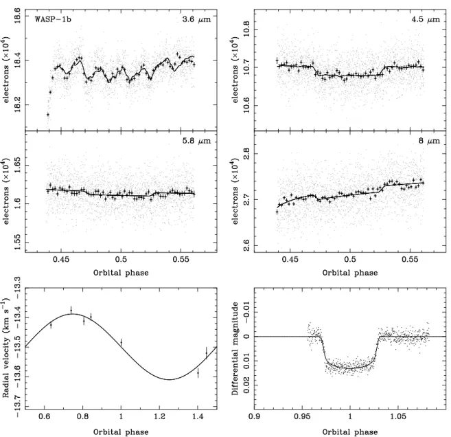
Figure 1. Upper panels show the Spitzer IRAC light curves of the star WASP-1 during the expected times of secondary eclipse of the planet WASP-1b. Points
show the measurements from individual images, crosses show the data binned into five hundred bins per orbital period. Solid lines show our best fits to the eclipse light curves, including linear decorrelation and other instrumental effects described in Sects. 4.1 & 4.2. The lower panels show the radial velocity curve of WASP-1 (measured with SOPHIE at OHP) and the z-band optical light curve during primary transit (from Keplercam), each plotted on different phase ranges. These data were fitted simultaneously with the secondary eclipse observations.
For WASP-2 we included additional radial-velocity mea-surements made with the Swiss 1.2-m Euler telescope at La Silla, Chile between 2008 October 14 and November 6, and six pairs of measurements made with HARPS on the ESO 3.6-m telescope at La Silla on the nights of 2008 October 14/15, 15/16 and 16/17.
All the radial-velocity measurements used in our analy-sis are plotted in the lower-left panels of Figs. 1 & 2. Pri-mary transit photometry is shown in the lower-right panels of these figures, but we only plot the transit photometry from Charbonneau et al. (2007) for clarity.
3. Spitzer DATA REDUCTION
For our analysis we used the Basic Calibrated Data (BCD) files generated by the IRAC pipeline.1One image is produced
for each exposure, with the processing including: dark current 1Pipeline description document: http://ssc.spitzer.caltech.edu/irac/dh/PDD.pdf
and bias subtraction; muxbleed correction for the InSb arrays; non-linearity correction; scattered light subtraction; flat field-ing; and photometric calibration. The pipeline version used to process each observation is given in Table 1.
We first renormalized each BCD image into units of elec-trons by multiplying by exposure time and detector gain and dividing by the flux conversion factor given in the BCD file headers.
Light curves were extracted using simple aperture photom-etry with a source aperture radius of four pixels in all bands. The aperture position was centred on the target in each image by centroiding the x and y pixel positions within a 9 pix search box. The background contribution was estimated by calcu-lating the mode of pixel values in an annulus centred on the source with inner and outer radii of 8 and 20 pixels. Uncer-tainties were estimated using counting statistics normalised to the measured variance in the background in each image.
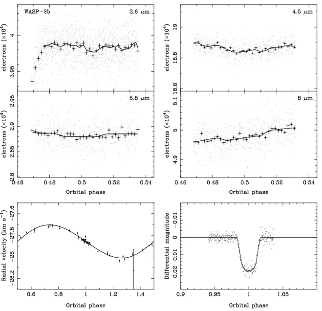
Figure 2. Upper panels show the Spitzer IRAC light curves of the star WASP-2 during the expected times of secondary eclipse of the planet WASP-2b. Points
show the measurements from individual images, crosses show the data binned into five hundred bins per orbital period. Solid lines show our best fits to the eclipse light curves, including linear decorrelation and other instrumental effects described in Sects. 4.1 & 4.2. The lower panels show the radial velocity curve of WASP-2 (measured with SOPHIE, Coralie and HARPS) and the z-band optical light curve during primary transit (from Keplercam), each plotted on different phase ranges. These data were fitted simultaneously with the secondary eclipse observations.
radiation hits we adopted a two stage process in which we first rejected images for which photometric measurements were extreme outliers from the mean of the entire dataset
(> 10σ). We then formed a running mean of the remaining
measurements across one hundred images and rejected im-ages that were highly significant outliers from the running mean (> 5σ). In total, 311 of 12,806 images were rejected (2
per cent). The proportion of frames rejected from each light curve is given in Table 2.
The UTC times from the image headers were corrected to the Solar System barycenter using our own code and the co-ordinates of the Spitzer spacecraft from the HORIZONS on-line ephemeris system of the Jet Propulsion Laboratory.2The
corrections applied to each observation are listed in Table 1. The maximum change in correction during an observation was 2 s, and so it was sufficient only to apply a single
aver-2http://ssd.jpl.nasa.gov/horizons.cgi
age offset to each observation.
The resulting Spitzer light curves are plotted in Figs. 1 & 2. The light curves were fitted at full resolution (described in the following section), but they are plotted here also binned into five hundred phase bins for clarity.
4. LIGHT CURVE DECORRELATION AND PARAMETER FITTING 4.1. 3.6 and 4.5µm decorrelation
All four IRAC detectors exhibit distinctive patterns of cor-related systematic error. Data from the 3.6 µm and 4.5 µm (InSb) detectors are most strongly affected by
intra-pixel variations in quantum efficiency (Reach et al. 2005; Charbonneau et al. 2005; Morales-Calderón et al. 2006). While the impact of these sensitivity differences is mini-mized by not moving the pointing during an observation, the spacecraft pointing tends to oscillate around the nominal posi-tion, with an amplitude of around 0.1 pix, leading to position-dependent variations in the measured stellar flux. The effect
Figure 3. Geometry of partial eclipse phases, showing the angles α and β used in computing the visible fraction η of the planetary disc. For illustrative clarity
only, the planet is shown in front of the star.
Table 2
Target pixel positions and fractions of rejected images for each of our Spitzer IRAC light curves. The pixel ranges correspond to the full range of
the Gaussian-filtered positions used for decorrelation in Sect. 4.1.
Target Band x pixel y pixel rejected
µm median range median range %
WASP-1b 3.6 192.14 0.15 152.44 0.22 2.1 4.5 187.14 0.15 94.72 0.21 1.8 5.8 185.51 153.57 3.5 8.0 186.26 94.09 3.7 WASP-2b 3.6 203.81 0.06 149.78 0.16 0.3 4.5 107.37 0.05 155.02 0.10 2.6 5.8 197.19 151.04 3.3 8.0 106.22 153.21 2.5
can be seen clearly in the 3.6µm light curve of WASP-1b (top
left panel of Fig. 1). Knutson et al. (2008) modelled these sys-tematics using a two-dimensional polynomial fit to the instan-taneous pointing offset from the centre of the pixel on which the stellar image was centred. For observations in which the pointing was changed during an observation it was found that a quadratic function was needed to remove this intra-pixel ef-fect (Knutson et al. 2008; Charbonneau et al. 2008). For ob-servations where the pointing position is not changed (like our own) some authors find acceptable fits using just a linear func-tion of pixel posifunc-tion (Knutson et al. 2009; Machalek et al. 2009; Fressin et al. 2010).
For our analysis we tried both quadratic and linear decorre-lation functions, similar to those of Knutson et al. (2008) and Knutson et al. (2009). The quadratic function is
p′= 1+c
x(x−x0)+cxx(x−x0)2+cy(y−y0)+cyy(y−y0)2+ctt (1)
where (x, y) are the instantaneous coordinates of the stellar
image, (x0, y0) are the coordinates of the centre of the
fidu-cial pixel, and t is the mid-time of the exposure. The last term allows for a linear trend in the light curves as noted by Knutson et al. (2009). The linear decorrelation function is the same as Eqn. 1, except that the constants cxxand cyywere set
to zero. The measured target positions were first smoothed us-ing a movus-ing Gaussian filter with a width of 12 observations. The median pixel positions and pixel ranges for each of our observations are given in Table 2.
Despite the use of these decorrelation functions, we were unable to find acceptable fits when including the steep in-crease in flux seen at the beginning of the 3.6µm light curves
of both planets (Figs. 1 & 2). Inspection of the corre-sponding background light curves revealed variations simi-lar to that noted by Knutson et al. (2009) and attributed to an illumination-dependent sensitivity effect similar to that seen in the 5.8 and 8.0µm detectors (see Sect. 4.2). For the fits
presented in this paper we decided to exclude the first 30 min and 21 min respectively of the 3.6µm light curves of
WASP-1b and WASP-2b.
4.2. 5.8 and 8.0µm detrending
The 5.6µm and 8.0 µm (Si:As) detectors suffer from
time-dependent sensitivity variations that depend on the recent illu-mination history of each pixel (Knutson et al. 2007). This can be seen clearly in the 8µm light curves of both WASP-1b and
WASP-2b (Figs. 1 & 2). Again we followed the methodology of Knutson et al. (2008) in fitting a quadratic ramp function in logarithmic time, of the form
p′= 1+ctτ+cttτ2, (2)
whereτ = ln(t−t0), t being the mid-time of the exposure and
t0 being a fiducial time 30 minutes prior to the first exposure
of the observing sequence.
4.3. Secondary eclipse profile
The secondary eclipse profile is computed assuming the planet’s day-side hemisphere to have a uniform surface bright-ness, and a star/planet flux ratio f = Fp/F∗.
Given the ratio p = Rp/R∗ of the planetary to the stellar radius, and a dimensionless separation z in units of the stellar radius, the planet is partially eclipsed when 1−p< z < 1+p.
At such times, the visible fraction of the planet’s disk is given by
η(p, z) =β−cosβ sin β+(α−cosα sin α)/p 2 π (3) where cosα =1−p 2+z2 2z (4) and cosβ =1−p 2−z2 2pz , (5)
using the geometry sketched in Fig. 3. Outside transit, when
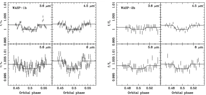
Figure 4. Spitzer IRAC light curves covering the secondary eclipses of the exoplanets WASP-1b and WASP-2b. Instrumental effects modelled in our fitting
process have been removed and the light curves have been scaled to the flux of the star in each band. The light curves have been binned into five hundred phase bins per orbital period.
Figure 5. The 3.6 µm light curve of WASP-1b fitted using the quadratic
decorrelation function described in Sect. 4.1. The data have been binned into five hundred phase bins per orbital period. Instrumental effects have been removed in the bottom panel.
When z< 1−p, the planet is totally eclipsed andη = 0. At
any time, the total observed flux from the star and planet is
F = F∗(1+fη(p, z)).
4.4. Parameter fitting
We solved for the full set of orbital and photometric param-eters using the Markov-chain Monte-Carlo (MCMC) code de-scribed by Collier Cameron et al. (2007a) and Pollacco et al. (2008), modified to incorporate the secondary-eclipse and decorrelation models described in Sects. 4.1–4.3.
At each step in the Markov chain, synthetic optical light curves and radial-velocity curves are computed using the methodology described by Pollacco et al. (2008), using the first nine parameters listed in Table 3. This particular set of parameters is chosen for their mutual near-orthogonality, as described by Ford (2005) and Collier Cameron et al. (2007a). The secondary eclipse models for the four IRAC detectors are computed as described in Sect. 4.3, multiplying the trial value
of the planet/star flux ratios f in each bandpass by the planet visibility functionη at each time of observation. The
normal-ized light curve (1+fη) is then co-multiplied by the
appro-priate sub-pixel (Eqn. 1) or ramp (Eqn. 2) sensitivity model with a trial set of model coefficients {cx, cy, ct} (for linear
decorrelation in the 3.6 & 4.5µm bands), {cx, cxx, cy, cyy, ct}
(for quadratic decorrelation), or{ct, ctt} (in the 5.8 & 8.0 µm
bands) for each detector in turn.
The normalized model light curve thus has the form
p = (1+fη)(1+cx(x−x0)+cy(y−y0)+ctt) (6)
for linear decorrelation of the 3.6µm and 4.5 µm light curves, p = (1+fη)(1+cx(x−x0)+cxx(x−x0)2+cy(y−y0)+cyy(y−y0)2+ctt)
(7) for quadratic decorrelation of the 3.6µm and 4.5 µm
detec-tors, and
p = (1+fη)(1+ctτ+cttτ2) (8)
for the 5.8µm and 8.0 µm light curves.
The observed fluxes di and the normalized model data pi are orthogonalized by subtracting their respective inverse
variance-weighted mean values ˆd and p, then computing theˆ
inverse variance-weighted scale factor
F∗=X i (di−d)(pˆ i−p)wˆ i/ X i (pi−p)ˆ2wi. (9)
where the weights wi= 1/Var(di) are the inverse variances
as-sociated with the observed fluxes. The logarithmic likelihood of obtaining the observed data given the model is quantified by χ2 Spitzer= X i wi(di−dˆ−F∗(pi−p))ˆ 2. (10)
This contribution is added to theχ2statistic computed for the
photometric and radial-velocity data. This is described in de-tail by Pollacco et al. (2008), to which the reader is referred.
At each step in the MCMC calculation, the planet/star flux ratios in the four IRAC bands and the nine other model pa-rameters {T0, P,tT, ∆F,b,K,e cosω,e sin ω} are each given a
Table 3
Proposal parameter values derived from MCMC parameter fitting to combined optical light curves, radial-velocity curves and Spitzer secondary-eclipse data.
Parameter Symbol WASP-1b WASP-2b Units
linear decor. quadratic decor. linear decor.
BJD of primary mid-transit T0 2453998.1924 ± 0.0002 2453998.1924 ± 0.0002 2454002.2754 ± 0.0002 d
Orbital period P 2.519954 ± 0.000006 2.519959 ± 0.000006 2.152225 ± 0.000003 d
Eclipse duration tT 0.1550 ± 0.0006 0.1550 ± 0.0006 0.0752 ± 0.0009 d
Planet/star area ratio ∆F 0.0101 ± 0.0001 0.0101 ± 0.0001 0.0178 ± 0.0004
Impact parameter b 0.064+0.048 −0.042 0.044−+00.052.030 0.731+−00.018.022 Stellar mass M∗ 1.217 ± 0.015 1.216 ± 0.015 0.861 ± 0.022 M⊙ Stellar RV amplitude K 0.111 ± 0.010 0.111 ± 0.009 0.154 ± 0.004 km s−1 e cos ω −0.0026 ± 0.0007 −0.0012 ± 0.0007 −0.0013 ± 0.0009 e sin ω −0.0053 ± 0.0076 −0.0083 ± 0.0073 −0.048 ± 0.021 Flux ratio at 3.6 µm f3.6 0.00184 ± 0.00016 0.00117 ± 0.00016 0.00083 ± 0.00035 Flux ratio at 4.5 µm f4.5 0.00217 ± 0.00017 0.00212 ± 0.00021 0.00169 ± 0.00017 Flux ratio at 5.8 µm f5.8 0.00274 ± 0.00058 0.00282 ± 0.00060 0.00192 ± 0.00077 Flux ratio at 8.0 µm f8.0 0.00474 ± 0.00046 0.00470 ± 0.00046 0.00285 ± 0.00059
random Gaussian perturbation, with a "jump length" of or-der the uncertainty in the fitting parameter concerned. The Spitzer secondary-eclipse data are then divided by the scaled model secondary-eclipse profile, and the parameters of the decorrelation function are fitted by linear least-squares, using singular-value decomposition (Press et al. 1993). The proce-dure is the same as that used by Gillon et al. (2010). The model data are computed and fitted to the observations, and the globalχ2 statistic is computed. A decision is then made
to either accept or reject the proposed parameter set accord-ing to the Metropolis-Hastaccord-ings algorithm: ifχ2has decreased,
the step is accepted unconditionally. Ifχ2has increased by an
amount∆χ2, the proposal may be accepted with probability
exp(−∆χ2/2).
For the first few hundred steps of a typical run, the param-eter values evolve in a way that drivesχ2 down to a global
minimum value. The algorithm then explores the joint poste-rior probability distribution of the parameters in the neigh-borhood of the optimal solution. We use the approach of Knutson et al. (2008), declaring the initial burn-in phase is complete whenχ2exceeds for the first time the median value
of all previously-accepted values of χ2. At this point, we
rescale the error estimates on the data points in each distinct photometric data set, such that the contribution of that data set toχ2is approximately equal to the number of observations in
the set. We then run the chain for a further few hundred steps, and compute new jump lengths for the individual fitting pa-rameters from the chain variances. After a further short burn-in phase, the chaburn-in is allowed to contburn-inue for a production run of 30000 steps. The ensemble of models in this chain defines the joint posterior probability distribution for the full set of parameters.
The resulting set of fitting parameters, and the median and one-sigma errors of their posterior probability distributions, are listed in Table 3, omitting only the rather lengthy list of decorrelation coefficients.
5. RESULTS
The models best fitting our combined secondary-eclipse, primary-transit and radial-velocity data, using linear decorre-lation in the 3.6µm and 4.5 µm bands, are plotted in Figs. 1 &
2. The Spitzer data and best-fitting models are also plotted in Fig. 4, where the decorrelation functions have been removed for clarity. Fitted parameters are given in Table 3. In common with several recent studies, in which the spacecraft pointing was not changed during an observation (Knutson et al. 2009;
Machalek et al. 2009; Fressin et al. 2010), we find that lin-ear decorrelation provides generally a good description of the intra-pixel effect in the 3.6µm and 4.5 µm bands. The
ex-ception is the 3.6µm light curve of WASP-1b, where some
features possibly related to the intra-pixel effect remain. We fitted our data also using quadratic decorrelation func-tions in the 3.6µm and 4.5 µm bands (Sect. 4.1). This made
no significant difference to the fits of any of our datasets apart from the 3.6µm band of WASP-1b, which is plotted in Fig. 5.
The fit in this band is improved by the quadratic decorrelation, and the eclipse depth is significantly reduced. The best-fit val-ues for all parameters from this fit are given in Table 3.
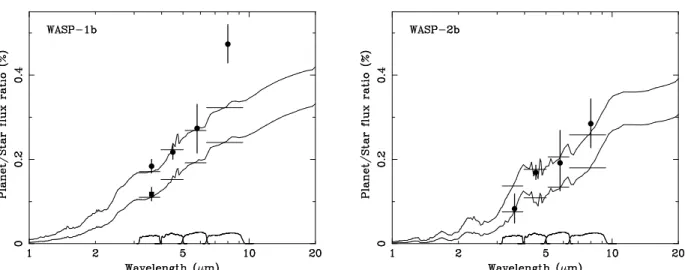
Our measured secondary-eclipse depths are compared with the planetary atmosphere models of Fortney et al. (2008) in Fig. 6. For WASP-1b the model predicts a stratospheric tem-perature inversion and the two curves represent calculations in which the planetary emission is either limited to the day side (upper curve) or is uniform over its entire surface (lower curve). For the 3.6µm band we include the eclipse depths
from both the linear decorrelation (circle) and the quadratic decorrelation (square). For WASP-2b, which is much less strongly irradiated, the model does not predict a temperature inversion and the two curves represent calculations for day-side emission (upper) and uniform emission (lower) as before. In order to aid comparison with measured eclipse depths we have calculated average planet/star flux ratios for each model in each IRAC band. These averages have been weighted using the IRAC spectral response curves (Hora et al. 2008), which are plotted at the bottom of each panel. The model averages in each band are represented by horizontal lines.
The 4.5µm and 5.8 µm eclipse depths of WASP-1b are
con-sistent with the model predicting a temperature inversion in this system and where emission is limited to the day side of the planet. The 5.8µm band is consistent also with uniform
emission, but the 4.5µm band is not. The 3.6 µm eclipse
depth with linear decorrelation is also consistent with the in-version model and day-side emission, but the same data fit-ted with quadratic decorrelation is not. Since the quadratic decorrelation provides a better fit to the data (Fig. 5), this sug-gests that the model is over-predicting the planetary flux in this band. Alternatively, it may be that the additional degrees of freedom in the quadratic decorrelation results in an under-estimate of the eclipse depth in this band.
The 8.0µm eclipse depth of WASP-1b lies significantly
above the model prediction (3.3σ). The inversion model
Figure 6. Secondary eclipse depths of the exoplanets WASP-1b and WASP-2b overlaid on the planetary atmosphere models of Fortney et al. (2008), which are plotted as fraction of the stellar flux. In both cases the upper curves represent models in which emission is only from the day-side of the planet, and the lower curves represent uniform emission from the entire exoplanet surface. For the 3.6 µm band of WASP-1b we have included eclipse depths from both linear decorrelation (circle) and quadratic decorrelation (square). The horizontal lines on each model represent averages in the IRAC bands weighted by the spectral responses of the camera, which are indicated with solid curves at the bottom of the plot.
model is under-predicting the strength of the temperature in-version in this system.
In WASP-2b, the eclipse depths in all four bands are con-sistent with the model predicting no temperature inversion and with emission only from the day side of the planet. The
3.6µm and 5.8 µm eclipses are consistent also with the
uni-form emission model, but the 8µm eclipse is only marginally
consistent with this model and the 4.5µm eclipse is
inconsis-tent (3.6σ).
As further illustration of the importance of the detected temperature inversion in WASP-1b, we have also compared the measured eclipse depths with a model calculation in which the temperature inversion has been artificially suppressed (by setting the TiO/VO abundances to zero in the model). The re-sults are plotted in Fig. 7 and show that the measured eclipse depths strongly favor the model with a temperature inversion. Table 3 includes updated system parameters for both plan-ets from our simultaneous analysis of the secondary-eclipse, primary-transit and radial-velocity data. Of particular interest is e cosω, which is constrained by the timing of the secondary
eclipses. A significant eccentricity is found from the lin-ear decorrelation fits to the WASP-1b light curves, however, this result is not supported by the quadratic decorrelation fits, where the deviation from zero drops to less than two-sigma. This fit places a tight three-sigma upper limit of|e cos ω| <
0.0033, suggesting that the inflated radius of WASP-1b is
un-likely to be due to tidal heating. We place a similar upper limit on the eccentricity of WASP-2b of|e cos ω| < 0.0040.
6. DISCUSSION
Overall our measured secondary eclipse depths of WASP-1b and WASP-2b in the four IRAC bands are in remark-ably good agreement with the predictions of the Fortney et al. (2008) model (Fig. 6; note that the model has not been fitted to the data). This model predicts an atmospheric temperature inversion in 1b (class pM) and no inversion in WASP-2b (class pL). In WASP-WASP-2b the agreement between the model and data is excellent in all four bands. In WASP-1b the depth of the 8µm eclipse indicates that the strength of the
tempera-ture inversion may be under-estimated in the model. In both planets the 4.5µm eclipse is the best defined and also the one
Figure 7. Secondary eclipse depths of the exoplanet WASP-1b overlaid on
planetary atmosphere models in which the temperature inversion has been artificially suppressed by setting the TiO/VO abundance to zero. As in Fig-ure 6, the upper curve represents a model with emission only from the day side of the planet, and the lower curve represents a model in which heat is transported efficiently around the planet. For the 3.6 µm band of WASP-1b we have included eclipse depths from both linear decorrelation (circle) and quadratic decorrelation (square). The horizontal lines show the weighted av-erages of the models in the four IRAC bands, with the IRAC band passes indicated by the solid curves at the bottom of the figure.
least affected by instrumental effects, and in both cases the eclipse depth in this band is consistent only with the day-side emission model. We take this as strong evidence that redistri-bution of incident energy is inefficient in both planets.
Our detection of a temperature inversion in WASP-1b but not in WASP-2b is consistent with expectations based on their different irradiation levels (2.5 × 10⁹erg s−1cm−2 and
0.9 × 10⁹erg s−1cm−2 respectively; Fortney et al. 2008). It
is also generally consistent with Spitzer measurements of other planets. Of the systems studied in all four IRAC bands, HD189733b, XO-2b and HAT-P-1b have irradiation levels at or below the expected transition of around 0.8 ×
109erg s−1cm−1, and do not show strong temperature
inver-sions, although XO-2b and HAT-P-1b do exhibit evidence for weak inversions (Charbonneau et al. 2008; Machalek et al.
2009; Todorov et al. 2010). HD209458b, 4 and TrES-2 have irradiation levels at or above the expected transition and all exhibit evidence for stronger temperature inversions (Knutson et al. 2008, 2009; O’Donovan et al. 2010). How-ever exceptions to this rule have also been found. XO-1b ex-hibits evidence for a temperature inversion despite irradiation at only 0.5 × 10⁹erg s−1cm−2 (Machalek et al. 2008, 2009),
while TrES-3 has not been found to do so, despite high ir-radiation at 1.6 × 10⁹erg s−1cm−2(Fressin et al. 2010).
To some extent the observational picture is confused by the different models applied by different authors, and the different criteria applied for the detection of a temperature inversion. Gillon et al. (2010) plotted a color-color diagram for planets studied in all four IRAC bands (their Fig. 10) and found that the planets studied to date cover a wide range of color space, and do not fall neatly into two distinct groups. In this paper we have presented a uniform analysis of secondary eclipse data from two planets for the first time. It may be that the obser-vational picture will become more clear once further uniform analyses of multiple systems are carried out.
In order to search for a pattern in published secondary eclipse depths, we have plotted the ratio of depths in the
8.0µm and 4.5 µm bands against irradiation in Fig. 8. We
chose to compare the ratio of these two bands since they (1) are available for the largest number of planets, (2) are sensi-tive to the strength of water emission/absorption at 8µm, (3)
are less affected by instrumental systematics than the 3.6µm
band. Our figure does not show a sharp transition at an ir-radiation level of around 0.8 × 10⁹erg s−1cm−2 as might be
expected from the predictions of Fortney et al. (2008), but it does show a gradual decrease of the flux ratio through this range. However, we do find tentative evidence for a sharp transition at a higher irradiation level of 2× 10⁹erg s−1cm−2.
The systems beyond this transition are TrES-4 (Knutson et al. 2009) and WASP-1b (this paper), both showing remarkably strong emission at 8µm, perhaps related to their high
irradia-tion levels.
This transition could be due to a change in the chemistry and opacity of the atmospheres at that level of incident flux. One possibility is that TiO gas is aloft at millibar pressures only at higher irradiation levels (and hotter atmospheres) and at lower irradiation (< 2 × 10⁹erg s−1cm−2) another absorber
is causing the observed inversions, such as a sulfur photo-chemical product (Zahnle et al. 2009). Both may operate over some range. It now appears likely that opacity due to gaseous TiO and VO is not the entire story. In particular, the atmo-sphere of XO-1b appears to be so cold that Ti should be se-questered into solid condensates at any location in the atmo-sphere. However, even at slightly warmer temperature in the upper atmosphere, there is the still the important issue of the temperature of the deep atmosphere.
Much attention has been paid to how cold traps may af-fect the abundance of TiO gas at millibar pressures. If Ti is trapped in solid condensates deep in the atmospheres at∼ 0.1
to 1 kbar, then it would require quite strong vertical mix-ing to enable gaseous TiO to exist in the upper atmosphere. This has been discussed by many authors (Hubeny et al. 2003; Fortney et al. 2006, 2008; Burrows et al. 2008) and calcu-lated in some detail by Showman et al. (2009) and especially Spiegel et al. (2009). For instance, there is good agreement that if TiO causes the temperature inversion for HD209458b, it must be mixed above the cold trap (Fortney et al. 2008; Spiegel et al. 2009). This is not a priori impossible. In
Nep-Figure 8. The ratio of secondary-eclipse depths at 8 µm and 4.5 µm for all
planets published to date (in planet/star contrast units), plotted as a function of irradiation by the parent star. The most highly irradiated planets, including WASP-1b, appear to be relatively brighter at 8 µm.
tune, abundant gaseous methane is found in the stratosphere, despite a cold trap that should condense methane in the tro-posphere (Fletcher et al. 2010, and references therein). How-ever, it is not yet clear whether this mixing through the cold trap happens in hot Jupiters.
Interestingly, Fortney et al. (2006) investigated the deep at-mosphere of HD149026b, which is at an irradiation level of 2× 10⁹erg s−1cm−2 and found that its atmospheric
tempera-tures sat on the cold trap dividing line (see their Fig. 2), which is a tantalizing suggestion that the break seen in Fig. 8 could be due to TiO. At higher irradiation levels there is no cold trap issue, although the exact location of this boundary is sen-sitive to the planet surface gravity and location of the radia-tive/convective boundary. We note that Spiegel et al., largely because they assumed colder interior temperatures, found that this division happened at higher irradiation levels. Additional data for the hottest objects will help to support or refute the trends shown in Fig. 8.
7. CONCLUSIONS
The measured secondary-eclipse depths of WASP-1b and WASP-2b presented here indicate a strong temperature sion in the atmosphere of WASP-1b, but no temperature inver-sion in WASP-2b. This difference is likely to be related to the much higher level of irradiation of the atmosphere of WASP-1b. The eclipse depths of both planets also favor models in which incident energy is not redistributed efficiently from the day side to the night side of the planet. We do not find sig-nificant eccentricity in the orbits of either planet, suggesting that the inflated radius of WASP-1b is unlikely to have arisen through tidal heating. Finally, we find evidence for a sharp transition in the properties of planetary atmospheres with irra-diation levels above 2× 10⁹erg s−1cm−2, and we suggest that
this transition might be due to the presence of TiO in the upper atmospheres of the most strongly irradiated hot Jupiters.
Facilities: Spitzer.
REFERENCES
Alonso, R., Guillot, T., Mazeh, T., Aigrain, S., Alapini, A., Barge, P., Hatzes, A., & Pont, F. 2009, A&A, 501, L23
Fazio, G. G., et al. 2004, ApJS, 154, 10
Fletcher, L. N., Drossart, P., Burgdorf, M., Orton, G., & Encrenaz, T. 2010, ArXiv e-prints
Ford, E. B. 2005, AJ, 129, 1706
Fortney, J. J., Lodders, K., Marley, M. S., & Freedman, R. S. 2008, ApJ, 678, 1419
Fortney, J. J., Marley, M. S., Lodders, K., Saumon, D., & Freedman, R. 2005, ApJ, 627, L69
Fortney, J. J., Saumon, D., Marley, M. S., Lodders, K., & Freedman, R. S. 2006, ApJ, 642, 495
Fressin, F., Knutson, H. A., Charbonneau, D., O’Donovan, F. T., Burrows, A., Deming, D., Mandushev, G., & Spiegel, D. 2010, ApJ, 711, 374 Gillon, M., et al. 2010, A&A, 511, A3+
Grillmair, C. J., Charbonneau, D., Burrows, A., Armus, L., Stauffer, J., Meadows, V., Van Cleve, J., & Levine, D. 2007, ApJ, 658, L115 Harrington, J., Luszcz, S., Seager, S., Deming, D., & Richardson, L. J. 2007,
Nature, 447, 691
Hora, J. L., et al. 2008, PASP, 120, 1233
Hubeny, I., Burrows, A., & Sudarsky, D. 2003, ApJ, 594, 1011 Knutson, H. A., Charbonneau, D., Allen, L. E., Burrows, A., & Megeath,
S. T. 2008, ApJ, 673, 526
Knutson, H. A., Charbonneau, D., Burrows, A., O’Donovan, F. T., & Mandushev, G. 2009, ApJ, 691, 866
2007, Nature, 445, 892
Seager, S., Richardson, L. J., Hansen, B. M. S., Menou, K., Cho, J. Y.-K., & Deming, D. 2005, ApJ, 632, 1122
Showman, A. P., Fortney, J. J., Lian, Y., Marley, M. S., Freedman, R. S., Knutson, H. A., & Charbonneau, D. 2009, ApJ, 699, 564
Shporer, A., Tamuz, O., Zucker, S., & Mazeh, T. 2007, MNRAS, 376, 1296 Sing, D. K., & López-Morales, M. 2009, A&A, 493, L31
Sing, D. K., Vidal-Madjar, A., Lecavelier des Etangs, A., Désert, J., Ballester, G., & Ehrenreich, D. 2008, ApJ, 686, 667
Snellen, I. A. G., de Mooij, E. J. W., & Albrecht, S. 2009, Nature, 459, 543 Spiegel, D. S., Silverio, K., & Burrows, A. 2009, ApJ, 699, 1487 Swain, M. R., Vasisht, G., Tinetti, G., Bouwman, J., Chen, P., Yung, Y.,
Deming, D., & Deroo, P. 2009a, ApJ, 690, L114 Swain, M. R., et al. 2009b, ApJ, 704, 1616
Todorov, K., Deming, D., Harrington, J., Stevenson, K. B., Bowman, W. C., Nymeyer, S., Fortney, J. J., & Bakos, G. A. 2010, ApJ, 708, 498 Werner, M. W., et al. 2004, ApJS, 154, 1
Zahnle, K., Marley, M. S., Freedman, R. S., Lodders, K., & Fortney, J. J. 2009, ApJ, 701, L20