HAL Id: hal-03241432
https://hal.archives-ouvertes.fr/hal-03241432
Submitted on 31 May 2021
HAL is a multi-disciplinary open access archive for the deposit and dissemination of sci-entific research documents, whether they are pub-lished or not. The documents may come from teaching and research institutions in France or abroad, or from public or private research centers.
L’archive ouverte pluridisciplinaire HAL, est destinée au dépôt et à la diffusion de documents scientifiques de niveau recherche, publiés ou non, émanant des établissements d’enseignement et de recherche français ou étrangers, des laboratoires publics ou privés.
Quantitative Analysis of Solidification of Compacted
Graphite Irons – A Modelling Approach
Jacques Lacaze, Anna Regordosa, Jon Sertucha, Urko de La Torre
To cite this version:
Jacques Lacaze, Anna Regordosa, Jon Sertucha, Urko de La Torre. Quantitative Analysis of Solidifica-tion of Compacted Graphite Irons – A Modelling Approach. ISIJ internaSolidifica-tional, Iron & Steel Institute of Japan, 2021, 61 (5), pp.1539-1549. �10.2355/isijinternational.ISIJINT-2020-476�. �hal-03241432�
1
Quantitative analysis of solidification of compacted graphite irons – A modelling approach.
J. Lacaze
a, A. Regordosa
b, J. Sertucha
b, U. de la Torre
ba - CIRIMAT, ENSIACET, Université de Toulouse, Toulouse, France
b - Investigación y Desarrollo de Procesos Metalúrgicos, Fundación Azterlan,
Durango (Bizkaia), Spain
abstract
Several X-ray topography studies which have appeared recently in the literature show compacted graphite in cast iron consisting of coarse interconnected graphite lamellas. This suggested that solidification of these alloys could be described as done for irregular eutectics by accounting for limited branching of graphite lamellas. The corresponding growth law has been inserted in appropriate mass balances for describing the successive solidification stages. Predictions of the model thus obtained have been compared to quantitative experimental information previously gained on solidification of a series of hyper-eutectic alloys. The deep undercooling and marked recalescence which are so characteristic of the solidification of compacted graphite cast irons in the stable system are reproduced and appear to be closely related to the limited branching of graphite lamellas in the compacted graphite cells. The competition between stable and metastable
solidification could be described and leads to a decrease of the recalescence amplitude that was properly reproduced.
2 Introduction
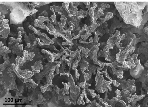
Thanks to detailed metallographic studies [1,2] and to recent tomography results [3,4], it is now well established that graphite in compacted graphite (CG) cells consists of interconnected thick lamellas with bumpy surfaces as illustrated in figure 1. Because of the appearance of CG as worm-like particles in 2D sections with sometimes hemispherical caps, many early studies [5,6] concluded that the overall growth direction should be the basal plane direction as in spheroidal graphite. This however appears contradictory with the lamellar growth shape shown with recent tomographic results. A detailed study combining observations with polarized light microscopy and scanning electron microscopy (SEM) of deep etched and ion etched samples led Franklin to the conclusion that the main growth direction of compacted graphite is parallel to the basal plane of graphite [7], i.e. along the prismatic direction. This was further confirmed more recently by Holmgren et al. [8] who observed by electron backscattering diffractometry (EBSD) that worm-like graphite particles are oriented along the prismatic direction as lamellar graphite while protuberances seem to develop in the basal direction as in spheroidal graphite. Accepting that growth of CG cells proceeds mainly as those in lamellar graphite irons, it has been proposed that the main difference between lamellar and compacted graphite structure is the very limited branching of the lamellas in compacted graphite iron (CGI) [9,10].
Figure 1 – SEM view a CG cell after deep etching of the material to remove the matrix (courtesy of W. Guesser).
3 It seems also agreed that the CG cells develop around previously precipitated graphite spheroids [11,12] as a kind of graphite degeneracy [6]. In the case of hypereutectic alloys, the observation of large primary graphite spheroids sustains this claim. The same schematic has been accepted by Lopez et al. [13] for hypoeutectic alloys. It is not unusual to observe also small nodules in CGI which formed at the end of solidification; they have been associated to a combination of large undercooling and Mg micro-segregation during bulk eutectic solidification [14,15].
Based on the above view of CGI solidification, a physical model of solidification of CGI is described for the case of hypereutectic composition. This model is then applied to experimental results on non-inoculated alloys which have been detailed previously [16,17] and relate to solidification in small thermal analysis cups.
Physical modelling
Figure 2 shows the isopleth Fe-C section at 3.65 wt.% C, 0.83 wt.% Cu, 0.62 wt.% Mn and 2.39 wt.% Si, that is representative of the final composition of the experimental alloys. The data used to draw this section have been detailed previously [17] and are summarized in annex A. This isopleth section shows the stable diagram in solid lines with their metastable extrapolation drawn with interrupted lines. The austenite solidus was calculated assuming a constant carbon partition coefficient
47
.
0
k
C/l
between austenite, , and liquid, l. The horizontal dashed lines show the stable, TEUT, andmetastable, TEW, eutectic temperatures which were calculated as indicated in annex A.
In all the following, the alloys will be considered as pseudo binary Fe-C alloys and their solidification will be described in the isopleth section such as that shown in figure 2. On this figure, the
solidification path of a hypereutectic alloy is represented with thin solid lines along 3 successive steps labelled a, b and c, that are described as follows. When the temperature is decreased from the full liquid state, the solidification path reaches the graphite liquidus at G
L
T where graphite starts precipitating. Nucleation and growth of these precipitates is described as for spheroidal graphite [18], see annex B. Because growth of graphite is partly controlled by an interfacial reaction, the solidification path is located below the graphite liquidus as shown with label a in figure 2, which corresponds to the schematic microstructure in figure 3-a.
When the metastable extrapolation of the austenite liquidus is reached at TLA, formation of austenite
dendrites and CG cells may proceed, see figure 3-b. It is assumed that equilibrium at the
liquid/austenite interface is achieved at any time, meaning that there is no nucleation barrier for austenite and that the composition of the remaining liquid follows the austenite liquidus as indicated
4 with the label b in figure 2. The experimental results [17] suggest that there is little or no further nucleation of graphite during this stage, so that the number of CG cells could be fixed as the nodule count reached at the end of primary deposition. The equations describing the eutectic reaction in annex C have been derived for single sized primary graphite, i.e. an equivalent radius RGE has been
calculated. This is not expected to affect much the calculations as compared to those which could have been made with a size distribution of the primary graphite precipitates, and this makes the equations much lighter.
Figure 2 – In bold lines is shown the isopleth Fe-C section of the Fe-C-Si-Mn-Cu phase diagram at 0.83 wt% Cu, 0.62 wt.% Mn and 2.39 wt.% Si; the interrupted parts of the lines are metastable
extrapolations. The thin horizontal dashed lines indicate the temperature of the stable, TEUT, and
metastable, TEW, eutectics in this isopleth section. Thin solid lines represent schematically the
solidification path of a hypereutectic alloy and the thin horizontal doted lines show the corresponding characteristic temperatures, TLG and TLA.
Finally, if the temperature falls below the temperature of the metastable eutectic, TEW, nucleation of
ledeburite is assumed instantaneous. During further solidification, growth of CG cells and ledeburite proceeds (see figure 3-c) while the solidification path still follows the austenite liquidus as indicated with label c in Figure 2.
1050 1100 1150 1200 1250 1300 1.0 1.5 2.0 2.5 3.0 3.5 4.0 4.5 5.0 Tempera tu re (° C) Carbon content (wt.%) graphite liquidus austenite liquidus austenite solidus T EW T EUT a b c T LA G L T
5 Figure 3 – Schematic illustrating the three successive steps in the solidification of an hypereutectic CGI as labelled in figure 2: a) precipitation of primary graphite; b) growth of off-eutectic austenite dendrites and of CG cells; c) additional formation of ledeburite cells.
While annexes B and C detail the overall kinetics equations, it is worth considering in this section the way growth of the CG cells is to be quantitatively described. According to the introductory part, growth of CG cells is similar to that of irregular eutectics, e.g. lamellar graphite eutectic. The peculiarities of these eutectics have been described in the early 1980s by Fisher and Kurz [19] and more particularly by Jones and Kurz [20] for the case of the austenite-graphite system. The authors based their analysis on the classical work by Jackson and Hunt [21] who stated the following relationship between eutectic undercooling, T, lamellar spacing, , and growth rate, Vgrowth:
T a b Vgrowth (1)
In figure 4, the solid curves represent relation (1) for three growth rates Vgrowth (0.1, 1 and 10 µ·ms-1)
using the values of a and b estimated by Jones and Kurz [20]: a=2.3 µm·K and b=0.080 K·s·µm-2. By stating that growth proceeds at the minimum undercooling one gets the following relationships:
a
graphite liquidb
austenite dendrite CG cellsc
ledeburite6 growth 0
V
b
a
(2) growth 02
a
b
V
T
(3) 0 0 a 2 T (4)where the subscript 0 refers to the so-called extremum condition for velocity Vgrowth.
Figure 4 – The solid lines show the theoretical evolution of the eutectic undercooling with interlamellar spacing for solidification rates indicated on the curves. The dashed lines show the position of the operative point for two values of , namely 1 which corresponds to the minimum undercooling and 10 which corresponds to the branching limit.
Experimental results on growth of lamellar graphite eutectic show that the spacing is distributed over quite a large range [20]. The boundaries of this range were set to 0 for the smallest value and
br for the largest one. br is the value at which branching of graphite lamellas must occur for
two-phase growth to be maintained. Because of the faceted nature of graphite, branching is quite difficult, and this is thought to explain why br has been found to be as large as about 10 times 0 in
lamellar graphite eutectic [20]. Assuming the diffusional analysis of Jackson and Hunt remains valid, Jones and Kurz suggested defining an operating interlamellar spacing, op, such as:
0.1 1 10 100 1000 0 1 10 100 1000 Eut ect ic und e rc ool ing (° C) Interlamellar spacing (µm) 0.1 µm/s 1.0 µm/s 10 µm/s
7 growth 0 op
V
b
a
(5)By substitution of op in equation (1), one gets the following expressions for the operating
undercooling Top:
growth 2 op 1 a b V 1 T (6)
op 2 opa
1
T
(7)This latter relation has been plotted with interrupted lines in figure 4 for =1 which corresponds to the extremum and =10 that relates to the branching limit of graphite lamellas. Following this line, the growth rate of spherical compacted graphite cells of radius RCG will be related to the eutectic
undercooling by the following relation where a and b are the values assessed by Jones and Kurz [20]:
b a 1 T dt dR 2 2 CG (8) where RCG is in µm.Jones and Kurz [20] could fit their results of directional solidification experiments with set to 3.9 while Zou Jie [22] found a value of 6.5 for equiaxed solidification of an Fe-C-Si alloy. Zou Jie suggested that part of the difference with directional solidification results is due to the expanding nature of the eutectic cells in equiaxed solidification. As stressed above in the case of CG cells, the protuberances that form on the primary graphite precipitates then develop without much branching. Thus, the distance between them increases as the size of the CG cells increases and should thus reach quickly a high value. This suggested setting to a maximum value which should be of the order of 10 where branching of graphite lamellas is expected.
Finally, growth of ledeburite is to be described as spherical cells of radius RW using the data from
Hillert and Subba Rao [23] which is very close to the value later found by Jones and Kurz [20]:
2 W30
T
dt
dR
(9) where RW is in µm.8 With equations (8) and (9), the change in volume of solid
dt dVS
at any time step t during the
eutectic reaction can be calculated as described in annex C. This volume change is then to be inserted in the heat balance equation representing homogenous cooling of a volume V of metal having an outer surface A (V/A is the casting modulus) [24,25]:
0
0.5 S p T T t dt V / dV H dt dT C A / V (10)where and Cp are, respectively, the density and the heat capacity of the metal at temperature T, H
is the latent heat of fusion of the metal, is a quantity characteristic of the mold and T0 is the ambient temperature. The data used in the present calculations are listed in table 1, they are the same as those previously selected [18, 24] except for
as described in the next section. During solidification, the specific heat Cp and the density were calculated as a weighted average of thesolid and liquid values.
Following previous works, the exponent n of the nucleation law for primary precipitation of graphite (see annex B) was set to 1 so that the nucleation constant is denoted as A1 in the following. Also, it
was assumed that a given number of ledeburite cells nucleated as soon as the TEW temperature was
reached. The outputs of the calculations are marginally sensitive to the exact value of this number which was set to 0.5 mm-3.
Table 1 – Values of the parameters that were used for calculations. V/A [m] [J·m
-2 ·K-1·s-0.5] p C [J·K-1·kg-1] [kg·m-3] K [m·s-1] H [J·kg-1] 0.009 728 before solidification 1215 after solidification Liquid: 920 Solid: 750 Liquid: 6800 Austenite: 7000 Graphite: 2200 0.05 Graphite: 1.62·106 Iron: 2.56·105In the following sections, all microstructure parameters keep the same name as in annexes B-D but they are now for a unit volume. This means that NV is a count density and that VS, VCG and V,off are
volume fractions.
Preliminary calculations
The experiments considered here have been fully described previously [17] and are only shortly presented below. A 4 ton melt prepared for casting spheroidal graphite cast iron was maintained for
9 8 hours under helium so that the spheroidizing treatment faded slowly leading to precipitation of compacted graphite. Every 20-25 min, two thermal analysis (TA) cups and a medal for chemical analysis were cast; 19 castings were thus carried out which were labelled A to S. One cup was empty while the other contained an inoculant powder, so that the two samples cast at a given holding time were denoted Xinoc and Xno-inoc, respectively, where X is a letter from A to S. Chemical analysis showed
the alloys lose only up to about 0.1 wt.% carbon and 0.06 wt.% silicon during the 8 h holding, but also a much higher proportion of spheroidizing elements Mg, Ce and La. The cooling curves of the
inoculated alloys consisted in one single plateau which did not show much change with holding time although the microstructure changed from fully spheroidal to nearly fully compacted. In strong contrast, the cooling curves for the not-inoculated alloys showed a minimum temperature that decreased continuously with holding time, being below TEW after less than 1 hour. The graphite
changed from spheroidal to compacted while more and more carbides were observed. Non-inoculated castings did thus contain much more information than the Non-inoculated ones and were accordingly selected for the present work as they are more challenging for checking the validity of the modelling approach.
For performing the calculations for the whole series of alloys, it was intended to have as few parameters as possible. Preliminary calculations dedicated to fit the cooling rates before and after solidification led to select a modulus of 0.009 m and a value of
differing for cooling of the liquid and of the solid, see table 1. During the solidification stage,
was calculated as a weighted average of the solid and liquid values. The only quantity related to heat transfer that could then be changed from one calculation to another is the initial temperature of the melt which can be slightly larger than the maximum temperature, Tpeak, recorded by the thermocouple of the TA cup. It wasfound convenient to set this initial temperature at Tpeak+30°C for all calculations. Calculations
accounted for the slight changes in alloy composition and Tpeak from one alloy to the other, so that
the only parameter left for describing solidification was the nucleation constant A1.
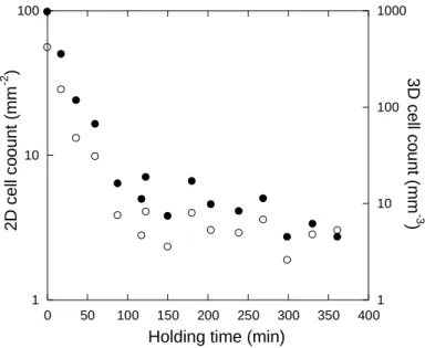
Focus was then first put on the number of graphite spheroids nucleated during primary precipitation of graphite. According to the assumptions indicated above, this number equals the CG cells count that will develop during the eutectic reaction. Figure 5 shows the evolution of the experimental cell count as evaluated on 2D sections, NA, and then converted to 3D values, NV, by
2 A V D N 2 N [26],
where D2 is the average diameter of the CG cells measured on the 2D section. NA and D2 values
10 calculation to another in order to agree with the evolution seen in figure 5, with the only constraint that it should decrease with the holding time of the melt.
Figure 5 – Evolution of the 2D (solid symbols) and 3D (open symbols) experimental cell counts with holding time of the melt.
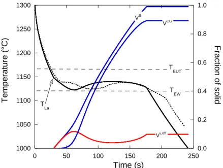
As an example, figure 6 compares the evolution of the calculated and experimental temperatures for alloy Cno-inoc with A1=0.5 mm-3·K-1. It is seen an overall good agreement between the calculated and
experimental cooling curves with however a time shift of the experimental curve at the start of eutectic solidification which is not reproduced by the calculation and will be discussed further below. Also shown in figure 6 are the predicted overall solid fraction, VS, the amount of off-eutectic
austenite, V,off, and that of CG eutectic, VCG. Primary precipitation of graphite is not plotted because the fraction was always very low at less than 1%. It is seen that this is mainly austenite that deposits at the start of solidification. The amount of CG eutectic remains very low until the temperature falls down to just above 1120°C when bulk eutectic sets up with recalescence due to rapid growth of eutectic cells, while part of the off-eutectic austenite remelts before growing again. It is noteworthy that the value of =10 that was selected leads to a fairly good description of the recalescence amplitude.
In the calculations as the one shown in figure 6, formation of austenite at the end of primary precipitation of graphite leads to a slope change at the TLA temperature that is indicated with the
open arrow in the figure. In contrast, all experimental cooling curves for not inoculated alloys B-S showed a slope change soon followed by a short plateau similar to that seen in Figure 6. Further, calculation for the whole series of alloys made it evident that the experimental TLA value was lower
1 10 100 1 10 100 1000 0 50 100 150 200 250 300 350 400 2D cell co ou nt ( mm -2 ) 3D cel l co un t (mm -3 )
11 than the calculated one. This is illustrated in figure 7 where it is seen that the experimental values vary in between 1138 and 1153°C and that they are 5 to 10°C lower than the calculated values. The change in the experimental value of TLA was observed to be an overall increase with holding time
[17]. As a matter of fact, the TLA value is expected to increase when: i) the pouring temperature is
increased leading to lower cooling rate; ii) the carbon equivalent of the alloy is decreased; and iii) the graphite nucleation rate is increased. In fact, most of the change in the experimental TLA value could
be accounted for by the decrease in carbon content of the alloys with holding time as discussed previously [17]. Change in the pouring temperature could account for a smaller part of the variation, and dedicated calculations (not shown here) demonstrated that the effect of graphite nucleation is negligible for the range of A1 values used here. Summing up, the good linear correlation seen in
figure 7 demonstrates that the model for primary precipitation of graphite accounts properly of the change in composition and pouring temperature of the alloys, though not describing the systematic undercooling for austenite formation which amounts to 5-10°C. It is noteworthy that this
undercooling is well within the range of values discussed by Heine [27].
Figure 6 – Experimental (dotted curve) and calculated (solid curve) cooling curves for alloy Cno-inoc.
Also shown are the predicted overall solid fraction, VS, the amount of off-eutectic austenite, V,off, and that of CG eutectic, VCG. The open arrow indicates the TLA value which corresponds to the
temperature when the calculated primary solidification path reaches the extrapolation of the austenite liquidus. 1000 1050 1100 1150 1200 1250 1300 0.0 0.2 0.4 0.6 0.8 1.0 0 50 100 150 200 250 T e mpe rature (° C ) Fr actio n of soli d Time (s) VCG VS V,off T EW T EUT T La
12 Figure 7 – Experimental versus calculated TLA values. The solid line is linear fit to the data while the
interrupted line is the bisector.
Owing to the small size of the thermal cup, it is expected that austenite develops from the outer surface of the cup towards the center as described by Mampaey by means of quenching experiments of rods of similar size as the TA cups [28, 29]. For such a columnar growth, the thermal arrest when the solidification front reaches the thermocouple is not expected to give rise to recalescence, and recalescence was effectively not observed in the present series of records. In turn, this means that the 5-10°C temperature difference is due to the kinetic undercooling of the front of austenite dendrites. The growth rate Vgrowth of austenite cells and dendrites has been previously theoretically calculated as a function of tip undercooling Ttip for Fe-C-Si alloys [30]. In the dendritic regime, a
relation between Vgrowth (µm/s) and Ttip (°C) can be expressed as: Vgrowth 1.01
Ttip
2.60. For anundercooling of 10°C, the time needed for the austenite dendrite front to travel the 17.25 mm from the surface of the thermal cup to the thermocouple junction is thus calculated to be 43 s. This time is quite similar to the time shift observed in the experimental records.
It is expected that a 3D micro-macro modelling of the solidification of the thermal cups would allow recovering the feature described above. For the present approach, it was decided to amend the model by introducing an undercooling of the liquid Ttip before austenite appears in the central area
of the TA cups. The solidification path was then changed as illustrated with figure 8 with austenite starting to form only when the temperature (TLA-Ttip) has been reached. At that temperature, CG
cells start growing and a linear increase with time of the austenite fraction at constant temperature
1135 1140 1145 1150 1155 1160 1165 1135 1140 1145 1150 1155 1160 1165 C a lcu la ted T LA v a lu e (° C ) Experimental T LA value (°C)
13 is assumed as described in annex D. The path followed is schematically shown with the segment A-B in figure 8, it corresponds to what can be called a pre-eutectic reaction [31]. When the carbon content in the liquid reaches that of the austenite liquidus extrapolation, this “transitory” step ends and solidification then proceeds along b and then c. In the calculations shown in the next section,
Ttip was set to 10°C.
Figure 8 – Same as figure 2 but with primary deposition of graphite ending when the temperature equals (TLA-Ttip). The solidification path then follows the line segment A-B to reach the metastable
extrapolation of the austenite liquidus, and finally continues along b and c.
Results
The values of A1 were evaluated assuming a continuous decrease of the nucleation constant from
alloy Ano-inoc to alloy Sno-inoc. Its value was thus first estimated to fit the cell count for alloys Ano-inoc and
Sno-inoc, and for a couple of intermediate alloys, and then a smooth variation was set up. Note that the
composition and the pouring temperature of each alloy listed previously [17] were considered in the calculations. The values used for A1 are plotted in figure 9 where are also compared the calculated
and experimental CG cell counts. The figure shows a marked decrease of the number of cells from alloy A to alloy E, i.e. the first 80 minutes of holding, and then a smoother decrease. Although the
1050 1100 1150 1200 1250 1300 1.0 1.5 2.0 2.5 3.0 3.5 4.0 4.5 5.0 Tempera tu re (° C) Carbon content (wt.%) graphite liquidus austenite liquidus austenite solidus T EW T EUT a b c A B G L T LA T Ttip
14 related decrease of A1 was monotonous (see the crosses in figure 9), some slight scattering in the cell
count is observed which has to do with the variations in alloy composition and pouring temperature.
Figure 9 – Experimental and calculated CG cell counts (mm-3) and values of A1 (mm-3·K-1) used for the
calculations.
In Figure 10 is plotted the evolution with time of the calculated and experimental cooling curves for alloy Cno-inoc after the modification of the model discussed in relation with figure 6. It is seen that the
calculated curve shows now a pre-eutectic plateau which mimics satisfactorily the experimental one. The predicted evolution of the overall solid fraction, VS, the amount of off-eutectic austenite, V,off, and that of CG eutectic, VCG, are also shown. As before, the amount of off-eutectic austenite first increases, then slightly decreases during recalescence and finally increases again. This decrease is related to melting back of some off-eutectic austenite which is necessary for the composition of the remaining liquid to follow the austenite liquidus (stage b) as assumed. It is seen in figure 10 that the experimental minimum temperature and amplitude of recalescence are perfectly reproduced by calculations. In order to better reproduce the very end of solidification, the correction factor which allows accounting for impingement of the growing eutectic cells (see annex C) was changed from the Avrami’s factor used for figure 6 to 1.5 for this and all other calculations.
0 0.1 1 10 100 1000 A B C D E F G H I J K L M N O P Q R S experimental 3D cell count calculated cell count A 1 Ce ll n umb er (mm -3 ) an d A 1 value Alloy reference
15 Figure 10 – Experimental (dotted curve) and calculated (solid curve) cooling curves for alloy Cno-inoc.
Also shown are the predicted overall solid fraction, VS, the amount of off-eutectic austenite, V,off, and that of CG eutectic, VCG.
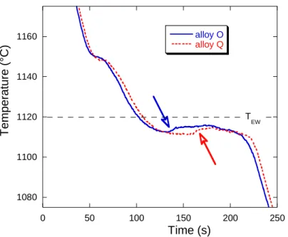
Contrary to the case of the first four alloys A-D, all cooling curves for alloys from E to S had a minimum temperature before recalescence below TEW [17], meaning ledeburite could form early
during bulk eutectic growth. All the experimental cooling curves were thus scrutinized and it was found that most of them showed a sharp temperature increase of about 3-4°C such as those
illustrated with open arrows in figure 11. These sharp arrests are much alike that reported by Lueben [32]. This feature should be associated to the formation of ledeburite as the growth rate of newly nucleated CG cells could not be high enough for generating such a nearly instantaneous
recalescence. What was more surprising is that this thermal arrest could be located anywhere in the first half of the eutectic plateau. This suggested that this arrest relates to the front of a ledeburite cell passing close to the thermocouple junction. In turn, this means that the experimental minimum temperature may show some scattering depending on the actual solidification microstructure developing nearby the thermocouple junction.
The above description suggests also that the temperature indicated by the thermocouple could be an average of the temperature at different growth fronts within a few cubic millimeters around the junction. This could explain that the temperature of the eutectic plateau in figure 11 is significantly below TEW while growth of ledeburite is expected to proceed at very low undercooling. It was thus
concluded that ledeburite did effectively appear in the center of all samples E to S as soon as the temperature felt below TEW, i.e. that there was a negligible nucleation barrier for it.
1000 1050 1100 1150 1200 1250 1300 0.0 0.2 0.4 0.6 0.8 1.0 0 50 100 150 200 250 T emp e ra tur e (° C ) Fra cti o n of so lid Time (s) VCG VS V,off T EW T EUT
16 Figure 11 – Experimental cooling curves of alloys O and Q showing a sharp thermal arrest (open arrows) during the eutectic plateau.
Figure 12 shows the resulting competition between stable and metastable eutectics in the case of alloy F. After the pre-eutectic plateau, the temperature decreases and the CG cells start growing as seen with the calculated VCG curve. However, the overall solidification rate is yet too low at this stage to avoid the temperature to fall below TEW. Slightly below this temperature, ledeburite is thus
predicted to start growing which gives a very small recalescence of about 1°C. For a while, the temperature remains just below TEW while both CG cells and ledeburite are growing. Later, the CG
cells have become large enough and the associated heat release makes the temperature overtake TEW. Accordingly, growth of ledeburite then stops and its fraction remains constant during a large
part of the eutectic plateau, see the VW curve. At the end of solidification, as the temperature falls again, ledeburite appears again and gives a marked horizontal arrest on the calculated curve which is not seen on the experimental one. This is thought to be due to microsegregation building up as silicon is rejected ahead of the growth front of ledeburite and thus lowering its growth rate, a feature that is not considered in the present modelling approach.
The fraction of cementite has been measured and it was noticed that the image analysis procedure could not differentiate cementite and ferrite in rod-like ledeburite [17]. This means that when the metastable eutectic appeared as clearly separated cementite plates, the values measured were the fractions of cementite, but that when cementite appeared as rod-like ledeburite this was the amount of metastable eutectic that was measured. The comparison which is made of experimental and
1080 1100 1120 1140 1160 0 50 100 150 200 250 alloy O alloy Q Temp erat ure (° C) Time (s) T EW
17 predicted values in figure 13 shows large scattering and discrepancies that are thought to be due to this difficulty in image analysis. However, it is noted that the expected trend of increasing fraction of metastable eutectic with holding time, i.e. with the decrease of the CG cell count, is effectively observed.
Figure 12 – Experimental (dotted curve) and calculated (solid curve) cooling curves for alloy Fno-inoc.
Also shown are the predicted overall solid fraction, VS, the amount of off-eutectic austenite, V,off, of CG eutectic, VCG, and that of ledeburite, VW.
Figure 13 – Comparison of the measured amount of carbide and the predicted amount of white eutectic for the whole series of alloys.
1000 1050 1100 1150 1200 1250 1300 0.0 0.2 0.4 0.6 0.8 1.0 0 50 100 150 200 250 Temp er a tur e (° C) Fractio n o f solid Time (s) VCG VS V,off VW TEW T EUT 0 0.1 0.2 0.3 0.4 0.5 A B C D E F G H I J K L M N O P Q R S experimental calculated F ract io n of le d e buri te Alloy reference
18 Finally, it is worth checking if the recalecence process which is so typical of CGI is properly
reproduced by the calculations. For solidification proceeding in the stable system, figure 10 shows a large recalescence. When there is a competition between stable and metastable eutectics as in figure 12, most of the recalescence may be associated to growth of the CG cells if the temperature
overtakes TEW during the eutectic plateau. However, as the holding time of the melt increases, the
number of CG cells decreases and eutectic recalescence fades until the eutectic plateau is nearly flat except for some vertical shift such as illustrated in figure 11. Figure 14 presents a comparison of experimental and calculated recalescence values for the whole series of alloys. It is seen that as the number of CG cells starts decreasing, recalescence strongly increases – from alloy Ano-inoc to alloy D no-inoc – and then decreases when ledeburite precipitates concurrently during bulk eutectic solidification
in agreement with previous work [11]. The experimental trend is quite well reproduced by the calculations and this comparison lands support to the description of the growth of CG cells that has been adopted in this work.
Figure 14 – Comparison of calculated and experimental recalescence values for the whole series of alloys.
Conclusion
The main features of the solidification of not inoculated hypereutectic compacted graphite irons as recorded by thermal analysis could be reproduced with quite a simple approach. Deep undercooling and marked recalescence which are so characteristic of CGI solidification in the stable system appear
0 5 10 15 20 A B C D E F G H I J K L M N O P Q R S experimental calculated Recal escence (°C) Alloy reference
19 to be closely related to the proposal that branching of graphite lamellas occurs at the extreme limit of coupled growth. The competition between stable and metastable solidification could be described and leads to a decrease of the recalescence rate as compared to a solidification proceeding entirely in the stable system. Owing to the fact that inoculation must be limited when casting CGI, the present work suggests to slightly increase the amount of silicon in these alloys in order to further decrease the metastable eutectic temperature, i.e. to slightly open up the window for stable solidification.
References
[1] C.R. Loper, R.C. Voigt, J.R. Yang, G.X. Sun, Use of the scanning electron microscope in studying growth mechanisms in cast irons, AFS Trans., 89, 1981, 529.
[2] Den Xijun, Zhu Peiyue, Liu Qifu, Structure and formation of vermicular graphite, Mat. Res. Soc. Symp. Proc., 34, 1985, 141-150.
[3] C. Chuang, D. Singh, P. Kenesei, J. Almer, J. Hryn, R. Huff, 3D quantitative analysis of graphite morphology in high strength cast iron by high-energy X-ray tomography, Scripta Mater., 106, 2015, 5-8; and https://www.anl.gov/article/highenergy-xrays-give-industry-affordable-way-to-optimize-cast-iron.
[4] K. Salomonsson, A.E.W. Jarfors, Three-Dimensional Microstructural Characterization of Cast Iron Alloys for Numerical Analyses, Proc. SPCI-XI, edited by A. Diószegi, V.L. Diaconu and A.E.W. Jarfors, Trans. Tech. Pub., Zurich, 925, 2018, 427-435.
[5] P.C. Liu, C.R. Loper, Scanning electron microscope study of the graphite morphology in cast iron, Scanning Electron Microscopy, 1, 1980, 407-418.
[6] Chen J.Y., Wu D.H., Liu P.C., Loper C.R., Liquid metal channel formation in compacted/vermicular graphite cast iron solidification, AFS Trans. 94, 1986, 537-544.
[7] S.E. Franklin, A study of graphite morphology control in cast iron, Loughborough University of Technology, 1986.
[8] D. Holmgren, R. Källbom, I.L. Svensson, Influences of the graphite growth direction on the thermal conductivity of cast iron, Metall. Mater. Trans. A, 38, 2007, 268-275.
[9] J. Lacaze, J. Sertucha, Some paradoxical observations about spheroidal graphite degeneracy, China Foundry, 15, 2018, 457-463.
[10] J. Lacaze, D. Connétable, M.J. Castro de Roman,Effects of impurities on graphite shape during solidification of spheroidal graphite cast ions, Materialia, 8, 2019, 100471, DOI:
10.1016/j.mtla.2019.100471
[11] Stefanescu D., Loper C.R., Voigt R.C., Chen I.H., Cooling curve structure analysis of
compacted/vermicular graphite cast irons produced by different melt treatments, AFS Trans. 1982, 333-348.
[12] J.M. Guilemany, N. Llorca, Metallographic differences between compacted graphite cast iron and vermicular graphite cast iron, Pract. Met., 21, 1984, 299-306.
[13] M.G. Lopez, G.L. Rivera, J.M. Massone, R.E. Boeri, Study of the solidification structure of compacted graphite cast iron, Int. J. Cast Met. Res., 29, 2016, 266-271.
20 [15] M. König, Microstructure formation during solidification and solid-state transformation in compacted graphite iron, PhD thesis, Chalmers University of Technology, 2011.
[16] A. Regordosa, U. de la Torre, A. Loizaga, J. Sertucha, J. Lacaze, Microstructure changes during solidification of cast irons - Effect of chemical composition and inoculation on competitive spheroidal and compacted graphite growth, Int. J. Metalcasting, 14, 2020, 681-688. DOI : 10.1007/s40962-019-00389-y
[17] A. Regordosa, U. de la Torre, J. Sertucha, J. Lacaze, 2020, Quantitative analysis of the effect of inoculation and magnesium content on compacted graphite irons – Experimental approach, Journal of Materials Processing Technology, in press
[18] G. Lesoult, M. Castro, J. Lacaze, Solidification of spheroidal graphite cast irons – I. Physical modelling, Acta Mater., 46, 1998, 983-995.
[19] D.J. Fisher, W. Kurz, A theory of branching limited growth of irregular eutectics, Acta Metall., 28, 1980, 777-794.
[20] H. Jones, W. Kurz, Relation of interphase spacing and growth temperature to growth velocity in Fe-C and Fe-Fe3C eutectic alloys, Z. Metallknde, 72, 1981, 792-797.
[21] K.A. Jackson, J.D. Hunt, Lamellar and rod eutectic growth, Trans. Met. Soc. AIME, 236, 1966, 1129-1142.
[22] Zou Jie, Simulation de la solidification eutectique, PhD thesis #774, EPFL, 1989.
[23] M. Hillert, V.V. Subba Rao, Grey and white solidification of cast iron, ISI Pub. 110, The Institute of Metals, 1968, 204-211.
[24] Lacaze J., Castro M., Lesoult G., Solidification of spheroidal graphite cast irons – II. Numerical simulation, Acta mater 46, 1998, 997-1010.
[25] M. Castro, M. Herrera, M.M. Cisneros, G. Lesoult, J. Lacaze, Simulation of thermal analysis applied to the description of the solidification of hypereutectic SG cast irons, Int. J. Cast Metals Research 11 (1999) 369-374.
[26] M. Coster, J.L. Chermant, Précis d’analyse d’images, Presses du CNRS, 1989.
[27] R.W. Heine, Austenite liquidus, carbide eutectic and undercooling in process control of ductile base iron, AFS Trans. 103, 1995, 199-206
[28] F. Mampaey, Quantitative description of solidification morphology of lamellar and spheroidal graphite cast iron, AFS Trans., 1999, 425-432.
[29] F. Mampaey, Influence of compacted graphite on solidification morphology of cast iron, AFS Trans., 2000, 11-17.
[30] N. Siredey, J. Lacaze, Growth conditions at the solidification front of multicomponent alloys, Scripta Metallurgica et Materialia 29 (1993) 759-764.
[31] M.D. Chaudhari, R.W. Heine, C.R. Loper, Potential applications of cooling curves in ductile iron process control, AFS Trans., 82, 1974, 379-386
[32] M. Lueben, Thermal analysis control of the magnesium treatment of ductile iron produced in a Georg Fischer converter, in Solidification Processing 17, Brunel University, 2017, 443-445.
[33] Lacaze J., Castro M., Lesoult G., Nucleation of graphite particles in grey and nodular irons, in “Advanced materials and processes”, Euromat’89, eds. Exner H.E. and Schumacher V., DGM, 1990, 147-152.
[34] Solidification of spheroidal graphite cast irons: III. Microsegregation related effects, Acta mater. 47, 1999, 3779-3792.
21 Annex A
Using the known composition of the alloy, the corresponding austenite liquidus temperature,
T
L, and graphite liquidus temperature, TLG, are calculated using data described previously [17]:Si Ni Mo Mn Cu Cr C L w 0 . 23 w 86 . 7 w 3 . 10 w 66 . 5 w 08 . 4 w 71 . 2 w 3 . 97 0 . 1576 ) C ( T (A-1) and Si Ni Mo Mn Cu Cr C G L w 2 . 113 w 41 . 18 w 84 . 4 w 40 . 2 w 62 . 40 w 14 . 13 w 1 . 389 7 . 534 ) C ( T (A-2)
where wi is the nominal content of the alloy in element i (wt.%).
The nature of the alloy, either hypoeutectic or hypereutectic, is determined by the highest of these two temperatures. Further, equating these two temperatures gives the eutectic carbon content,
eut C
w
, in the isopleth Fe-C section, i.e. at constant contents in substitutional elements:Si Ni Mo Mn Cu Cr eut C w 28 . 0 w 054 . 0 w 011 . 0 w 007 . 0 w 092 . 0 w 033 . 0 34 . 4 .%) wt ( w (A-3)
When inserting this value in either of the liquidus expression, one gets the eutectic temperature in the stable Fe-C isopleth section, TEUT. The metastable eutectic temperature, TEW, is expressed as [17]:
Si EW( C) 1150.0 12.5 w
T (A-4)
The carbon content of the metastable eutectic is calculated by inserting this temperature in equation A-1 with the other alloying elements set at their nominal value.
22 Annex B
Nucleation sites for graphite are expected to follow a size distribution related to an undercooling distribution for site activation [33]. A power law is assumed giving the following relation between the total number of possible sites, NV, at an undercooling TLG expressed with respect to graphite
liquidus:
G n l L n V A T V N (B-1)where An and n are constants characteristic of the inoculant (nature and quantity) and Vl is the
volume of liquid. In all calculations n was set to 1 as in previous works.
It is further assumed that nucleation is instantaneous once the critical undercooling for a particular type of nuclei has been reached, and this means that nucleation stops in case the undercooling TLG
decreases. At each time step t labelled i, and if
t TLG
is positive, a number Ni of new nodules
are created according to:
G n 1
LG l L n i t V t T T A n N (B-2)The undercooling must be calculated at each time step, which means that the carbon content of the remaining liquid,
w
lC, has to be calculated. This will be achieved here neglecting change in the content of substitutional solutes because the amount of primary graphite that precipitates remains very low. If V0, Vt and VG are, respectively, the initial volume of metal, the total volume and the graphite volume at time t, the overall mass balance writes:G g G t l 0 l V ) V V ( V (B-3)
where l and g are the density of liquid and graphite respectively.
Furthermore, assuming the liquid has a homogeneous composition, the carbon balance is given by :
G g l C G t l 0 C 0 l
V
w
)
V
V
(
w
V
(B-4) where 0 Cw and wlCare the nominal carbon content and the carbon content in the liquid at time t.
Combining these two balances gives:
G t G l g 0 C 0 l C
V
V
V
w
V
w
(B-5)23 which is used to calculate the new value of G
L
T
at each time step using A-2.
Growth of primary graphite spheroids is described considering both diffusion of carbon in the liquid and chemically controlled carbon transfer at the liquid graphite interface. The flux density of carbon
related to this latter chemical reaction is written:
l/g
2 C i C l w w K (B-6)where K is a constant characteristic of the chemical reaction, i C
w is the carbon content in the liquid at the interface and l/g
C
w is the carbon content in the liquid at equilibrium with graphite. For K varying between 10-4 m·s-1 and 1 m·s-1 the growth of graphite spheroids changes from a full control by the interfacial reaction to a near purely diffusive regime [18, 24]. The growth rate of a graphite spheroid of radius g
i
r nucleated at time step i is then given as:
i C 2 g / l C i C g l g i w 1 w w K dt dr (B-7)By combining equations (B-6) and (B-7) and assuming a steady state for carbon distribution in the liquid, i C w is obtained as:
g i l C g / l C C g i l C 2 g i l C g / l C i C r K 2 D w w r K D r K 2 D w w (B-8)whereDlC is the carbon diffusion coefficient in the liquid and
C
w is the far field carbon content in the liquid here estimated by wlC (see equation B-5).
Note that the total volume of graphite VG within the representative volume element is given by:
g 3 i i i G r N 3 4 V (B-9)K has been set to 0.5 m·s-1 in the present calculations so as to get graphite particles of 5-10 µm in diameter at the beginning of the eutectic reaction.
24 Annex C
For the hypereutectic alloys considered in this work, nucleation of graphite particles stops when primary deposition ends, i.e. when the extrapolation of the austenite liquidus is reached (see figure 1). Though this is not necessary, the model below is written assuming that all primary nodules have the same size so that an equivalent nodule radius was calculated based on the nodule count, Nm, and
the graphite volume, VG,p, at the end of primary deposition:
3 / 1 m p , G eq , G N V 4 3 R (C-1)
The CG cells start growing from these nodules together with off-eutectic austenite dendrites and white eutectic cells if the temperature is below TEW. Following previous works on SGI [18] and
mottled SGI [33], the overall mass balance is thus given as:
CG G,p
W W
l l
off CG p , G G 0 lV V V V V g g V (C-2)where is the density of phase (l: liquid, G: graphite, : austenite), VW is the volume of metastable eutectic and Voff=(1-Vt-VCG-VW) is the off-eutectic volume that includes liquid and dendritic austenite. gl and g are the volume fraction of liquid and of austenite within Voff and are such that gl+g=1. CG and W are the densities of CG and white eutectic cells, respectively, and are expressed as:
eut G eut G CG g g (C-3) and W cem W cem W g g (C-4)
where geutis the volume fraction of phase (G or ) in the CG eutectic and
W
g the volume fraction of phase (or cem for cementite) in ledeburite. In the following, it will be assumed that the amount of austenite and graphite in the CG cells as well as the amount of austenite and cementite in the white eutectic cells are constant and given by their equilibrium values.
One thus has from equation C-2:
l l l W W p , G CG CG p , G G 0 l off g ) g 1 ( V V V V V V (C-5)Note that in equations C-2 and C-5 the volume defined by the CG cells is decreased by VG,p. On the other hand, the carbon mass balance writes:
25
l/ off C l l l l / c W W W C p , G CG CG CG C p , G G 0 l 0 C V w g ) g 1 ( k V w V V w V V w (C-6)in which graphite is considered as pure carbon and where it has been assumed that the carbon content in off-eutectic austenite is the value at equilibrium, i.e. l/
C l / C w k with l/ C w the
composition of the liquid along the austenite liquidus.
w
CGC andw
WC are the average content in carbon of the CG and ledeburite cells, respectively.It is convenient to introduce the following quantity [18]:
l l l l l l l / c g ) g 1 ( g ) g 1 ( k (C-7)
The carbon mass balance may thus be written:
/ l C W W p , G CG CG p , G G 0 l W W W C p , G CG CG CG C p , G G 0 l 0 C w V V V V V V w V V w V V w (C-8)To follow the evolution of solidification, the carbon mass balance has to be differentiated with respect to time, noting that
V
G,p is assumed constant. It will be assumed that solid-state diffusion does not change the composition of the CG and metastable cells, meaning that the change in their composition relates only to the new solid formed. Further, it is assumed that the carbon content of the CG cells is the same as that of the liquid, giving:
l CG C CG CG C V w dV w d (C-9)For the ledeburite cells, one has [34]:
W* W C W W C V w dV w d (C-10)with
w
WC* the composition of the white eutectic. The derivative of the carbon mass balance is thus:
0 dt dV dt dV w dt dw V V V V V w V V V V V dt dV w dt dV w W w CG CG / l C / l C W W p , G CG CG p , G G 0 l / l C W W p , G CG CG p , G G 0 l W W * W C CG CG / l C (C-11) This equation may be rearranged as:26
CG G,p
W W C CG p , G G 0 l W l C * W C W CG l C CG l C / l C X V V V V V dt dV w w dt dV 1 w w dt dw (C-12)In this equation, the change of VCG and VW are related to the number of cells and their growth rates which have been given in the main text. These volume changes should be weighed to account for impingement, and this was done here using the correction factor p, where is the Avrami factor. The exponent p was first set to 1 (figure 6) and then to 1.5 for all later calculations. One thus has:
2
CG p CG CG V CG dt dR R 4 N dt dV (C-13) and
2
W p W W V W dt dR R 4 N dt dV (C-14) where NCGV and W VN are the number of CG and ledeburite cells, respectively. The Avrami factor is given as: t S t V V V (C-15) with off W CG t
V
V
V
V
(C-16)Note that the initial value of RCG is RG,eq so that VG,p does not appear in equation C-16 as it is already
included in VCG.
The time derivative of , , has already been expressed as [18]:
dt dg A dt dg g ) g 1 ( ) k 1 ( l C l 2 l l l l / c l (C-17)The change in volume of solid must now be calculated to be inserted in the heat balance. According to the above assumptions, this change is written:
dt ) V g ( d dt dV dt dV dt dVS CG W off (C-18)
After differentiation and rearrangement of the last term of the right hand side of equation (C-18), one gets:
27 dt dg B dt dg g ) g 1 ( V dt ) V g ( d l C 2 l l l l 0 off (C-19)
The change in the volume of off-eutectic austenite depends strongly on the change in temperature and this may lead to numerical instabilities in an explicit scheme as used in this work. This suggested introducing in the above equation the expression of dgl/dt from the derivative of the carbon mass balance. Combining equation (C-12) and equation (C-17) thus gives:
l C C l C C l w A dt dw X dt dg (C-20)
Finally, the change in composition of the liquid is assumed to follow the extrapolation of the austenite liquidus, meaning that:
dt dT m 1 dt dw / l C / l C (C-21)
which is inserted in equation (C-20) and gives:
dt dT w A m w A X dt dg / l C C / l C / l C C C l (C-22)
C-22 is then substituted in C-19, then C-19 in C-18 to give the change of the volume of solid to be inserted in the heat balance, equation 10 of the main text. After rearranging, one gets :
dt
w
A
X
B
dt
dV
dt
dV
H
dt
A
/
V
t
T
T
dt
dT
w
A
m
B
H
C
l C C C C W CG 5 . 0 0 l c C C C p (C-23)This gives the change in temperature at time t from which is then calculated dgl. The variables are then reinitialized and the calculation started again until the solid fractionVS/Vt>0.99.
28 Annex D
During the so-called pre-eutectic step, no white eutectic can be formed and the overall mass balance (C-2) may be written:
CG G,p
l l CG p , G G 0 l V V V V V V (D-1)where V and Vl are the volume of austenite and liquid respectively, with all other symbols as before. In the same way, the carbon mass balance becomes:
l l C l / l C l / c p , G CG CG CG C p , G G 0 l 0 C V V w V V k w V w V w (D-2)where
w
lCis the carbon content in the liquid when solidification proceeds along the line A-B in figure8, while all other symbols have the same meaning as before.
From equation D-1 one gets Vl which is then inserted in equation D-2, giving:
V
V
V
w
V
V
V
w
k
V
V
w
V
V
w
w
p , G CG CG CG C p , G G 0 l / l C l / c p , G CG CG CG C p , G G 0 l 0 C l C (D-3)In the simple approach adopted here, the temperature was assumed constant during the pre-eutectic stage. The procedure is to calculate the volume change of the CG cells and to increment the volume of austenite by a predefined amount dV until the carbon content in the liquid becomes equal to the value at the austenite liquidus at the corresponding temperature. An estimate of the volume of austenite allowing for the change of the liquid content in carbon is obtained by applying the lever rule for the carbon content at the end of primary precipitation of graphite, point A in figure 8. With a time step set to 0.01 s, dV was the set to 10-3 this amount.