HAL Id: hal-00932882
https://hal.inria.fr/hal-00932882v2
Submitted on 14 Jan 2021
HAL is a multi-disciplinary open access
archive for the deposit and dissemination of
sci-entific research documents, whether they are
pub-lished or not. The documents may come from
teaching and research institutions in France or
abroad, or from public or private research centers.
L’archive ouverte pluridisciplinaire HAL, est
destinée au dépôt et à la diffusion de documents
scientifiques de niveau recherche, publiés ou non,
émanant des établissements d’enseignement et de
recherche français ou étrangers, des laboratoires
publics ou privés.
hypergraphs
Oguz Kaya, Enver Kayaaslan, Bora Uçar, Iain S. Duff
To cite this version:
Oguz Kaya, Enver Kayaaslan, Bora Uçar, Iain S. Duff. Fill-in reduction in sparse matrix factorizations
using hypergraphs. [Research Report] RR-8448, INRIA. 2014. �hal-00932882v2�
ISRN INRIA/RR--8448--FR+ENG
RESEARCH
REPORT
N° 8448
February 2013matrix factorizations
using hypergraphs
RESEARCH CENTRE GRENOBLE – RHÔNE-ALPES
Inovallée
Oguz Kaya
∗, Enver Kayaaslan
†, Bora Uçar
‡, Iain S. Duff§
Project-Team ROMA
Research Report n° 8448 — February 2013 — 24 pages
Abstract: We discuss the use of hypergraph partitioning-based methods for fill-reducing or-derings of sparse matrices in Cholesky, LU and QR factorizations. For the Cholesky factorization, we investigate a recent result on pattern-wise decomposition of sparse matrices, generalize the result, and develop algorithmic tools to obtain more effective ordering methods. The generalized results help us formulate the fill-reducing ordering problem in LU factorization as we do in the Cholesky case, without ever symmetrizing the given matrix A as |A| + |AT
| or |AT||A|. For the QR factorization case, we adopt a recently proposed technique to use hypergraph models in a fairly standard manner. The method again does not form the possibly much denser matrix |AT
||A|. We also discuss alternatives in the LU and QR factorization cases where the symmetrized matrix can be used . We provide comparisons with the most common alternatives in all three cases.
Key-words: Fill-reducing orderings methods, Cholesky factorization, LU factorization, QR factorization, hypergraph partitioning, sparse matrices, direct methods.
∗ College of Computing (GATECH) Georgia Institute of Technology (Georgia Tech),
At-lanta, GA
†INRIA and LIP, ENS Lyon, Frace ‡CNRS and LIP, ENS Lyon, France
§ CERFACS, 42 Avenue Gaspard Coriolis, 31057, Toulouse, France and Building R 18,
Résumé : Nous discutons de l’utilisation de méthodes basées sur le partition-nement d’hypergraphes pour la réduction de remplissage des matrices creuses dans les factorisations Cholesky, LU et QR. Pour la factorisation de Cholesky, nous étudions un résultat récent sur la décomposition structurale des matrices creuses, généralisons le résultat, et développons des outils algorithmiques pour obtenir des méthodes plus efficaces. Les résultats génŕalisés nous aident à for-muler le problème de réduction de remplissage dans la factorisation LU comme nous le faisons dans le cas de Cholesky, sans jamais symétriser la matrice don-née A comme |A| + |AT|ou |AT||A|. Pour le cas de la factorisation QR, nous
adoptons une technique récemment proposé qui consiste à utiliser des modèles de hypergraphes d’une manière assez classique. La méthode ne construit pas l’éventuellement beaucoup plus dense matrice |AT||A|. Nous discutons
égale-ment des alternatives dans les cas de factorisation LU et QR où la matrice sy-métrisée peut être utilisé. Nous fournissons des comparaisons avec les méthodes les plus courantes dans les trois factorisations.
Mots-clés : méthodes de réduction de remplissage, factorisation de Cholesky, factorisation LU, factorisation QR, partitionnement des hypergraphes, matrices creuses, méthodes directes.
1
Introduction
We investigate the space requirement of Cholesky, LU and QR factorizations for sparse matrices. The Cholesky factorization of a positive definite matrix A ∈ Rn×n is given by A = LLT, where L ∈ Rn×n is a lower triangular matrix with positive diagonal entries. If A is square and admits an LU-factorization, then its LU-factorization is given by A = LU, where L is lower triangular, and U is upper triangular. Let A ∈ Rm×n be a sparse rectangular matrix, m ≥ n,
with full column rank n. The QR factorization of A is given by A = QR, where Q ∈ Rm×m is an orthogonal matrix, and R ∈ Rm×n is an upper trapezoidal
matrix. When A is sparse, these decompositions result in L, U and R with nonzeros (called fill-ins) at positions that were originally zero in A or ATA(for
QR). Our aim is to reduce the number of nonzeros in L, U and R by permuting the nonzero structure of A into a special form and respecting this form when performing the reordering. In all three cases, we permute a matrix, say M which is not A, into a form called singly bordered block diagonal form (SBBD) where the border consists of a set of columns. In this form, the removal of the border leaves a block diagonal matrix (the diagonal blocks are not necessarily square). Our contributions are on the definition of the matrix M for the three types of factorization and the algorithmic tools to construct M. Once M is defined, we use a hypergraph partitioning algorithm to permute it into an SBBD form.
In Cholesky factorization, a symmetric permutation is applied to A to re-duce the number of nonzeros in L. There are many alternatives for finding such a permutation (see [16, Section 2.3.1] for a recent survey). To the best of our knowledge, all existing methods are based on the standard graph representation of a symmetric matrix, except the work by Çatalyürek et al. [7]. In this latter work, for a given A, the authors find a sparse matrix M such that the nonzero pattern of A and MTMare identical (we use A ≡ MTMto denote this
equiv-alence). Then the matrix M is permuted into an SBBD form by a row and a column permutation. The column permutation of M is applied symmetrically to A. Then, a variant of the well-known minimum degree algorithm [22] is used to finalize the ordering on A. We first discuss an algorithm for finding such an M (by using the subroutine MC37 from the HSL Mathematical Software Library [26] that we describe in Section 3.1.1). This approach is a significant improvement over the existing scheme for obtaining M, both in run time as well as the effectiveness of the resulting ordering for A. Then we show that a similar approach can be followed if A ⊆ MT
M holds pattern-wise. In other words, the equality that was enforced in earlier work is a restriction. With-out this restriction, we have more freedom to find a suitable M. We exploit this freedom to devise another class of algorithms that are based on detecting clique-like structures in the graph of A. This second class of algorithms run fast and, depending on a control parameter, improve the ordering quality or the run time of the tools that are used to find an SBBD form with respect to existing methods [7].
In LU factorization, the rows and the columns of A can be permuted non-symmetrically to reduce the potential fill-in. Many ordering methods for LU factorization order the matrix A by using a column permutation, leaving the row permutation flexible for accommodating later numerical pivoting. In a sense, these methods minimize the fill in the Cholesky factorization of AT
A. Clearly, the fill in the Cholesky factor of PcATAPcT is independent of any
rowwise permutation Pr of APc. Some LU factorization methods, such as
Su-perLU_DIST [32], use a static pivoting scheme during numerical factorization. In these methods, pivots are always chosen from the diagonal where very small ones are replaced by a larger value to avoid uncontrolled growth (or even break down) during factorization at the cost of numerical inaccuracy. When solving a linear system with such approximate factors, iterative refinement is used to recover the lost accuracy. In such a setting, ordering only the columns of A misses the opportunity to further reduce the fill-in, as no further pivoting will take place. We show that a structural decomposition of the form A ≡ CT
Bcan be used to permute A into a desirable form by permuting both C and B into an SBBD form. We relax this relation and show that as long as A ⊆ CTB, we can
do the same, just as for the Cholesky factorization. We discuss the problem of finding the required structural decomposition and develop algorithms to tackle this problem.
In QR factorization, if the matrix A satisfies a condition called strong Hall (whose definition is given later in Section 2) then the fill in R can be reduced by ordering the columns of A. This is because of the equivalence between the QR factorization of A and the Cholesky factorization of AT
A [24, Theorem 5.2.2]. The general approach outlined for the Cholesky and LU factorizations can be followed to reduce the fill-in. A can be permuted to an SBBD form, thus defining a partial order of columns, and then the final ordering can be finalized on A using a variant of the minimum degree algorithm. We show that, within this framework, one needs to find a matrix M so that AT
A ⊆ MTM, then find an SBBD form of M and finalize the ordering on A. One way to proceed is to constrain M so that M ⊆ A, and ATA ≡ MTM. Here, we suggest the use of an
algorithm from the literature [7, p. 2009]. Our contribution in ordering for QR factorization is therefore to show that certain tools from the literature can be used in a black box manner to effectively reduce the fill in the R factor. We note that our algorithm does not need the symmetrized matrix |AT||A|. We share
this property with Colamd [10], unlike graph partitioning-based approaches, such as using MeTiS [29] on AT
A.
The organization of the paper is as follows. We give background material on graphs, bipartite graphs, and hypergraphs in the following section. The ordering problem for each of the factorizations is formulated in separate subsections of Section 3. Then, in Section 4, we summarize some recent related work. The experimental investigations in which we compare the proposed new approaches with state-of-the-art standard methods are presented in Section 5. We conclude the paper by a summary in Section 6.
2
Background
2.1
Desirable matrix forms for factorization
We make use of two special forms of matrices described for an m × n sparse matrix A and an integer K > 1:
ADB= A11 A1S A22 A2S . .. .. . AKK AKS AS1 AS2 · · · ASK ASS (1) ASB= A11 A1S A22 A2S . .. .. . AKK AKS (2)
The first form ADB (1) is called doubly bordered block-diagonal (DBBD) form.
The second one ASB (2) is called singly bordered block-diagonal (SBBD) form
by columns.
An m × n matrix A, with m ≥ n, has strong Hall property by columns, if for every set C of columns with |C| < n, the number of rows which have at least one nonzero in the columns in C is at least |C| + 1. In particular, for a strong Hall matrix in SBBD form (2), each of the diagonal blocks (assuming they are non-empty) should have more rows than columns.
The relevance of these forms for Cholesky and LU factorization is that, if A is in a DBBD form, then the fill-in is confined to the nonzero blocks of A, if the pivots are chosen first from the diagonal blocks, and then from the last block. Similarly in QR factorization, if A is in SBBD form, then ATA is in
DBBD form; hence, the fill-in is confined to the nonzero diagonal and border blocks of ATA. We note that using the structure of ATAto control the fill-in
in A is a very well-known technique, see for example early work on sparse QR factorization algorithms [21, 23].
2.2
Graphs and bipartite graphs
The standard graph model G = (V, E) corresponding to an n × n pattern sym-metric matrix A has |V | = n vertices, and an edge (i, j) ∈ E for each off-diagonal nonzero pair aij6= 0(and aji6= 0) in A.
A bipartite graph G = (U ∪ V, E) has two sets of vertices U and V such that E ⊆ U × V, i.e., all edges connect a vertex from U with a vertex from V . A bipartite graph G can be associated with a sparse matrix B so that bij 6= 0 if
and only if (i, j) ∈ E in the bipartite graph, for ui∈ U and vj ∈ V.
The edge-node incidence matrix E of a graph G = (V, E), bipartite or undi-rected, has |E| rows, each corresponding to a unique edge and |V | columns, each corresponding to a unique vertex. A row r of E corresponding to the edge (u, v) has two nonzeros, one in the column corresponding to the vertex u and another in the column corresponding to the vertex v.
2.3
Hypergraphs and hypergraph partitioning
A hypergraph H = (V, E) is defined as a set of vertices V and a set of nets (or hyperedges) E. Every net nj ∈ E is a subset of vertices, i.e., nj ⊆ V. Weights
can be associated with the vertices. We use w(v) to denote the weight of the vertex v and extend this notation to a set of vertices S as W (S) = Pv∈Sw(v).
In all hypergraph models in this paper, we use unit vertex weights.
Given a hypergraph H = (V, E), Π = {V1, . . . , VK} is called a K-way
parti-tion of the vertex set V if each part is nonempty, i.e., Vk 6= ∅ for 1 ≤ k ≤ K;
of parts gives V, i.e., SkVk = V. For a given K-way vertex partition Π, let
Wavg = W (V )/Kand Wmax= maxk{W (Vk)}denote the average and the
max-imum weight of a part, respectively. Π is then said to be balanced for a given ε ≥ 0, if
Wmax
Wavg
≤ (1 + ε) . (3)
In a partition Π of H, a net that has at least one vertex in a part is said to connect that part. The connectivity set Λj of a net nj is defined as the
set of parts connected by nj. The connectivity λj = |Λj| of a net nj denotes
the number of parts connected by nj. A net nj is said to be cut (external) if
it connects more than one part (i.e., λj > 1) and uncut (internal) otherwise
(i.e., λj = 1). The set of external nets of a partition Π is denoted EE. The
partitioning objective is to minimize a function called cutsize defined over the cut nets. The relevant definition of the cutsize function for our purposes in this paper is called the cut-net metric:
cutsize(Π) = X
nj∈EE
1 , (4)
In the cut-net metric (4), each cut net contributes one to the cutsize. Sometimes costs are associated with the nets, in which case those costs enter as a factor into equation (4). For our purposes in this paper, we do not associate costs with nets and just use the above cutsize definition. The hypergraph partitioning problem can be defined as the task of dividing the vertices of a hypergraph into K parts so that the cutsize is minimized, while a balance criterion (3) is met for a given ε. The hypergraph partitioning problem is known to be NP-hard [31].
2.4
The column-net hypergraph model
We use the net hypergraph model [5] of sparse matrices. The column-net hypergraph model HC = (R, C)of an m × n sparse matrix A has m vertices
and n nets. Each vertex in R corresponds to a row of A. Similarly, each net in C corresponds to a column of A. Furthermore, for a vertex ri and net cj,
ri∈ cj if and only if aij 6= 0. Each vertex has unit weight. A K-way partition
Π = {V1, . . . , VK}of the column-net model of a sparse matrix A can be used to
permute A into a singly-bordered form
PrAPcT = A11 A1C A22 A2C ... ... AKK AKC , (5)
where Pr and Pc are permutation matrices [3]. Pr permutes the rows of A so
that the rows corresponding to the vertices in part Vi come before those in part
Vj for 1 ≤ i < j ≤ K. Pc permutes the columns corresponding to the nets
internal to part Vibefore the columns corresponding to the nets internal to part
Vj for 1 ≤ i < j ≤ K, and permutes the columns corresponding to the cut nets
(external nets) to the end. Clearly, the border size is equal to the number of cut nets as measured by the cutsize function (4).
3
Problems and algorithms
For the three standard factorizations, we will define a suitable matrix M. The matrix M will then be permuted to an SBBD form, using the column-net hy-pergraph model which will result in a DBBD form for the matrix MT
Mor any subset of it, in particular for A ⊆ MT
M or ATA ⊆ MTM. Then, the final ordering on the given matrix A will be obtained by using a suitable variant of the minimum degree algorithm.
3.1
Cholesky factorization
Let A be a pattern symmetric matrix with a zero-free diagonal, and let M be a matrix such that A ≡ MT
M holds pattern-wise. Suppose that the column-net hypergraph model of M is partitioned to obtain MSB = PrMPc as in (5).
Çatalyürek et al. [7] show that Pc can be used effectively to permute A into a
DBBD form. We restate this as a theorem.
Theorem 1 ([7]). Let M be a matrix in a singly bordered block diagonal form by columns. Then A ≡ MTM is in doubly bordered block diagonal form.
This structural decomposition-based formulation has some advantages [7, p. 2000] over the graph partitioning-based algorithms used in current state-of-the-art pstate-of-the-artitioning methods. In this work, we generalize the structural decomposi-tion formuladecomposi-tion restated in Theorem 1 with the following theorem.
Theorem 2. LetAn×nand Mn×nbe two matrices where A is pattern symmetric
and A ⊆ MTM. Let Pr and Pc be two permutation matrices such that MSB=
PrMPcT is in singly bordered block diagonal form by columns. Then PcAPcT is
in doubly bordered block diagonal form.
Proof. Since the nonzero pattern of A is a subset of MTM, for permutation matrices Pc and Prit holds that PcAPcT ⊆ PcMTMPcT = PcMTPrTPrMPcT =
MTSBMSB. Theorem 1 implies that MTSBMSB is in DBBD form. Hence,
PcAPcT is also in DBBD form since PcAPcT ⊆ M T SBMSB.
The theorem essentially says that for a given A, we can find an M that is different from a matrix resulting from an exact structural decomposition of A. Our aim is to exploit this freedom to reduce the cost of the hypergraph partitioning algorithm. This can be achieved by having a small number of rows and a small number of nonzeros in M. However, we need to ensure that MTM
is not very far from A; for example, one condition may be that MT
M\Ashould not contain many entries. We now discuss some methods for constructing M. 3.1.1 Existing solutions.
First, we could choose M to be the edge-node incidence matrix of the graph of A. This implies that MTM \ A = ∅. However, M will have nnz(tril(A)) − n rows and twice as many nonzeros as A. Thus, even if the algorithm to create the edge-node incidence matrix M from A can be done in O(n + τ) time, one cannot expect much from this formulation.
Çatalyürek et al. [7] present algorithms to construct an M for a given (pat-tern symmetric) A. Their objective is to minimize the number of rows in M
while having MTM \ A = ∅. They show that this is equivalent to finding a
minimum edge clique cover of a graph, which is an NP-complete problem. In order to develop efficient algorithms, they restrict the cliques to be of maximum size ` for some ` ≥ 3, where ` = 2 corresponds to using the edge-node incidence matrix. The algorithm requires O(n∆`)time and O(n∆`−1)space, and creates
cliques of size 2-to-`, where ∆ is the maximum degree of a vertex. Çatalyürek et al. [7] recommend ` = 3 or ` = 4 for practical problems.
We propose the use of MC37 from HSL [26] as an alternative method. In MC37, a rowwise representation of the lower triangular part of the matrix is first formed, with column indices in order within the rows. MC37 then proceeds greedily. It visits the rows of this sorted matrix in reverse order. At a row, the nonzero entries that are not already covered by the existing cliques are traversed. Any nonzero entry either adds the corresponding column to the current clique, or starts a new clique (with the current row). This way MC37 builds as large cliques as it can. When the cliques covering the nonzeros in a row are constructed, the nonzero entries (in other rows) contained in those cliques are marked as covered. At the end, the rows of M correspond to the cliques that are identified, where the nonzeros in a row of M correspond to the vertices in the associated clique. MC37 guarantees that MT
M \ A = ∅. The algorithm runs in O(P r2
i)where ri is the number of nonzeros in the ith row of
the lower triangular part of A. MC37 can find larger cliques than the algorithm of Çatalyürek et al. [7].
3.1.2 Proposed method: Covering with quasi-cliques.
The algorithm we propose is a generalization of the algorithm implemented in MC37. Instead of finding cliques, we find sets of vertices that are close to being a clique to cover the edges of the standard undirected graph model of A. More formally, for a given β > 0, a set of vertices S ⊆ V is called a quasi-clique (or β-clique for short) of a graph G = (V, E), if |S×S∩E|
|S|(|S|−1)/2 ≥ β. Once the quasi-cliques
are found, the matrix M can be constructed as before (its rows correspond to quasi-cliques and its columns correspond to vertices in those cliques). Our aim is to cover the nonzeros with the minimum number of β-cliques. The optimization problem that we pose is the following, where a nomenclature common in the computer science literature is used, see for example [2].
Minimum Quasi-Clique Cover (MQCC)
Instance: An undirected graph G = (V, E) and a fixed real number β such that 0 < β < 1.
Solution: A β-quasi-clique cover C = {C1, C2, . . . , Ck}, where each Ci is a
β-quasi-clique.
Measure: Cardinality k of the cover, i.e., the number of β-quasi-cliques Ci.
Kaya et al. [30] show that the Minimum Quasi-Clique Cover problem is NP-complete. We therefore propose a heuristic algorithm, shown in Algorithm 1.
The proposed heuristic QCC performs a number of iterations (the while loop). At each iteration the algorithm grows a quasi-clique (the repeat-until loop) using uncovered edges in the graph as long as the edge density of the current quasi-clique is above the given number β. After a quasi-clique is formed, covered edges are removed from the graph before starting the next iteration.
Input: An undirected graph G = (V, E)
Output: C = {C1, C2, . . . , Ck}: a β-quasi clique cover C with k elements
C ← ∅; i ← 1; score(v) ← 0 for all v ∈ V I initialization while E 6= ∅ do
v ←a node with maximum degree I v is the seed of a clique Ci← ∅
B ← ∅ I vertices having a neighbour in quasi-clique Ci
repeat
Ci← Ci∪ {v}
foreach u ∈ adj(v), u /∈ Cido
score(u) ← score(u) + 1
B ← B ∪ u I u is not added twice to B
end for
v ←a vertex from B with maximum score until 2|E(Ci)|+score(v)
|Ci|(|Ci|+1) < β C ← C ∪ {Ci}
E ← E \ Ci× Ci I purge also the adjacency list of vertices in Ci
score(v) ← 0for all v ∈ B i ← i + 1
end while
Algorithm 1: QCC(G, β)
At each step of greedily growing the current quasi-clique, a vertex with the maximum score (which is the number of neighbours in the current quasi-clique) is added to the quasi-clique. We use the following two tie-breaking strategies if more than one vertex has the maximum score. The first strategy picks the vertex with the smallest degree (denoted by SF). The motivation behind this strategy is that it is relatively harder for a small degree vertex to have a high connectivity to a quasi-clique. Therefore, whenever a tie occurs, to avoid having to cover the edges incident on such a vertex with small quasi-cliques, it might be preferable to cover these edges by adding the small degree vertex to the quasi-clique. The second strategy breaks the ties by picking the vertex with the largest degree (denoted by LF) in order to maximize the connectivity of the potential vertex candidates for the current quasi-clique. Thereby, it aims to form larger quasi-cliques.
The run time of the proposed QCC heuristic is O(P d2
i) where di is the
degree of the vertex vi. This is a pessimistic estimate and is based on the
following observation. A vertex vican be added to diquasi-cliques and updating
the score of its neighbours with respect to the most recent quasi-clique requires O(di)time. Summing over all vertices yields the desired result. This will rarely
be attained in practice as once a quasi-clique is formed, many of the neighbours of a vertex will appear in that clique and the cardinality of the edge set will reduce significantly. On the other hand, the formula suggests that we should be careful when there are some high degree vertices. In that case, many of the cliques containing those vertices will be small in size and the repeated score updates will increase the run time. We therefore handle high degree vertices separately in our practical algorithm for matrix ordering (by removing those vertices from the graph of A so that the quasi-clique cover algorithms do not
need to cover the incident edges). Depending on β, the number of quasi-cliques (i.e., the number of rows of M) found by the proposed heuristic is more likely to be less than the number of cliques found by MC37. Similarly, the total size of the quasi-cliques (i.e., the number of nonzeros in M) is more likely to be less than the total size of the cliques found by MC37.
3.2
LU factorization
Consider an LU factorization of a (pattern) unsymmetric matrix A with a static pivoting strategy. In this case again, it is desirable to put A into doubly bordered block diagonal form to confine the fill-in to the nonzero blocks. Since A is unsymmetric, the structural decomposition schemes described in Theorems 1 and 2 are not relevant. The required decomposition is described by the following theorem.
Theorem 3. Let An×n, Bm×n and Cm×n be three matrices so that A ≡ CTB
holds. Let M ≡ B + C be the union of nonzero patterns of B and C. Also, let Pr and Pc be two permutation matrices such that PrMPcT is in singly bordered
block diagonal form. Then, PcAPcT is in doubly bordered block diagonal form.
Proof. Clearly, CTB ⊆ MTM, since the nonzero structure of M is the union of that of B and C. Theorem 1 implies that if PrMPcT is in SBBD form, then
PcMTMPcT is in DBBD form. Since A ≡ B T
C ⊆ MTM, Theorem 2 implies that PcAPcT is in DBBD form.
Notice that Theorem 3 is a generalization of Theorem 1. In particular, for a symmetric A, one can take B ≡ C and recover Theorem 1. However, by only requiring that CT
B = BTC, other kinds of structural decompositions for a symmetric matrix can be devised — we have not investigated this possibility yet.
As we did before, we can relax the equivalence constraint in the above the-orem. We state this as a thethe-orem.
Theorem 4. Let An×n, Bm×n and Cm×n be three matrices such that A ⊆
CTB. Let Pr and Pc be two permutation matrices such that PrMPcT where
M ≡ B + C is in singly bordered block diagonal form by columns. Then PcAPcT
is in doubly bordered block diagonal form.
Proof. Since A ⊆ CTB ⊆ MTM, Theorem 2 implies that any permutation matrix Pc that puts PrMPcT in SBBD form also puts PcAPcT in DBBD form.
Theorem 4 again highlights the freedom available for finding the matrices B and C. After discussing some existing solutions for the decomposition in Theorem 3, we will propose two methods which take advantage of the inequality in Theorem 4.
3.2.1 Existing solutions. First, consider the A ≡ CT
Bcase. Here we want to construct such a C and a B that the ith column of C has nonempty inner products with those columns of B which are indexed by the nonzero columns in the ith row of A. This can be best understood with the help of bipartite graphs, which we discuss below.
A biclique (R, C) in a bipartite graph GB = (U ∪ V, E)contains two sets of
vertices R ⊆ U and C ⊆ V such that for all r ∈ R and c ∈ C, we have the edge (r, c) in E. If we have a set of bicliques B covering all edges of the bipartite graph of a square matrix A, then we can construct the matrices C and B both with |B| rows and n columns as follows. For each biclique (R, C), we have a row in C containing nonzeros in the columns corresponding to those rows of A in R, and we have a corresponding row in B containing nonzeros in the columns corresponding to those columns of A in C.
Clearly, such a structural decomposition exists, as we can take C ≡ I and set B ≡ A. In order to see the relationship with the bipartite graph GB = (U ∪V, E)
and its bicliques, we note that the decomposition C ≡ I and B ≡ A corresponds to using a biclique containing a single column vertex with all of its neighbouring row vertices. In general, however, one should search for a smaller number of bicliques. The underlying problem is known as the minimum biclique cover (MBC) problem which is NP-hard [34] and can be stated as follows.
Minimum Biclique Cover (MBC)
Instance: A bipartite graph G = (U ∪ V, E).
Solution: A biclique cover C = {C1, C2, . . . , Ck}, where each Ci induces a
bi-clique.
Measure: Cardinality k of the cover, i.e., the number of bicliques Ci.
Ene et al. [18] propose an exponential time exact algorithm for MBC prob-lem which turns out to be practical for their probprob-lems. They also propose a polynomial time greedy algorithm. The greedy algorithm constructs one bi-clique at a time by choosing a row vertex r and all of its neighbours adj(r), and then adds all other row vertices that are adjacent to all column vertices in adj(r)to the biclique. A number of criteria are used to select the first vertex r: fewest uncovered incident edges, most uncovered incident edges, and a random available vertex (that has some uncovered incident edges). Ene et al. found that the first criterion is better than the others.
3.2.2 Proposed methods I: Covering with quasi-bicliques.
The above solutions are applicable for Theorem 3. We formalize the underlying problem for Theorem 4, based on bicliques that are analogous to quasi-cliques in undirected graphs.
Minimum Quasi-Biclique Cover (MQBC)
Instance: A bipartite graph G = (U ∪ V, E) and a fixed real number β such that 0 < β < 1.
Solution: A β-quasi-biclique cover C = {C1, C2, . . . , Ck}, where each Ci is a
β-quasi-biclique.
Measure: Cardinality k of the cover, i.e., the number of β-quasi-bicliques Ci.
Once the β-cliques are found, the matrices B and C can be constructed as before. The MQBC problem seems to be as hard as the MQCC problem. We therefore propose a heuristic algorithm for the MQBC problem. The algorithm is similar in structure to the proposed QCC algorithm and grows one β-quasi-biclique at a time. Since the underlying graph is bipartite we need to adapt
Algorithm 1 in the following ways: (i) the boundary vertex set of a biclique is also bipartite; (ii) the score is updated for one set (row or column vertices) of boundary vertices; (ii) the clique density formula in the repeat-until loop depends on the type of the vertex with the maximum score (a column vertex c which has a smaller score than a row vertex r can result in a denser biclique than r does). These differences necessitate keeping the row and column vertices separately. As in the QCC algorithm, each vertex viin the bipartite graph with
a degree di can appear at most ditimes in a quasi-biclique, and each time O(di)
time can be spent in updating the scores of its neighbours, yielding a worst-case run time complexity of O(P d2
i).
3.2.3 Proposed methods II: Exploiting symmetrization.
Our second proposal is to make use of the methods discussed in Section 3.1.1. Consider the structural decomposition of the symmetrized matrix A + AT
≡ MTM using any of the methods discussed in Section 3.1.1. For such an M, we can find C and B such that M ≡ C + B, and A ⊆ CTB (in particular we
can take C ≡ B ≡ M). Since we do not need the individual matrices B and C, but their sum, having M is enough for fill-reducing purposes. That is, the structural decomposition methods used in the Cholesky case when applied to A + AT compute a matrix M ≡ C + B such that A ⊆ MTM, without finding the individual matrices B and C described in Theorem 4.
3.3
QR factorization
Consider the QR factorization of an m × n matrix A with m ≥ n having the strong Hall property by columns. The R-factor R is equal to the Cholesky factor of AT
A. One can permute A into an SBBD form by columns (so that ATA is in doubly bordered form) to restrict the fill-in to certain regions and finalize the ordering within blocks using a variant of the minimum degree heuristic. As discussed before, A can be permuted into SBBD form using hypergraph partitioning methods [3]. In this case also we can find a better matrix M to permute A into SBBD form. We first start with a corollary describing one such M.
Corollary 1 (to Theorem 1). Let Am×n and Mp×n be two matrices such that
ATA ≡ MTM. Let Pr and Pc be two permutation matrices such that PrMPcT
is in singly bordered block diagonal form by columns. Then PcATAPcT is in
doubly bordered block diagonal form.
The corollary is easy to establish using Theorem 1 by considering the matrix B ≡ ATA and its structural decomposition B ≡ MTM. As we have done before, the equivalence constraint can be relaxed. We state this as a corollary to Theorem 2.
Corollary 2 (to Theorem 2). Let Am×n and Mp×n be two matrices such that
ATA ⊆ MTM. Let Pr and Pc be two permutation matrices such that PrMPcT
is in singly bordered block diagonal form by columns. Then PcATAPcT is in
doubly bordered block diagonal form.
The proof of the corollary can again be obtained by considering the matrix B ≡ ATAand its super set B ⊆ MTMas in Theorem 2.
It can be seen that A can be permuted into singly bordered block diagonal form using the column permutation Pc and a row permutation. In the singly
bordered form ASB, each diagonal block should have at least as many rows as
columns for the QR factorization to respect the predicted fill-in correctly. Since we assumed the strong Hall property by columns, this condition is satisfied a priori.
As before, a good M should have a small number of rows and a small number of nonzeros, and MT
Mshould not be far from ATA. One way to guarantee this is to consider the set of matrices whose sparsity pattern is a subset of that of A. Çatalyürek et al. [7] propose a method called sparsification to find a matrix M by deleting nonzeros from A (they use sparsification for Cholesky factorization). The essential idea is to check nonzeros in each column j one by one to see if they are necessary to have MTM ≡ ATA, and if so to copy those entries to
M. This is done by considering the vertices in all cliques containing the given column j. If the vertices in a clique, say i corresponding to row i, appear in other cliques containing j, the membership of j in the first one can be discarded by not copying the nonzero entry aij to M. At a column, the discarded entries
should be taken into account while processing nonzeros. The overall complexity of the algorithm is O(Pi|ri|2), where |ri| denotes the number of nonzeros in
row i of A. A similar algorithm is discussed elsewhere [19, Section 4].
4
Some related work on the nested dissection
or-dering
As we said earlier, our theoretical findings generalize those of Aykanat et al. [7] for the Cholesky factorization. We now summarize some other recent related work based on the nested dissection ordering and highlight our contributions with respect to them.
Brainman and Toledo [4] discuss a nested dissection based method to min-imize fill-in in the LU factorization with partial pivoting. They find a column ordering Q for A which reduces the fill-in in the Cholesky factor of QTATAQ.
This way they exploit the fact that the effect of any row permutation on the fill-in is accounted for. The proposed method does not form ATA. First a
sep-arator is found for the graph of A + AT using standard tools (such as MeTiS).
The separator is then modified to be a separator for ATA. Our approach in
finding a singly bordered form for A is similar in the sense that the size of the separator in AT
Ais reduced without ever forming the product ATA. Our approach is more direct in the sense that the objective of the partitioning is to reduce the size of the border (in other words, the size of the separator in AT
A). Aykanat et al. [3] discuss methods to obtain singly bordered block diagonal forms for arbitrary matrices. Their motivation is for load balancing in parallel factorization, where the size of the border corresponds to the size of the serial subproblem. They use hypergraphs where the hypergraph partitioning function corresponds to the size of the border. We show that this approach is also useful in reducing fill-in.
Hu and Scott [27] obtain a singly bordered block diagonal form for square matrices by finding vertex separators in the graph of A + AT by combining
parallel unsymmetric LU factorization based solver.
Grigori et al. [25] discuss hypergraph partitioning models in the spirit of Brainman and Toledo’s approach. That is, they obtain a singly bordered block diagonal form for A which corresponds to a doubly bordered block diagonal form for AT
A. We show that, in this case, sparsification helps to reduce the run time and also reduces the cutsize.
Fagginger Auer and Bisseling [20] use geometric information associated with a matrix (or create that information automatically) to permute a given square matrix into doubly bordered block diagonal form with two diagonal blocks (and a border). Then each diagonal block is recursively partitioned into two. The overall approach is geared towards GPU-like systems having many-cores with shared memory.
The proposed ordering methods for LU or indeed any ordering methods based solely on matrix structure are particularly suitable when performing LU factorization with static pivoting. This is the numerical factorization scheme used for example by SuperLU_DIST [32]. In such LU factorization methods, a column permutation is first found (e.g., MC64’s maximum product algorithm) so that the resulting matrix has large entries on its diagonal; then the diagonal entries are used as pivots during factorization (no further pivoting will take place). In this case, permuting A to doubly bordered block diagonal form so as to confine the fill-in to the nonzero blocks is a good way to control it. Methods based on singly bordered form, or in general those that are based on the pattern of AT
A, would in general result in much more fill-in when performing LU factorization with static pivoting. Of course, the proposed ordering methods can be used with LU factorization methods that perform pivoting. However, in this case the effectiveness of the proposed methods cannot be easily evaluated.
5
Experiments
We present the experimental results in three subsections, each concerned with one of the factorizations. We summarize the findings in a final subsection. The experimental set up and data sets are different for the three factorizations and therefore are described in the corresponding subsection. Some parts of the set up are common. We use PaToH [6] through its Matlab interface [35, 36] for hypergraph partitioning. All matrices are from the UFL collection [9]. Since PaToH uses randomized algorithms, we run each ordering algorithm (that uses PaToH as a partitioner) five times and report the average values in the following. In all our experiments, we use PaToH with the setting “quality”. This setting improves the quality of PaToH’s results although with increased run time. This way we demonstrate better the effectiveness of the structural decomposition methods and the importance of partitioning. In preliminary experiments [17], we used PaToH with the setting “default”. The “quality” setting improved the resulting fill-in uniformly in all experiments by around 3% for all our structural decomposition methods.
5.1
Cholesky factorization
The matrices used in our experiments are chosen to satisfy the following prop-erties. They are square, of order greater than 70000, have at least 2.5 nonzeros
per row on average, and have at most 20 million nonzeros. These properties ensure that the matrices are not too small, and are not close to being diago-nal, but are small enough to be run using Matlab. The properties enable an automatic selection of a set of matrices from diverse application domains with-out having to specify each individually. Because the current UFL index does not contain much fill-in information for matrices, we used an older index of the collection which had 2328 matrices. 222 of these matrices have the properties that we just described. For matrices with unsymmetric patterns, we used the symmetrized matrix A + AT. We made the diagonal of A zero-free. After this
preprocessing, some of the matrices were reducible, and there were some with the same pattern. We discarded the reducible ones and kept only one matrix from a set of duplicates. There were then a total of 119 matrices. As is common practice with ordering methods, we identify dense rows/columns (similarly to Colamd [10], we identify dense rows as rows/columns having more than 10√n nonzeros, for a matrix of size n) at the outset and apply the ordering methods to the remaining rows/columns. The final ordering on the matrix A is then obtained by putting the dense rows/columns at the end.
We try β ∈ {0.5, 0.6, 0.7, 0.8, 0.9, 1.0} for the algorithm QCC (Algorithm 1). We present three sets of experiments. In the first set (Section 5.1.1), we identify the best tie-breaking mechanism in QCC. In the second set (Section 5.1.2), we try to find a β that strikes a good balance between partitioning run time and ordering quality. In the third set of experiments (Section 5.1.3), we compare the proposed ordering approaches with the hypergraphs created by QCC(β) and MC37, which are denoted as HQCC(β)and HM C37, with three alternatives:
(i) using the clique-covers CC to create hypergraphs [7], denoted as HCC; (ii)
AMD [1]; and (iii) MeTiS [29]. 5.1.1 Tie-breaking in QCC.
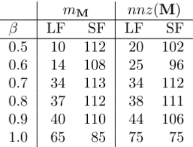
We investigate the tie-breaking mechanisms of QCC in order to choose the best strategy. For each β, we run the algorithm with the tie-breaking mechanism of favouring the nodes with smaller degrees first (SF) for expanding cliques and with the one favouring the nodes with larger degrees first (LF). We then counted how many times each mechanism was better (in the case of ties, the scores of both are incremented) with respect to the number mM of rows in M
and the number nnz(M) of nonzeros in M. The scores are shown in Table 1. As seen from this table, SF obtained a better score than LF in both metrics for all β in the test set. As β increases, the difference is less marked with often the same values for SF and LF. We see this because the scores add up to a number larger than the number of matrices, 119. For β = 0.5 there are only three such cases; this number increases with increasing β and is 31 for β = 1.0. From these experiments, we identify the tie-breaking mechanism of favouring the nodes with smaller degrees first as preferable, especially when β is small, as this yields fewer rows and nonzeros in M.
5.1.2 The parameter β in QCC.
The parameter β affects (i) the run time of the algorithm QCC; (ii) the number of rows of the approximate structural factor M (this also affects the number of nonzeros of M); (iii) the partitioning time (of the hypergraph partitioning
mM nnz(M) β LF SF LF SF 0.5 10 112 20 102 0.6 14 108 25 96 0.7 34 113 34 112 0.8 37 112 38 111 0.9 40 110 44 106 1.0 65 85 75 75
Table 1 – The number of matrices (each cell can be at most 119) in which a tie-breaking mechanism, smaller first (SF) or largest first (LF), was the best for differing β. time (s.) method nrows(M) nrows(A) nnz(M) nnz(A) StrDcp PaToH |L| |L|β=0.5 HQCC(0.5) 0.44 0.20 0.29 15.75 1.00 HQCC(0.6) 0.81 0.25 0.37 19.51 0.98 HQCC(0.7) 2.10 0.37 0.53 29.82 0.92 HQCC(0.8) 2.29 0.40 0.59 32.94 0.90 HQCC(0.9) 3.09 0.49 0.76 42.31 0.89 HQCC(1.0) 3.58 0.56 0.98 51.19 0.89 HCC 3.36 0.65 0.98 42.77 0.90 HM C37 2.01 0.47 0.69 27.76 0.88
Table 2 – Geometric mean over all matrices. The column StrDcp gives the geometric mean of the run time of different structural decomposition algorithms. The column |L|
|L|β=0.5 is the geometric mean of the fill-in with respect to that of β = 0.5.
tools applied to M); and (iv) the quality of the final ordering on the matrix A. It is expected that the smaller β is, the faster the QCC algorithm and the smaller the number of rows in the structural factor M, as there will be less quasi-cliques. The quality of the final ordering on the matrix A is expected to increase when increasing β, since the approximation becomes better. We now observe this expected outcome on the data set.
We present some statistics for all matrices in our data set for differing β in Table 2. In this table, we compare the effect of different structural decomposi-tion methods for creating hypergraphs. As seen in this table, the number of rows of M, i.e., the number of quasi-cliques, increases with increasing β (and also the number of nonzeros of M increases). Increasing β results in an improved ordering quality with HQCC(β). This however increases the run time for the
structural decomposition algorithm QCC and the run time for PaToH, where QCC is always much faster. The β values {0.5, 0.6, 0.7, 0.8, 0.9, 1.0} resulted in the most fill-in for 78, 23, 8, 0, 4, and 6 cases, respectively. Given these results, we identify 0.7 ≤ β ≤ 0.8 as a good choice: β values larger than 0.8 offer little improvement in the fill-in with increased run time for the partition-ing. For comparison, we also present results with HCC, using the clique cover
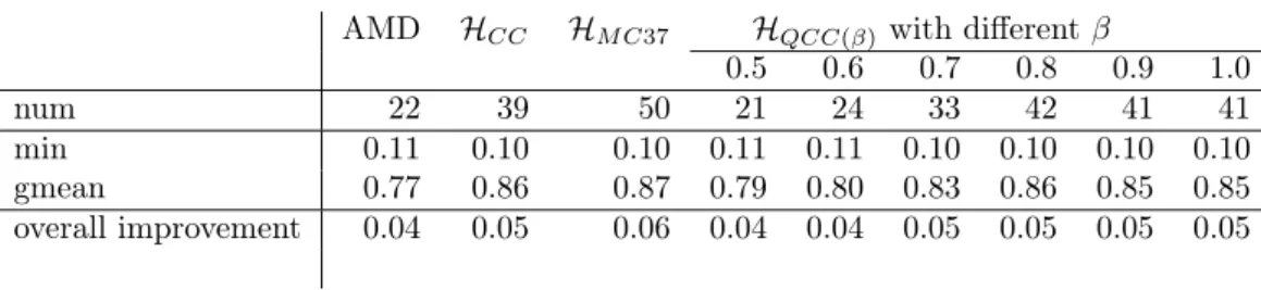
AMD HCC HM C37 HQCC(β)with different β 0.5 0.6 0.7 0.8 0.9 1.0 num 22 39 50 21 24 33 42 41 41 min 0.11 0.10 0.10 0.11 0.11 0.10 0.10 0.10 0.10 gmean 0.77 0.86 0.87 0.79 0.80 0.83 0.86 0.85 0.85 overall improvement 0.04 0.05 0.06 0.04 0.04 0.05 0.05 0.05 0.05 Table 3 – Performance of different algorithms with respect to MeTiS in terms of
fill-in for Cholesky factorization. The rows “num", “min", and “gmean" concern the cases where each method obtains strictly smaller fill-in than MeTiS. The last row shows the improvement in all 119 matrices where the method is used only in the matrices in which it was better than MeTiS, and MeTiS is used in the rest.
(CC) method [7], and also with the proposed HM C37. As seen from the results,
among the two exact structural decomposition methods, MC37 is preferable to CC. The sizes of the resulting hypergraphs are smaller for MC37 than when us-ing CC, and the resultus-ing fill-in is less when MC37 is used to obtain an orderus-ing. We defer further comparison of the structural decomposition methods in terms of fill-in to the next subsection.
5.1.3 Fill-in comparison with other methods.
The structural decomposition method should not be applied to all matrices for fill-reducing purposes. Consider, for example, the model problem which corresponds to the 5-point discretization of a 2D domain. In the corresponding graph, the maximum cliques are of size 2, and the best clique cover corresponds to the node-edge incidence matrix. This would create too many cliques. We prefer a small number of cliques or quasi-cliques (with respect to the number of vertices). Furthermore, if quasi-cliques are used, the pattern of MT
M should preferably be close to that of A. One way to use structural decomposition methods is to develop some criteria as to when to use them (and to use the state of the art methods, such as MeTiS, in the remaining cases). In preliminary investigations [17], we proposed such recipes for HCC, HQCC(0.8) and HM C37
where approximately a 2.5% improvement over MeTiS was obtained for each method. The “quality” setting of PaToH tries many algorithms in the multi-level framework to obtain improved results. This makes the quest for finding a recipe difficult. Therefore, our recipe for the use of a structural decomposition method is the ideal recipe: run MeTiS and the proposed method, and then choose the better result. Such ideal recipes are used in actual solvers [8, 15] as poly-algorithms.
Table 3 compares different methods with AMD and MeTiS. In this table, the number of matrices (among 119) in which a method obtained better fill-in than MeTiS is given in the row “num”. The minimum ratio and the geometric mean of fill-in with respect to that of MeTiS is given in the next two rows (for the matrices in which better results than those of MeTiS are obtained). By looking at the geometric means (the row gmean in the table), one notices
at least 13% improvement with respect to MeTiS with the proposed methods. However, this should be put into perspective by using all the matrices in the data set (this was our aim in choosing a large set of matrices automatically). To do so, we give the overall improvement over the whole data set in the final row of the table. The overall improvement of a method is computed by using the method when it gives a better result than MeTiS and by using MeTiS on other cases. For example, if HM C37 is used in 50 matrices from the data set
(where it obtains better results than MeTiS) and MeTiS is used in the other 69 matrices, we obtain an improvement of 6% with respect to using MeTiS only. As seen in the table, with a good choice of pattern factorization method, improvements of 4% to 6% in the fill-in are possible with respect to MeTiS. Also as seen in the table, the minimum ratio achieved by all methods with respect to MeTiS is around 0.10 (always on the matrix Sandia/ASIC_680k). Removing this matrix from the data set yields 2% overall improvement with HQCC(0.5),
3% overall improvement with AMD, HCC, HQCC(0.6), HQCC(0.7), HQCC(1.0),
and 4% overall improvement with HM C37, HQCC(0.8), and HQCC(0.9).
5.2
LU factorization
We used matrices satisfying the following properties. They are real, square, of order greater than 10000, have at least 4 nonzeros per row on average, have at most 20 million nonzeros and, as reported in the UFL collection, have a numer-ical symmetry smaller than 0.85. We exclude matrices recorded as “graph” in the UFL collection, because most of these matrices have nonzeros from a small set of integers (for example {−1, 1}) and are reducible. Again, these properties are used for automatically selecting a set of matrices from diverse application domains. There were a total of 41 matrices in the UFL collection satisfying these properties. On four of those matrices (with ids 898, 2260, 2265, and 2267) LU factorization took too much time with some of the ordering methods. We removed these matrices and experimented with 37 matrices in total. We first permuted the matrices columnwise with MC64 [13] to have the main diagonal corresponding to a maximum product matching and scaled the matrices such that the diagonal entries were one, and the others no larger than one in mag-nitude. We then added a diagonal shift (equal to the order of a matrix) to the matrices to ensure strong diagonal dominance. The matrices are then ordered with AMD [1] (run on A + AT), Colamd, Hund [25] (on A), and MeTiS (on
A + AT) and the resulting matrix was factorized with SuperLU [12, 33]. On any given matrix, the fill-in resulting from orderings returned by Colamd was always much worse than the others (this is expected as Colamd reduces a bound on the fill-in that could result from any row interchanges). This was also true for Hund for the same reason (the geometric mean of the ratio of the fill-in due to Hund to that due to MeTiS was 1.88 on the aforementioned data set). We therefore do not include the results with Colamd or with Hund and exclude these two ordering methods from the remaining discussion.
Given the success of HM C37 for the Cholesky factorization, we used MC37
on A + AT to get a structural factor as proposed in Section 3.2.3. This turned
out to be better than our bi-quasi-clique cover based heuristics. We therefore present results only with hypergraph partitioning based ordering where MC37 is used to obtain the hypergraphs. The overall algorithm is again denoted by HM C37.
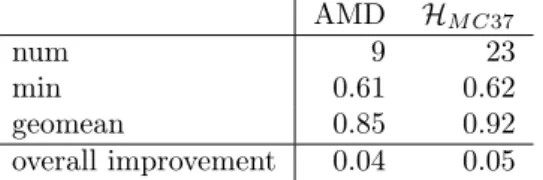
AMD HM C37
num 9 23
min 0.61 0.62
geomean 0.85 0.92
overall improvement 0.04 0.05
Table 4 – Performance of different algorithms with respect to MeTiS (with A+AT) in terms of fill-in for LU factorization on the matrices where the method obtains strictly less fill-in than MeTiS. The last row shows the improvement over all instances where the method is used only in the cases in which it was better than MeTiS and MeTiS is used in the rest. There are 37 matrices in total.
As was done in the previous subsection, we examine the potential of using the structural decomposition in Table 4. In this table, the number of cases in which a method has obtained better fill-in than MeTiS is given in the row “num”. The minimum ratio and the geometric mean of fill-in with respect to that of MeTiS is given in the next two rows. The final row gives the improvement over the whole data set, where a method is used when it gives a better result than MeTiS (that is, for example, HM C37is used in 23 matrices and MeTiS is used in
the other 14 matrices). As seen in the table, with a good choice of a structural decomposition method, an overall improvement of 4% to 5% in the ordering is possible. We note that if HM C37is used for all 37 matrices, the geometric mean
of the ratio to MeTiS is 0.98. In comparison, the geometric mean of the ratio of AMD to MeTiS is 1.16 if we include all 37 matrices.
5.3
QR factorization
We chose a set of 15 rectangular matrices (with ids 261, 799, 981, 1332, 1870, 1871, 1872, 1964, 2025, 2032, 2069, 2112, 2128, 2129, 2134) from the UFL col-lection. We added to the data set all nine matrices from the LPnetlib collection having more than 9000 rows and columns. On the LP matrices, earlier work by Çatalyürek et al. [7, Table 5.4] indicate that better results are to be expected. We have experimented within the context of Corollary 2. That is, we consider an M for a given A such that AT
A ≡ MTMholds.
When necessary, we transposed the matrices so that m ≥ n. We computed ATAand ordered the resulting matrix with MeTiS. In order to get a reasonable ordering and execution time when the matrices have dense rows or columns, we ordered only the non-dense rows/columns of ATA with MeTiS and appended
the dense rows to the end of the permutation (as done for AMD and variants). We sparsified the m×n input matrix A to obtain M (so that ATA ≡ MTM) and
applied PaToH to partition this matrix rowwise into K = max(2, bn/500c) parts. We then used an SBBD form as the constraint in Ccolamd [8, 10, 11] to find a column ordering for A. This approach is denoted by Hs. We also used MC37
on AT
A to obtain M, which is methodologically more comparable to MeTiS in requirements (both require the pattern of AT
A). This approach is denoted by HM C37. We used the Matlab function symbfact(A, ’col’, ’lower’) to
compute the number of nonzeros in R symbolically. Using symbfact and the Colamd results from the UFL collection (available in the data field amd_rnz),
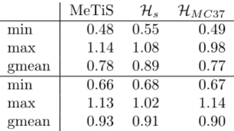
MeTiS Hs HM C37 min 0.48 0.55 0.49 max 1.14 1.08 0.98 gmean 0.78 0.89 0.77 min 0.66 0.68 0.67 max 1.13 1.02 1.14 gmean 0.93 0.91 0.90
Table 5 – Performance of different algorithms with respect to Colamd in terms of fill-in for QR factorization on general rectangular matrices (top half of the table) and on the LPnetlib matrices (in the bottom half of the table).
we compare Hsand HM C37with MeTiS below. Since on LP matrices we expect
a better result, we give results for the two different data sets separately so that we do not skew the results in favour of the proposed methods.
As seen from the top half of Table 5, MeTiS is 22% better than Colamd on general rectangular matrices. Using Hs and HM C37 in combination with
Ccolamdgreatly improves results. MeTiS is only 11% better than Hswhich can
be seen as Ccolamd with special constraints, and it is slightly worse than HM C37,
which can again be seen as Ccolamd with another set of constraints. The situ-ation improves for the LPnetlib matrices as expected in favour of Colamd, Hs
and HM C37. This time, MeTiS is better than Colamd by about 7%. Hypergraph
partitioning based methods Hs and HM C37are better than MeTiS by 2% and
3%, respectively.
The advantage of Colamd (with an SBBD form using Hs or without) with
respect to MeTiS and HM C37 is that the product ATA is not needed at all.
Even if there is no dense rows in A, the product is denser than A and forming and storing the product creates a non-negligible overhead.
We now briefly discuss what we gained by using sparsification to realize Corollary 1. Performing sparsification did not cause us to lose any quality (the geometric mean of the fill-in resulting from using the sparsified matrices to that resulting from using the original matrices was 1.01). The geometric mean of the ratio of the execution time of the hypergraph partitioning tool with the sparsified matrices to the original ones was 0.65. When the time spent in the sparsification routine was added before taking the ratios, the geometric mean became 0.68. Therefore, we conclude that with the sparsification method, we gain 32% in run time over the hypergraph partitioning tool without losing the quality of the resulting ordering.
5.4
Evaluation of the results
The tools for obtaining fill-reducing orderings for Cholesky factorization are well developed. In particular, local ordering methods (such as the approximate min-imum degree algorithm and its variants), and using graph partitioning based methods to set up constraints in the local ordering methods are well tested and improved over the years. Using hypergraph partitioning methods to obtain desirable forms to define the constraints is a recent approach, promising some advantages over the graph partitioning based method (discussed elsewhere [7,
Section 2.5]). Our methods were demonstrated to be better than the existing hypergraph partitioning based ordering methods. However, they are not con-sistently better than other existing methods. To us, it is very improbable to obtain consistently better results than the well established tools with a single method. Therefore, we think that it is necessary to try to combine all ap-proaches in a poly-algorithm to obtain the best results. With such an approach, we demonstrated improvements of about 5% and 6% in the Cholesky and LU factorization, indicating that the proposed approaches would be a very useful component in a poly-algorithm.
For QR factorization, the picture is much clearer. Using a hypergraph par-titioning method to obtain constraints for Ccolamd helps greatly. Using sparsi-fication helps to reduce run time for the hypergraph partitioning tool. The best identified hypergraph partitioning based ordering method obtains better results than MeTiS (while having the same inconvenience of forming and storing ATA
while building a structural factor using MC37). This seems to be avoidable by applying MC37’s algorithm on an implicitly stored matrix, instead of ATA.
On a special set of matrices, where a structural factorization already exists, the proposed method using MC37 and the simpler one, which does not form AT
A, obtain better results than MeTiS. These observations suggest the following: (i) the proposed hypergraph partitioning based ordering methods would again be very useful in a poly-algorithm; (ii) the hypergraph partitioning based ordering that does not need AT
Ais the method of choice (preferable to Colamd) when computing AT
Ais prohibitive.
6
Conclusion
We have discussed fill-reducing ordering methods for sparse Cholesky, LU, and QR factorization. Our approach is based on an (approximate) structural de-composition of the given input matrix, where the structural factor is expressed as a hypergraph. The proposed approach generalizes a previous study [7] in finding proper structural factors for Cholesky, and extends the results to the LU factorization. We have argued that for QR factorization, similar methods are applicable, where the overall scheme hinges on the fact that the R factor is the Cholesky factor of ATA.
In all three factorizations, we reported results that are better than MeTiS on some non-negligible number of matrices. Combining with MeTiS, the final averages are improved over 4% for Cholesky and LU factorization with respect to using MeTiS only. In QR factorization, one of the proposed methods based on the graph of AT
Aobtains results comparable to or better than MeTiS. In QR factorization of a class of matrices, where a structural decomposition already exists, the other proposed method, which never forms AT
A, obtains better results than MeTiS. In all three factorizations, a structural decomposition or sparsification of A are demonstrated to lead to a better quality ordering than one based on standard hypergraph partitioning approaches.
The structural decomposition of symmetric matrices with MC37 led to bet-ter results than most of the proposed structural decomposition methods. This was especially useful in the case of QR factorization. This encourages us to investigate adapting the algorithm to work on an implicitly stored ATA.
Acknowledgements
This work was partially supported by the LABEX MILYON (ANR-10-LABX-0070) of Université de Lyon, within the program “Investissements d’Avenir” (ANR-11-IDEX-0007) operated by the French National Research Agency (ANR), and also by ANR project SOLHAR (ANR-13-MONU-0007). The research of I. S. Duff was supported in part by the EPSRC Grant EP/I013067/1.
References
[1] P. R. Amestoy, T. A. Davis, and I. S. Duff. An approximate minimum degree ordering algorithm. SIAM Journal on Matrix Analysis and Appli-cations, 17(4):886–905, 1996.
[2] G. Ausiello, P. Crescenzi, V. Kann, Marchetti-Sp, G. Gambosi, and A. M. Spaccamela. Complexity and Approximation: Combinatorial Optimization Problems and Their Approximability Properties. Springer, 1999.
[3] C. Aykanat, A. Pinar, and Ü. V. Çatalyürek. Permuting sparse rectangular matrices into block-diagonal form. SIAM Journal on Scientific Computing, 25(6):1860–1879, 2004.
[4] I. Brainman and S. Toledo. Nested-dissection orderings for sparse LU with partial pivoting. SIAM Journal on Matrix Analysis and Applications, 23 (4):998–1012, 2002.
[5] Ü. V. Çatalyürek and C. Aykanat. Hypergraph-partitioning-based decom-position for parallel sparse-matrix vector multiplication. IEEE Transac-tions on Parallel and Distributed Systems, 10(7):673–693, Jul 1999. [6] Ü. V. Çatalyürek and C. Aykanat. PaToH: A Multilevel Hypergraph
Partitioning Tool, Version 3.0. Bilkent University, Department of Com-puter Engineering, Ankara, 06533 Turkey. PaToH is available at http: //bmi.osu.edu/~umit/software.htm„ 1999.
[7] Ü. V. Çatalyürek, C. Aykanat, and E. Kayaaslan. Hypergraph partitioning-based fill-reducing ordering for symmetric matrices. SIAM Journal on Sci-entific Computing, 33(4):1996–2023, 2011.
[8] Y. Chen, T. A. Davis, W. W. Hager, and S. Rajamanickam. Algo-rithm 887: CHOLMOD, supernodal sparse Cholesky factorization and up-date/downdate. ACM Trans. Math. Softw., 35(3):22:1–22:14, 2008. [9] T. A. Davis and Y. Hu. The University of Florida sparse matrix collection.
ACM Trans. Math. Softw., 38(1):1:1–1:25, 2011.
[10] T. A. Davis, J. R. Gilbert, S. I. Larimore, and E. G. Ng. A column approx-imate minimum degree ordering algorithm. ACM Transactions on Mathe-matical Software, 30(3):353–376, 2004.
[11] T. A. Davis, J. R. Gilbert, S. I. Larimore, and E. G. Ng. Algorithm 836: COLAMD, a column approximate minimum degree ordering algorithm. ACM Transactions on Mathematical Software, 30(3):377–380, Sept. 2004.
[12] J. W. Demmel, S. C. Eisenstat, J. R. Gilbert, X. S. Li, and J. W. H. Liu. A supernodal approach to sparse partial pivoting. SIAM Journal on Matrix Analysis and Applications, 20(3):720–755, 1999.
[13] I. S. Duff and J. Koster. On algorithms for permuting large entries to the diagonal of a sparse matrix. SIAM Journal on Matrix Analysis and Applications, 22:973–996, 2001.
[14] I. S. Duff and J. A. Scott. A parallel direct solver for large sparse highly unsymmetric linear systems. ACM Trans. Math. Softw., 30(2):95–117, June 2004. ISSN 0098-3500.
[15] I. S. Duff and J. A. Scott. Towards an automatic ordering for a symmetric sparse direct solvers. Technical Report RAL-TR-200601, Atlas Centre, Rutherford Appleton Laboratory (RAL), Oxon OX11 0QX, 2006.
[16] I. S. Duff and B. Uçar. Combinatorial problems in solving linear systems. In U. Naumann and O. Schenk, editors, Combinatorial Scientific Computing, chapter 2, pages 21–68. CRC Press, 2012.
[17] I. S. Duff, O. Kaya, E. Kayaaslan, and B. Uçar. Presentation at Workshop Celebrating 40 Years of Nested Dissection (ND40), available at http:// perso.ens-lyon.fr/bora.ucar/papers/nd40.pdf, July 2013.
[18] A. Ene, W. Horne, N. Milosavljevic, P. Rao, R. Schreiber, and R. E. Tar-jan. Fast exact and heuristic methods for role minimization problems. In Proceedings of the 13th ACM symposium on Access control models and technologies, SACMAT ’08, pages 1–10, New York, NY, USA, 2008. ACM. [19] J. M. Ennis, C. M. Fayle, and D. M. Ennis. Assignment-minimum clique
coverings. J. Exp. Algorithmics, 17:1.5:1.1–1.5:1.17, 2012.
[20] B. O. Fagginger Auer and R. H. Bisseling. A geometric approach to matrix ordering. CoRR, abs/1105.4490, 2011.
[21] A. George and M. T. Heath. Solution of sparse linear least squares problems using givens rotations. Linear Algebra and its Applications, 34(0):69–83, 1980.
[22] A. George and J. W. H. Liu. The evolution of the minimum degree ordering algorithm. SIAM Review, 31(1):1–19, 1989.
[23] A. George, M. Heath, and E. Ng. A comparison of some methods for solving sparse linear least-squares problems. SIAM Journal on Scientific and Statistical Computing, 4(2):177–187, 1983.
[24] G. H. Golub and C. F. Van Loan. Matrix Computations. The Johns Hopkins University Press, 3rd edition, 1996.
[25] L. Grigori, E. Boman, S. Donfack, and T. Davis. Hypergraph-based un-symmetric nested dissection ordering for sparse LU factorization. SIAM Journal on Scientific Computing, 32(6):3426–3446, 2010.
[26] HSL. HSL 2011: A collection of Fortran codes for large scale scientific computation, 2011. http://www.hsl.rl.ac.uk.
[27] Y. Hu and J. Scott. Ordering techniques for singly bordered block diagonal forms for unsymmetric parallel sparse direct solvers. Numerical Linear Algebra with Applications, 12(9):877–894, 2005.
[28] Y. F. Hu, K. C. F. Maguire, and R. J. Blake. A multilevel unsymmetric matrix ordering algorithm for parallel process simulation. Computers & Chemical Engineering, 23(11–12):1631–1647, 2000.
[29] G. Karypis and V. Kumar. MeTiS: A Software Package for Partitioning Unstructured Graphs, Partitioning Meshes, and Computing Fill-Reducing Orderings of Sparse Matrices Version 4.0. University of Minnesota, Depart-ment of Comp. Sci. and Eng., Army HPC Research Center, Minneapolis, 1998.
[30] O. Kaya, E. Kayaaslan, and B. Uçar. On the minimum edge cover and ver-tex partition by quasi-cliques problems. Technical report RR-8255, INRIA, Feb. 2013.
[31] T. Lengauer. Combinatorial Algorithms for Integrated Circuit Layout. Wiley–Teubner, Chichester, U.K., 1990.
[32] X. S. Li and J. W. Demmel. SuperLU_DIST: A scalable distributed-memory sparse direct solver for unsymmetric linear systems. ACM Trans. Math. Softw., 29:110–140, June 2003. ISSN 0098-3500.
[33] X. S. Li, J. W. Demmel, J. R. Gilbert, L. Grigori, M. Shao, and I. Yamazaki. SuperLU Users’ Guide. Technical Report LBNL-44289, Lawrence Berkeley National Laboratory, September 1999.
[34] J. Orlin. Contentment in graph theory: Covering graphs with cliques. Indagationes Mathematicae (Proceedings), 80(5):406–424, 1977.
[35] B. Uçar, Ü. V. Çatalyürek, and C. Aykanat. PaToH MATLAB interface. http://bmi.osu.edu/~umit/software.html„ July 2009.
[36] B. Uçar, Ü. V. Çatalyürek, and C. Aykanat. A matrix partitioning interface to PaToH in MATLAB. Parallel Computing, 36(5–6):254–272, 2010.