HAL Id: inria-00431469
https://hal.inria.fr/inria-00431469
Submitted on 20 Nov 2009
HAL is a multi-disciplinary open access
archive for the deposit and dissemination of
sci-entific research documents, whether they are
pub-lished or not. The documents may come from
teaching and research institutions in France or
abroad, or from public or private research centers.
L’archive ouverte pluridisciplinaire HAL, est
destinée au dépôt et à la diffusion de documents
scientifiques de niveau recherche, publiés ou non,
émanant des établissements d’enseignement et de
recherche français ou étrangers, des laboratoires
publics ou privés.
Upper Bounds on Stream I/O Using Semantic
Interpretations
Marco Gaboardi, Romain Péchoux
To cite this version:
Marco Gaboardi, Romain Péchoux. Upper Bounds on Stream I/O Using Semantic Interpretations.
23rd international Workshop on Computer Science Logic, CSL 2009, 18th Annual Conference of the
EACSL, Sep 2009, Coimbra, Portugal. pp.271-286, �10.1007/978-3-642-04027-6_21�. �inria-00431469�
Interpretations
Marco Gaboardi1 and Romain P´echoux2 1
Dipartimento di Informatica, Universit`a di Torino - [email protected]
2 Computer Science Department, Trinity College, Dublin - [email protected]
5
Abstract. This paper extends for the first time semantics interpretation tools to infinite data in order to ensure Input/Output upper bounds on first order Haskell like programs on streams. By I/O upper bounds, we mean temporal relations between the number of reads performed on the input stream elements and the number of output elements produced. We
10
study several I/O upper bounds properties that are of both theoretical and practical interests in order to avoid memory overflows.
1
Introduction
Interpretations are a well-established verification tool for proving properties of first order functional programs, term rewriting systems and imperative programs. 15
In the mid-seventies, Manna and Ness [1] and Lankford [2] introduced polyno-mial interpretations as a tool to prove the termination of term rewriting systems. The introduction of abstract interpretations [3], has strongly influenced the de-velopment of program verification and static analysis techniques. From their introduction, interpretations have been deeply studied up to now with hundred 20
of variations.
One variation of interest is the notion of quasi-interpretation [4]. It consists in a polynomial interpretation with relaxed constraints (large inequalities, functions over real numbers). Consequently, it no longer applies to termination problems (since well-foundedness is lost) but it allows to study program complexity in an 25
elegant way. Indeed, the quasi-interpretation of a first order functional program provides an upper bound on the size of the output values in the input size. The theory of quasi-interpretations has led by now to many theoretical develop-ments [4], for example, characterizations of the classes of functions computable in polynomial time and polynomial space. Moreover, the decidability of finding 30
a quasi-interpretation of a given program has been shown for some restricted class of polynomials [5, 6]. This suggests that quasi-interpretations can be inter-estingly exploited also in practical developments.
Quasi-interpretations have been generalized to sup-interpretations which are in-tensionnaly more powerful [7], i.e. sup-interpretations capture the complexity 35
of strictly more programs than quasi-interpretations do. This notion has led to a characterization of the NCk complexity classes [8] which is a complementary approach to characterizations using function algebra presented in [9].
A new theoretical issue is whether interpretations can be used in order to in-fer properties on programs computing over infinite data. Here we approach this 40
problem by considering Haskell programs over stream data. When considering stream data, size upper bounds have no real meaning. However, there are in-teresting I/O properties that are closely related to time. Indeed, we would like to be able to obtain relations between the input reads and the output writes of a given program, where a read (or write) corresponds to the computation of a 45
stream element in a function argument (resp. a stream element of the result). In this paper we study three criteria using interpretations in order to ensure three distinct kinds of I/O upper bounds on stream functions. The first crite-rion, named Length Based I/O Upper Bound (LBUB), ensures that the number of output writes (the output length) is bounded by some function in the number 50
of input reads. The second one, named Size Based I/O Upper Bound (SBUB), ensures that the number of output writes is bounded by some function in the input reads size. It extends the previous criterion to programs where the output writes not only depend on the input structure but also on its value. Finally, the last criterion, named Synchrony Upper Bound (SUB), ensures upper bounds 55
on the output writes size depending on the input reads size in a synchronous framework, i.e. when the stream functions write exactly one element for one read performed.
The above criteria are interesting from both a theoretical and a practical per-spective since the ensured upper bound properties correspond to synchrony and 60
asynchrony relations between program I/O.
Moreover, besides the particular criteria studied, this work shows that seman-tics interpretation can be fruitfully exploited in studying programs dealing with infinite data types. Furthermore, we carry out the treatment of stream proper-ties in a purely operational way. This shows that semantics interpretation are 65
suitable for the usual equational reasoning on functional programs. From these conclusions we aim our work to be a new methodology in the study of stream functional languages properties.
Related works The most studied property of streams is productivity, a notion dating back to [10]. Several techniques have been developed in order to ensure 70
productivity, e.g syntactical [10–12], data-flows analysis [13, 14], type-based [15– 18]. Some of these techniques can be adapted to prove different other properties, e.g. in [17], the authors gives different hint on how to use sized types to prove some kind of buffering properties. Unfortunately an extensive treatment using these techniques to prove other stream properties is lacking.
75
Outline of the paper In Section 2, we describe the considered first order stream language and its lazy semantic. In Section 3 we define the semantics interpretations and their basic properties. Then, in Section 4, we introduce the considered properties and criteria to ensure them. Finally in the last section we conclude by stating some questions on the use of interpretations for ensuring 80
2
Preliminaries
2.1 The sHask language
We consider a first order Haskell-like language, named sHask. Let X , C and F be disjoint sets denoting respectively the set of variables, the set of constructor 85
symbols and the set of function symbols. A sHask program is composed by a set of definitions described by the grammar in Table 1, where c ∈ C, x ∈ X , f ∈ F . We use the identifier t to denote a symbol in C ∪ F . Moreover the no-tation e, for some identifier e, is a short for the sequence e1, . . . , en. As usual,
application associates to the right, i.e. t e1 · · · encorresponds to the expression
90
((t e1) · · · ) en. In the sequel we will use the notation t −→e as a short for the
application t e1 · · · en.
The language sHask includes a Case operator to carry out pattern matching
p ::= x | c p1 · · · pn (Patterns)
e ::= x | t e1 · · · en| Case e of p1→ e1. . . pm→ em (Expressions)
v ::= c e1 · · · en (Values)
d ::= f x1 · · · xn = e (Definitions)
Table 1. sHask syntax
and first order function definitions. All the standard algebraic data types can be considered. Nevertheless, to be more concrete, in what follows we will consider 95
as example three standard data types: numerals, lists and pairs. Analogously to Haskell, we denote by 0 and infix + 1 the constructors for numerals, by nil and infix : the constructors for lists and by ( , ) the constructor for pairs.
Between the constant in C we distinguish a special error symbol ⊥ of arity 0 which corresponds to pattern matching failure. In particular, ⊥ is treated as the 100
other constructors, so for example we allow pattern matching on it. The set of Values contains the usual lazy values, i.e. expressions with a constructor as the outermost symbol.
In order to simplify our framework, we will put some syntactical restrictions on the shape of the considered programs. We restrict our study to outermost non 105
nested case definitions, this means that no Case appears in the e1, · · · , em of
a definition of the shape f(x) = Case e of p1→ e1, . . . , pm→ emand we
sup-pose that the function arguments and case arguments are the same, i.e. x = e. The goal of this restriction is to simplify the considered framework. We claim that it is not a severe restriction since every computable function can be easily 110
computed by a program using this convention.
Finally, we suppose that all the free variables contained in the expression eiof a
that patterns are non-overlapping. It entails that programs are confluent [19]. 115
Haskell Syntactic Sugar In the sequel we use the Haskell-like programming style. An expression of the shape f−→x = Case −→x of −→p1 → e1, . . . , −p→k → ek will
be written as a set of definitions f −→p1= e1, . . . , f−p→k = ek. Moreover, we adopt
the standard Haskell convention for the parenthesis, e.g. we use f (x + 1) 0 to denote ((f(x + 1))0).
120
2.2 sHask type system
Similarly to Haskell, we are interested only in well typed expressions. For sim-plicity, we consider only programs dealing with lists that do not contain other lists and we assure this property by a typing restriction similar to the one of [18]. Definition 1. The basic and value types are defined by the following grammar: 125
σ ::= α | Nat | σ × σ (basic types) A ::= a | σ | A × A | [σ] (value types)
where α is a basic type variable, a is a value type variable, Nat is a constant type representing natural numbers, × and [ ] are type constructors. The set of types contains elements of the shape A1→ (· · · → (An→ A)), for every n ≥ 0.
Notice that the above definition can be extended to standard algebraic data 130
types. In the sequel, we use σ, τ to denote basic types and A, B to denote value types. As in Haskell, we allow restricted polymorphism, i.e. a basic type variable α and a value type variable a represent every basic type and respectively every value type. As usual, → associates to the right, i.e. the notation A1 → · · · →
An→ A corresponds to the type A1→ (· · · → (An→ A)). Moreover, for notational
135
convenience, we will use −→A → B as an abbreviation for A1 → · · · → An → B
throughout the paper.
In what follows, we will be particularly interested in studying expressions of type [σ], for some σ, i.e. the type of finite and infinite lists over σ, in order to study stream properties. Well typed symbols, patterns and expressions are defined 140
using the type system in Figure 2. It is worth noting that the type system, in order to allow only first order function definitions, assigns types to constant and function symbols, but only value types to expressions.
As usual, we use :: to denote typing judgments, e.g. 0 :: Nat denotes the fact that 0 has type Nat. A well typed definition is a function definition where we 145
can assign the same value type A both to its left-hand and right-hand sides. As an aside, note that the symbol ⊥ can be typed with every value type A in order to get type preservation in the evaluation mechanism.
Stream terminology In this work, we are specifically interested in studying stream properties. Since both finite lists over σ and streams over σ can be typed 150
x :: A (Var) e :: A p1:: A · · · pm:: A e1:: A · · · em:: A Case e of p1→ e1. . . pm→ em:: A (Case) t :: A1→ · · · → An→ A (Tb) t :: A1→ · · · → An→ A e1:: A1 · · · en:: An t e1 · · · en:: A (Ts)
Table 2. sHask type system
with type [σ], we pay attention to particular classes of function working on [σ], for some σ. Following the terminology of [14], a function symbol f is called a stream function if it is a symbol of type f ::−[σ] → −→ →τ → [σ].
Example 1. Consider the following programs: merge :: [α] → [α] → [α × α]
merge (x : xs) (y : ys) = (x, y) : (merge xs ys)
nat :: Nat → [Nat] nat x = x : (nat (x + 1)) 155
merge and nat are two examples of stream functions
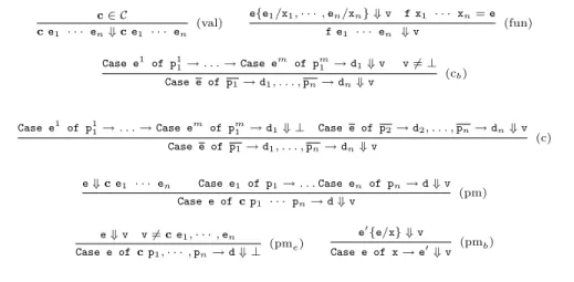
c ∈ C c e1 · · · en⇓ c e1 · · · en (val) e{e1/x1, · · · , en/xn} ⇓ v f x1 · · · xn= e f e1 · · · en ⇓ v (fun) Case e1 of p11→ . . . → Case em of pm1 → d1⇓ v v 6= ⊥ Case e of p1→ d1, . . . , pn→ dn⇓ v (cb)
Case e1 of p11→ . . . → Case em of pm1 → d1⇓ ⊥ Case e of p2→ d2, . . . , pn→ dn⇓ v
Case e of p1→ d1, . . . , pn→ dn⇓ v (c) e ⇓ c e1 · · · en Case e1 of p1→ . . . Case en of pn→ d ⇓ v Case e of c p1 · · · pn→ d ⇓ v (pm) e ⇓ v v 6= c e1, · · · , en Case e of c p1, · · · , pn→ d ⇓ ⊥ (pme) e 0{e/x} ⇓ v Case e of x → e0⇓ v (pmb)
Table 3. sHask lazy operational semantics
2.3 sHask lazy operational semantics
We define a lazy operational semantics for the sHask language. The lazy seman-tics we give is an adaptation of the one in [20] to our first order Haskell-like language, where we do not consider sharing for simplicity. The semantics is de-160
The computational domain is the set of Values. Values are particular expres-sions with a constructor symbol at the outermost position. Note that in par-ticular ⊥ is a value corresponding to pattern matching errors. As usual in lazy semantics, the evaluation does not explore the entire expression and stops once 165
the requested information is found.
The intended meaning of the notation e ⇓ v is that the expression e evaluates to the value v ∈ Values.
Example 2. Consider again the program defined in Example 1. It is easy to verify that: nat 0 ⇓ 0 : (nat (0 + 1)) and merge (nat 0) nil ⇓ ⊥.
170
2.4 Preliminary notions
We are interested in studying stream properties by operational finitary means, for this purpose, we introduce some useful programs and notions.
First, we define the usual Haskell take and indexing programs take and !! which return the first n elements of a list and the n-th element of a list, respectively. 175
As in Haskell, we use infix notation for !!. take :: Nat → [α] → [α]
take 0 s = nil
take (x + 1) nil = nil take (x + 1) (y : ys) = y : (take x ys)
!! :: [α] → Nat → α (x : xs) !! 0 = x (x : xs) !! (y + 1) = xs !! y
Second, we define a program eval that forces the (possibly diverging) full evalua-tion of expressions to fully evaluated values, i.e. values with no funcevalua-tion symbols. We define eval for every value type A as:
180
eval :: A → A
eval (c e1 · · · en) = ˆC (eval e1) · · · (eval em)
where ˆC is a program representing the strict version of the primitive construc-tor c. For example in the case where c is + 1 we can define ˆC as the program succ :: Nat → Nat defined by:
succ 0 = 0 + 1 succ (x + 1) = (x + 1) + 1 185
A set of fully evaluated values of particular interest is the set N = {n | n = ((· · · (0 + 1) · · · ) + 1)
| {z }
n times
and n :: Nat} of canonical numerals.
Then, we define a program lg that returns the number of elements in a finite partial list: lg :: [α] → Nat lg nil = 0 lg ⊥ = 0 lg (x : xs) = (lg xs) + 1 190
Example 3. In order to illustrate the behaviour of lg consider the expression ((succ 0) : (nil !! 0)). We have eval(lg ((succ 0) : (nil !! 0))) ⇓ 1.
Finally we introduce a notion of size for expressions:
Definition 2 (Size). The size of an expression e is defined as
|e| = 0 if e is a variable or a symbol of arity 0 |e| = X
i∈{1,...,n}
|ei| + 1 if e = t e1 · · · en, t ∈ C ∪ F .
Note that for each n ∈ N we have |n| = n. Throughout the paper, F (e) denotes the componentwise application of F to the sequence e, i.e. F (e1, · · · , en) =
195
F (e1), . . . , F (en). Moreover, given a sequence s = s1, · · · , sn, we will use the
notation |s| for |s1|, . . . , |sn|.
3
Interpretations
In this section, we introduce the interpretation terminology. The interpretations we consider are inspired by the notions of quasi-interpretation [4] and sup-200
interpretation [7] and are used as a main tool in order to ensure stream prop-erties. They basically consist in assignments over non negative real numbers following the terminology of [21]. Throughout the paper, ≥ and > denote the natural ordering on real numbers and its restriction.
Definition 3 (Assignment). An assignment of a symbol t ∈ F ∪ C of arity n is a functionLtM : (R+)n→ R+
. For each variable x ∈ X , we defineLxM = X , with X a fresh variable ranging over R+. This allows us to extend assignments L−M to expressions canonical ly. Given an expression t e1 . . . enwith m variables, its assignment is a function (R+)m
→ R+ defined by:
Lt e1 . . . enM = LtM(Le1M, · · · , LenM)
A program assignment is an assignmentL−M defined for each symbol of the pro-205
gram. An assignment is (weakly) monotonic if for any symbol t,LtM is an increas-ing (not necessarily strictly) function with respect to each variable, that is for every symbol t and all Xi, Yiof R+such that Xi≥ Yi, we haveLtM(. . . , Xi, . . .) ≥ LtM(. . . , Yi, . . .).
Notice that assignments are not defined on the Case construct since we only 210
apply assignments to expressions without Case.
Example 4. The functionL−M defined by LmergeM(U, V ) = U + V , L( , )M(U, V ) = U +V +1 andL:M(X, X S ) = X +X S +1 is a monotonic assignment of the program merge of example 1.
Now we define the notion of additive assignments which guarantees that the size 215
Definition 4 (Additive assignment). An assignment of a symbol c of arity n is additive if: LcM(X1, · · · , Xn) = Pn i=1Xi+ αc, with αc≥ 1 if n > 0, LcM = 0 otherwise.
The assignmentL−M of a program is cal led additive assignment if each construc-tor symbol of C has an additive assignment.
Definition 5 (Interpretation). A program admits an interpretation L−M if L−M is a monotonic assignment such that for each definition of the shape f
− →p = e 220
we have Lf−→pM ≥ LeM.
Notice that ifLtM is a subterm function, for every symbol t, then the considered interpretation is called a quasi-interpretation in the literature (used for inferring upper bounds on values). Moreover, ifLtM is a polynomial over natural numbers and the inequalities are strict then L−M is called a polynomial interpretation 225
(used for showing program termination).
Example 5. The assignment of example 4 is an additive interpretation of the program merge. Indeed, we have:
Lmerge (x : xs) (y : ys)M = LmergeM(Lx : xsM, Ly : ysM) By canonical extension =Lx : xsM + Ly : ysM By definition ofLmergeM =LxM + LxsM + LyM + LysM + 2 By definition ofL:M =L(x, y) : (merge xs ys)M Using the same reasoning Let → be the rewrite relation induced by giving an orientation from left to right to the definitions and let →∗ be its transitive and reflexive closure. We start by showing some properties on monotonic assignments.
Proposition 1. Given a program admitting the interpretationL−M, then for ev-230
ery closed expression e such that e →∗d, we have:LeM ≥ LdM
Proof. The proof is by induction on the derivation length [22]. ut Corollary 1. Given a program admitting the interpretationL−M, then for every closed expression e such that e ⇓ v, we have: LeM ≥ LvM
Proof. The lazy semantics is just a particular rewrite strategy. ut Corollary 2. Given a program admitting the interpretationL−M, then for every closed expression e such that eval e ⇓ v, we have:LeM ≥ LvM
235
Proof. By induction on the structure of expressions. ut It is important to relate the size of an expression and its interpretation. Lemma 1. Given a program having an interpretation L−M then there is a func-tion G : R+→ R+ such that for each expression e:
LeM ≤ G(|e|)
4
Bounded I/O properties and criteria
In this section, we define distinct stream properties related to time and space 240
and criteria using interpretations to ensure them. A naive approach would be to consider a time unit to be either a stream input read (the evaluation of a stream element in a function argument) or a stream output write (the evaluation of a stream element of the result). Since most of the interesting programs working on stream are non-terminating, this approach fails. In fact, we need a more concrete 245
notion of what time should be. Consequently, by time we mean relations between input reads and output writes, that is the ability of a program to return a certain amount of elements in the output stream (that is to perform some number of writes) when fed with some input stream elements.
4.1 Length based I/O upper bound (LBUB) 250
We focus on the relations that provide upper bounds on output writes. We here consider structural relations, that depend on the stream structure but not on the value of its elements. We point out an interesting property giving bounds on the number of generated outputs by a function in the length of the inputs. As already stressed, the complete evaluation of stream expressions does not terminates. So, 255
in order to deal with streams by finitary means, we ask, inspired by the well known Bird and Wadler Take Lemma [23], the property to hold on all the finite fragments of the streams that produce a result.
Definition 6. A stream function f :: −[σ] → −→ →τ → [σ] has a length based I/O upper bound if there is a function F : R+ → R+ such that for every expression
si:: [σi] and for every expression ei:: τi, we have that:
∀ ni∈ N, s.t. eval(lg(f (
−−−−−−→
take n s)−→e )) ⇓ m, F (max(|n|, |e|)) ≥ |m| where (−−−−−−→take n s) is a short for (take n1 s1) · · · (take nmsm).
Let us illustrate the length based I/O upper bound property by an example: 260
Example 6. The function merge of example 1 has a length based I/O upper bound. Indeed, consider F (X) = X, given two finite lists s, s0 of size n, n0 such that n ≤ n0, we know that eval(lg (merge s s0)) evaluates to an expression m such that m = n. Consequently, given two stream expressions e and e0such that eval(take n0 e0) ⇓ s0 and eval(take n e) ⇓ s, we have:
F (max(|n|, |n0|)) = F (max(n, n0)) = n0≥ n = |m|
4.2 A criterion for length based I/O upper bound
We here give a criterion ensuring that a given stream has a length based I/O upper bound. For simplicity, in the following sections, we suppose that the con-sidered programs do not use the programs lg and take.
Definition 7. A program is LBUB if it admits an interpretation L−M which 265
satisfiesL+1M(X ) = X + 1 and which is additive but on the constructor symbol : whereL:M is defined by L:M(X, Y ) = Y + 1.
We start by showing some basic properties of LBUB programs.
Lemma 2. Given a LBUB program, for every n :: Nat we haveLnM = |n|. Proof. By an easy induction on canonical numerals. ut Lemma 3. Given a LBUB program wrt the interpretation L−M, the interpreta-270
tion can be extended to the program lg by LlgM(X ) = X .
Proof. We check that the inequalities hold for every definition of lg. ut Lemma 4. Given a LBUB program wrt the interpretation L−M, the interpreta-tion can be extended to the program take byLtakeM(N , L) = N .
Proof. We check that the inequalities hold for every definition of take. ut Theorem 1. If a program is LBUB then each stream function has a length based I/O upper bound.
275
Proof. Given a LBUB program, if eval(lg (f (−take n s)−−−−−→ −→e )) ⇓ m then we know that Llg (f (−take n s)−−−−−→ −→e )M ≥ LmM, by Corollary 2. By Lemma 3, we obtain that Lf (−take n s)−−−−−→ −→eM ≥ LmM. By Lemma 4, we know that Lf (
−−−−−−→ take n s)−→eM = LfM(LnM LeM). Applying Lemma 2, we obtain |m| = LmM ≤ LfM(|n|, LeM). Finally, by Lemma 1, we know that there is a function G : R+ → R+ such that |m| ≤
LfM(|n|, G(|e|)). ut
Example 7. The merge program of example 1 admits the following additive inter-pretationLmergeM(X, Y ) = max(X, Y ), L( , )M(X, Y ) = X +Y +1 together with L: M(X, Y ) = Y + 1. Consequently, it is LBUB and, defining F (X ) = LmergeM(X, X ) we know that for any two finite lists s1 and s2 of length m1 and m2, we have
that if eval(lg(merge s1 s2)) ⇓ m then F (max(m1, m2)) ≥ |m| (i.e. we are able
280
to exhibit a precise upper bound).
4.3 Size based I/O upper bound (SBUB)
The previous criterion guarantees an interesting homogeneous property on stream data. However, a wide class of stream programs with bounded relations between input reads and output writes do not enjoy it. The reason is just that some 285
programs do not only take into account the structure of the input it reads, but also its value. We here point out a generalization of the LBUB property by considering an upper bound depending on the size of the stream expressions.
Example 8. Consider the following motivating example: append :: [α] → [α] → [α]
append (x : xs) ys = x : (append xs ys) append nil ys = ys
upto :: Nat → [Nat] upto 0 = nil
upto (x + 1) = (x + 1) : (upto x) 290
extendupto :: [Nat] → [Nat]
extendupto (x : xs) = append (upto x) (extendupto xs)
The program extendupto has no length based I/O upper bound because for each number n it reads, it performs n output writes (corresponding to a decreasing sequence from n to 1).
Now we introduce a new property dealing with size, that allows us to overcome 295
this problem.
Definition 8. A stream function f ::−[σ] → −→ →τ → [σ] has a size based I/O upper bound if there is a function F : R+
→ R+ such that, for every stream expression
si:: [σi] and for expression ei:: τi, we have that:
∀ ni∈ N, s.t. eval(lg(f (
−−−−−−→
take n s)−→e )) ⇓ m, F (max(|s|, |e|)) ≥ |m| where (−−−−−−→take n s) is a short for (take n1 s1) · · · (take nmsm).
Example 9. Since the program of example 8, performs n output writes for each number n it reads, it has a size based I/O upper bound.
Notice that this property informally generalizes the previous one, i.e. a size based 300
I/O upper bounded program is also length based I/O program, just because size always bounds the length. But the length based criterion is still relevant for two reasons, first it is uniform (input reads and output writes are treated in the same way), second it provides more accurate upper bounds.
4.4 A criterion for size based I/O upper bound. 305
We here give a criterion ensuring that a given stream has a size based I/O upper bound.
Definition 9. A program is SBUB if it admits an additive interpretation L−M such that L+1M(X ) = X + 1 and L:M(X, Y ) = X + Y + 1.
Lemma 5. Given a SBUB program wrt the interpretation L−M, the interpreta-310
tion can be extended to the program lg by LlgM(X ) = X .
Proof. We check that the inequalities hold for every definition of lg. ut Lemma 6. Given a SBUB program wrt the interpretation L−M, the interpreta-tion can be extended to the program take byLtakeM(N , L) = L.
Theorem 2. If a program is SBUB then each stream function has a size based I/O upper bound.
315
Proof. Given a SBUB program, then if eval(lg(f (−take n s)−−−−−→ −→e )) ⇓ m, for some stream function f, then Llg(f (
−−−−−−→
take n s) −→e )M ≥ LmM, by Corollary 2. By Lemma 5, we obtain thatLf (−take n s)−−−−−→ −→eM ≥ LmM. By Lemma 6, we know that Lf (
−−−−−−→
take n s)−→eM = LfM(LsM LeM). Applying Lemma 2 (which still holds because the interpretation of +1 remains unchanged), we obtain |m| =LmM ≤ LfM(LsM, LeM). Finally, by Lemma 1, we know that there is a function G : R+ → R+ such that
|m| ≤LfM(G(|s|), G(|e|)). ut
Example 10. The program extendupto of example 8 admits the following ad-ditive interpretation LnilM = L0M = 0, LappendM(X, Y ) = X + Y , LuptoM(X ) = LextenduptoM(X ) = 2 × X
2 together with
L+1M(X ) = X + 1 and L:M(X, Y ) = X + Y + 1. Consequently, it is SBUB and, defining F (X) = LextenduptoM(X ) we know that for any finite list s of size n, if eval(lg(extendupto s)) ⇓ m then 320
F (n) ≥ |m|, i.e. we are able to exhibit a precise upper bound. However notice that, as already mentioned, the bound is less tight than in previous criterion. The reason for that is just that size is an upper bound rougher than length. 4.5 Synchrony upper bound (SUB)
Sometimes we would like to be more precise about the computational complexity 325
of the program. In this case a suitable property would be synchrony, i.e. a finite part of the input let produce a finite part of the output. Clearly not every stream enjoys this property. Synchrony between stream Input and Output is a non-trivial question that we have already tackled in the previous subsections by providing some upper bounds on the length of finite output stream parts. In this 330
subsection, we consider the problem in a different way: we restrict ourselves to synchronous streams and we adapt the interpretation methodology in order to give upper bound on the output writes size with respect to input reads size. In the sequel it will be useful to have the following program:
lInd :: Nat → [α] → [α] lInd x xs = (xs !! x) : nil 335
We start to define the meaning of synchrony between input stream reads and output stream writes:
Definition 10. A stream function f :: −[σ] → −→ →τ → [σ] is said to be of type “Read, Write” if for every expression si:: σi, ei:: τi and for every n ∈ N:
If eval (lInd n (f→−s −→e )) ⇓ v and eval (f (lInd n s)−−−−−−→ −→e ) ⇓ v0 then v = v0 This definition provides a one to one correspondence between input stream reads and output stream writes, because the stream function needs one input read in order to generate one output write and conversely, we know that it will not 340
generate more than one output write (otherwise the two fully evaluated values cannot be matched).
Example 11. The following is an illustration of a “Read, Write” program: sadd :: [Nat] → [Nat] → [Nat]
sadd (x : xs) (y : ys) = (add x y) : (sadd xs ys) add :: Nat → Nat → Nat
add (x + 1) (y + 1) = ((add x y) + 1) + 1 add (x + 1) 0 = x + 1 add 0 (y + 1) = y + 1 345
In this case, we would like to say that for each integer n, the size of the n-th output stream element is equal to the sum of the two n-th input stream elements. Definition 11. A “Read, Write” stream function f :: −[σ] → −→ →τ → [σ] has a synchrony upper bound if there is a function F : R+→ R+ such that for every
expression si:: [σi], ei:: τi and for every n ∈ N:
If eval(si !! n) ⇓ wi and eval((f−→s −→e ) !! n) ⇓ v then F (max(|w|, |e|)) ≥ |v|
Another possibility would have been to consider n to m correspondence between inputs and outputs. However such correspondences can be studied with slight changes over the one-one correspondence.
350
4.6 A criterion for synchrony upper bound
We begin to put some syntactical restriction on the considered programs so that each stream function symbol is “Read, Write” with respect to this restriction. Definition 12. A stream function f :: −[σ] → −→ →τ → [σ] is synchronously re-stricted if it can be written (and maybe extended) by definitions of the shape:
f (x1: xs1) · · · (xn: xsn) −→p = hd : (f xs1· · · xsn −→e )
f nil · · · nil −→p = nil where xs1, . . . , xsn do not appear in the expression hd.
Now we may show the following lemma. 355
Lemma 7. Every synchronously restricted function is “Read, Write”.
Proof. By induction on numerals. ut Definition 13. A program is SUB if it is synchronously restricted and admits an additive interpretationL−M but on : where L:M is defined by L:M(X, Y ) = X . Fully evaluated values, i.e. values v containing only constructor symbols, have the following remarkable property.
360
Lemma 8. Given an additive assignmentL−M, for each ful ly evaluated value v: |v| ≤LvM.
Proof. By structural induction on fully evaluated values. ut Theorem 3. If a program is SUB then each stream function admits a synchrony upper bound.
Proof. By Lemma 7, we can restrict our attention to a “Read, Write” stream function f ::−[σ] → −→ →τ → [σ] s.t. ∀n ∈ N, we both have eval ((f−→s −→e ) !! n) ⇓ v and eval(si !! n) ⇓ wi.
We firstly prove that eval (f −−−−−→(w : nil) −→e ) ⇓ v : nil. By assumption, we have eval((f−→s −→e ) !! n) ⇓ v, so in particular we also have eval (((f −→s −→e ) !! n) : nil) ⇓ v : nil. By definition of “Read, Write” function, eval ((f ((−→s !! n) : nil) −→e ) ⇓ v : nil and since by assumption eval(si !! n) ⇓ wi we can conclude
eval (f−−−−−→(w : nil) −→e ) ⇓ v : nil.
By Corollary 2, we have Lf −−−−−→(w : nil) −→eM ≥ Lv : nilM. By definition of SUB programs, we know thatL:M(X, Y ) = X and, consequently, LfM(Lw : nilM, LeM) = LfM(LwM, LeM) ≥ Lv : nilM = LvM. By Lemma 8, we have LfM(LwM, LeM) ≥ |v|. Finally, by Lemma 1, there exists a function G : R+
→ R+such that
LfM(G(|w|), G(|e|)) ≥ |v|. We conclude by taking F (X) =LfM(G(X ), G(X )). ut Example 12. The program of example 11 is synchronously restricted (it can be 365
extended in such a way) and admits the following additive interpretationL0M = 0, L+1M(X ) = X + 1, LaddM(X, Y ) = X + Y , LsaddM(X, Y ) = X + Y and L:M(X, Y ) = X. Consequently, the program is SUB and admits a synchrony upper bound. Moreover, taking F (X) = LsaddM(X, X ), we know that if the k-th input reads evaluate to numbers n and m then F (max(|m|, |n|)) is an upper bound on the k-th 370
output size.
5
Conclusion
In this paper, we have applied interpretation methods for the first time to a lazy functional stream language, obtaining several criteria for bounds on the input read and output write elements. This shows that interpretations are a valid tool 375
to well ensure stream functions properties. Many interesting properties should be investigate, in particular memory leaks and overflows [17, 18]. These questions are strongly related to the notions we have tackled in this paper. For example, consider the following program :
odd :: [α] → [α]
odd (x : y : xs) = x : (odd xs)
memleak :: [α] → [α × α] memleak s = merge (odd s) s 380
The evaluation of an expression memleak s leads to a memory leak. Indeed, merge reads one stream element on each of its arguments in order to output one element and odd needs to read two stream input elements of s in order to output one element whereas s just makes one output for one input read. Consequently, there is a factor 2 of asynchrony between the two computations on s. Which 385
s) in order to compute the n-th output element. From a memory management perspective, it means that all the elements between sn and s2×n have to be
stored, leading the memory to a leak. We think interpretations could help the programmer to prevent such ”bad properties” of programs.
390
References
1. Manna, Z., Ness, S.: On the termination of Markov algorithms. In: Third hawaii international conference on system science. (1970) 789–792
2. Lankford, D.: On proving term rewriting systems are noetherien. tech. rep. (1979) 3. Cousot, P., Cousot, R.: Abstract interpretation: a unified lattice model for static
395
analysis of programs by construction or approximation of fixpoints. Proceedings of ACM POPL’77 (1977) 238–252
4. Bonfante, G., Marion, J.Y., Moyen, J.Y.: Quasi-interpretations, a way to control resources. TCS - Accepted.
5. Amadio, R.: Synthesis of max-plus quasi-interpretations. Fundamenta
Informati-400
cae, 65(1–2), 2005.
6. Bonfante, G., Marion, J.Y., Moyen, J.Y., P´echoux, R.: Synthesis of quasi-interpretations. LCC2005, LICS Workshop (2005) http://hal.inria.fr/. 7. Marion, J.Y., P´echoux, R.: Sup-interpretations, a semantic method for static
anal-ysis of program resources. ACM TOCL 2009, Accepted. http://tocl.acm.org/.
405
8. Marion, J.Y., P´echoux, R.: A Characterization of NCk by First Order Functional Programs. LNCS 4978 (2008) 136
9. Bonfante, G., Kahle, R., Marion, J.Y., Oitavem, I.: Recursion schemata for NC k. LNCS 5213 (2008) 49–63
10. Dijkstra, E.W.: On the productivity of recursive definitions. EWD749 (1980)
410
11. Sijtsma, B.: On the productivity of recursive list definitions. ACM TOPLAS 11(4) (1989) 633–649
12. Coquand, T.: Infinite objects in type theory. LNCS 806 (1994) 62–78
13. Wadge, W.: An extensional treatment of dataflow deadlock. TCS 13 (1981) 3–15 14. Endrullis, J., Grabmayer, C., Hendriks, D., Isihara, A., Klop, J.: Productivity of
415
Stream Definitions. LNCS 4639 (2007) 274
15. Telford, A., Turner, D.: Ensuring streams flow. LNCS 1349 (1997) 509–523 16. Buchholz, W.: A term calculus for (co-) recursive definitions on streamlike data
structures. Annals of Pure and Applied Logic 136(1-2) (2005) 75–90
17. Hughes, J., Pareto, L., Sabry, A.: Proving the correctness of reactive systems using
420
sized types. Proceedings of ACM POPL’96 (1996) 410–423
18. Frankau, S., Mycroft, A.: Stream processing hardware from functional language specifications. Proceeding of IEEE HICSS-36 (2003)
19. Huet, G.: Confluent reductions: Abstract properties and applications to term rewriting systems. Journal of the ACM 27(4) (1980) 797–821
425
20. Launchbury, J.: A natural semantics for lazy evaluation. Proceedings of POPL’93 (1993) 144–154
21. Dershowitz, N.: Orderings for term-rewriting systems. TCS 17(3) (1982) 279–301 22. Marion, J.Y., P´echoux, R.: Characterizations of polynomial complexity classes
with a better intensionality. Proceedings ACM PPDP’08 (2008) 79–88
430
23. Bird, R., Wadler, P.: Introduction to Functional Programming. Prentice Hall (1988)
A
Proofs
Proof of Corollary 2 If e ⇓ c −→e then eval e ⇓ c −→v , for some vi such
that eval ei ⇓ vi. By Corollary 1 LeM ≥ Lc − →
eM and by induction hypothesis LeiM ≥ LviM, so by monotonicity of LcM we have LeM ≥ Lc
− → eM ≥ Lc − → vM.
Proof of Lemma 1 Define F (X) = max(maxt∈C∪FLtM(X, . . . , X ), X ). Notice that F is subterm. If e is a constant then LeM ≤ F (|e|) because e ∈ C ∪ F and F (X) ≥ LeM. Suppose, by induction hypothesis, that for every expression di of size strictly smaller than n we haveLdiM ≤ F
|di|(|d
i|), where Fn+1(X) =
F (Fn(X)) and F0(X) = X, and consider an expression e = t−→d of size n.
LeM = LtM(L − → dM) ≤LtM(F|d1|(|d 1|), . . . , F|dn|(|dn|)) By I.H. ≤LtM(F|dj|(|d j|), . . . , F|dj|(|dj|)) By monotonicity if |dj| = max i∈{1,n}|di | ≤ F (F|dj|)(|d j|) By definition of F ≤ F|dj|+1(|e|) By monotonicity of F ≤ F|e|(|e|) By subterm property of F
Just take G(X) = FX(X).
Proof of Lemma 2 By induction on numerals, |0| = L0M = 0, by additivity ofL−M. Suppose it holds for n and consider n + 1. We have Ln + 1M = L+1M(LnM) = LnM + 1 = |n| + 1 = |n + 1|, by induction hypothesis and since L+1M(X ) = X + 1.
Proof of Lemma 3 We check that the inequalities hold for every definition of the symbol lg:
Llg nilM = LlgM(LnilM) = LnilM = 0 = L0M (By additivity) Llg ⊥M = LlgM(L⊥M) = L⊥M = 0 = L0M (By additivity) Llg (x : xs)M = Lx : xsM = LxsM + 1 = Llg xs + 1M (By definition ofL+1M)
Proof of Lemma 4 SinceL+1M(X ) = X + 1, we check that the inequalities hold for every definition of the symbol take:
Ltake 0 sM = LtakeM(L0M, LsM) = L0M = 0 = LnilM (By additivity) Ltake (x + 1) nilM = X + 1 ≥ 0 = LnilM (By additivity) Ltake (x + 1) (y : ys)M = X + 1 = Ly : (take x ys)M
Proof of Lemma 5 We check that the inequalities hold for every definition of the symbol lg:
Llg nilM = LlgM(LnilM) = LnilM = 0 = L0M (By additivity) Llg ⊥M = LlgM(L⊥M) = L⊥M = 0 = L0M (By additivity) Llg (x : xs)M = Lx : xsM = LxM + LxsM + 1 ≥ Llg xs + 1M (Definition ofL+1M) Proof of Lemma 6 SinceL:M(X, Y ) = X + Y + 1, we check that the inequalities hold for every definition of the symbol take:
Ltake 0 sM = LtakeM(L0M, LsM) = LsM ≥ 0 = LnilM (∀s, LsM ∈ R
+)
Ltake (x + 1) nilM = LnilM = 0 = LnilM (By additivity) Ltake (x + 1) (y : ys)M = LyM + LysM + 1 = Ly : (take x ys)M
Proof of Lemma 7 Consider a synchronously restricted function f :: −[σ] →→ −
→τ → [σ] such that for every n ∈ N, both eval (lInd n (f −→s −→e )) ⇓ v and eval (f (−lInd n s)−−−−−→ −→e ) ⇓ v0. We prove by induction on n that v = v0.
Consider the case n = 0. By hypothesis eval (lInd 0 (f −→s −→e )) ⇓ v, so eval (((f−→s −→e )!!0) : nil) ⇓ v1: nil with v = v1: nil. Since f is synchronously
restricted we have both si⇓ hdi: taili and (f
−−−−−−→
hd : tail−→e ) ⇓ hd : tail More-over, hd does not contains taili and is such that eval hd ⇓ v1.
Now, by assumption we also have eval (f (−lInd 0 s)−−−−−→ −→e ) ⇓ v0. Since si ⇓ hdi :
taili, in particular lInd 0 si⇓ hdi: nil. So, since f is synchronously restricted
we also have f (−−−−−→hd : nil)−→e ⇓ hd : (f−nil−→−→e ). Now since eval hd ⇓ v1and since
eval (f−nil−→−→e ) ⇓ nil we can conclude v0= v1: nil = v.
Consider the case n = m + 1. By hypothesis eval (lInd (m + 1) (f −→s −→e )) ⇓ v, so eval (((f −→s −→e ) !! (m + 1)) : nil) ⇓ v1 : nil with v = v1 : nil. In
par-ticular (f −→s −→e ) ⇓ hd : tail and eval ((tail !! m) : nil) ⇓ v1 : nil. Since
f is synchronously restricted, si ⇓ hdi : taili, hd does not contains taili
and tail = f −−→tail −→e . So, eval (((f −−→tail −→e ) !! m) : nil) ⇓ v1 : nil that
means eval (lInd m (f−−→tail −→e )) ⇓ v1 : nil. By induction hypothesis we have
eval (f (−−−−−−−−→lInd m tail)−→e )) ⇓ v1: nil.
Now, consider eval (f (−−−−−−−−−−→lInd (m + 1) s) −→e )) ⇓ v0. Clearly lInd (m + 1) si ⇓
(si !! (m + 1)) : nil and since si ⇓ hdi : taili, in particular eval ((si !! (m +
1)) : nil) ⇓ vi if and only if eval ((taili !! m) : nil) ⇓ vi. So, we have
eval (f (−−−−−−−−→lInd m tail)−→e )) ⇓ v0 and from this follows v = v0.
Proof of Lemma 8 We show the result by structural induction on fully eval-uated values. For a constant, we have |c| =LcM = 0, by additivity. Now suppose that |vi| ≤LviM and take a fully evaluated value of the shape c v1. . . vn. Then:
|c v1. . . vn| = X i∈{1,...,n} |vi| + 1 ≤ X i∈{1,...,n} LviM + αc=Lc v1. . . vnM
The inequality is a consequence of the combination of inductive hypothesis and the fact that, by definition of additive assignments, there is a constant αc ≥ 1
435